


 DownLoad:


-
Landfalling tropical cyclones (TCs) cause hazardous disasters, such as strong winds, heavy rainfall, and storm surge, in China (Xu et al., 2015). During 1983–2006, landfalling TCs on average led to an annual economic loss of 28.7 billion RMB and an annual loss of life of 472 in China (Zhang et al., 2009). The TC-induced disasters are closely associated with the TC intensity and structure (Chen et al., 2013). However, the forecasts of TC intensity and structure have shown slow improvement and are still challenging (Elsberry et al., 2013; DeMaria et al., 2014). Thus, to reduce losses caused by landfalling TCs in China, it is essential to improve TC forecasting, especially in terms of intensity, strong winds, and heavy rainfall (Duan et al., 2019).
Due to inaccurate initial conditions, imperfect model formulations (e.g., physical parameterizations), and chaotic natures of TCs, there are inevitable uncertainties in TC forecasting. Thus, ensemble forecasts that can sample such forecast uncertainties are preferred (Emanuel, 2018; Palmer, 2019). In the past two decades, the application of ensemble forecasting has produced encouraging improvements in TC forecasting for both track (Rappaport et al., 2009; Yamaguchi et al., 2009) and intensity (Yu et al., 2013; Zhang et al., 2014c).
Recently, the development of high-resolution ensembles for TC forecasting has become increasingly important (Hamill et al., 2012; Gall et al., 2013), because increasing the horizontal resolution of numerical weather prediction (NWP) models has shown improvements in TC intensity prediction and structural realism (Davis et al., 2010; Goldenberg et al., 2015). For the global ensemble of the European Centre for Medium-range Forecasts (ECMWF), increasing the horizontal resolution from 18 km to 5 km was confirmed by Magnusson et al. (2019) to improve the forecasts of hurricane Irma (2017) for both track and intensity. A mesoscale ensemble prediction system (namely TREPS; Zhang, 2018a, Z18 hereafter) with a resolution of approximately 9 km was recently constructed based on the tropical regional atmosphere model for the South China Sea (CMA-TRAMS), which is an NWP model developed from the framework of the Global/Regional Assimilation and Prediction System (GRAPES; Chen et al., 2008). Compared with the ECMWF ensemble, TREPS generally improved TC forecasting for intensity, strong winds, and heavy rainfall for 19 TCs making landfall in China during 2014–16 (Z18).
It is important to consider uncertainties of sea surface temperature (SST) in ensembles for TC forecasting, given the significant impact of SST on TC formulation and evolution (e.g., Emanuel, 1986; Zhang et al., 2014b). Kunii and Miyoshi (2012) improved the track forecasting for both typhoons Sinlaku (2008) and Jangmi (2008) by adding SST perturbations in a regional ensemble, which were generated by randomly choosing SST analyses from climatology. Such a perturbation strategy for SST allows for some spatial correlations in SST uncertainties that are consistent with climatology and showed benefits in ensemble forecasting of TC intensity (Torn, 2016). For TREPS, SST perturbations were generated by adding spatially uncorrelated white noise and showed positive impacts for forecasts of most of the TC cases [e.g., typhoon Mujigae (2015)] examined in Z18. However, some TC cases [e.g., typhoon Soudelor (2015)] did degrade in the forecast performance due to SST perturbations in TREPS (Z18). Thus, it is necessary to explore how to optimally perturb SST in reginal ensembles (especially TREPS) to improve TC forecasting.
The representation of uncertainties in physical parameterizations in ensembles has received greater attention (Christensen et al., 2015; Leutbecher et al., 2017). Due to the advantages in generating statistically consistent ensemble distributions (Berner et al., 2009; Sanchez et al., 2016), the approach of stochastically perturbing physical parameterizations has gained wide acceptance in recent years to create perturbed model physics.
One of the stochastic perturbation approaches is the Stochastically Perturbed Parameterization Tendency (SPPT; Palmer et al., 2009; Berner et al., 2015), which is used to sample the distribution of the subgrid physics tendencies. SPPT has been recently implemented in high-resolution regional ensembles and shown benefits in predicting some surface variables especially in terms of reliability (Bouttier et al., 2012; Romine et al., 2014). However, one of the drawbacks of the traditional SPPT scheme is that the same level of uncertainty is assigned to all processes and all atmospheric situations (Leutbecher et al., 2017). To address such a drawback, “independent SPPT”, where the uncertainty in tendency of each parametrization scheme is represented independently from the others, was proposed by Christensen et al. (2017). Recently, the independent physical parameterization-based SPPT (ipSPPT) approach, where the partial tendencies of the physical parametrizations are sequentially perturbed with individual stochastic patterns, was proposed by Wastl et al. (2019a) and confirmed to be effective in improving probabilistic forecasts of surface variables in a high-resolution ensemble. While there are increasing studies highlighting the benefits of the SPPT scheme and its variants in high-resolution regional ensembles especially for surface variables, fewer studies have investigated the impacts of SPPT on TC forecasting. For the Taiwan mesoscale ensemble, adding SPPT showed little impact on the track forecasting of typhoon Goni (2015) (Li et al., 2020). For TREPS, although adding SPPT improved both TC track and intensity forecasting for typhoons Soudelor (2015) and Mujigae (2015), SPPT showed less contribution to forecast perturbations than the multi-physics scheme (Z18). Melhauser et al. (2017) evaluated the impacts of SPPT on the convection-permitting ensemble forecasting of hurricanes Sandy (2012) and Edouard (2014) and found mixed and negative impacts on track and intensity forecasting, respectively. Thus, it is still unclear how to use or improve SPPT to improve TC forecasting.
To represent model physics uncertainties directly at the process level, the Stochastically Perturbed Parameterization (SPP; Jankov et al., 2017; Ollinaho et al., 2017) was proposed to stochastically perturb poorly constrained parameters in the physical parameterizations. SPP has gained increasing acceptance in high-resolution regional ensembles and already shown some advantages in predicting surface variables (Baker al., 2014; McCabe et al., 2016; Jankov et al., 2019; Wang et al., 2020). Recently, a combination of SPP and SPPT has been recommended to more comprehensively represent model uncertainties in both global (Ollinaho et al., 2017; Leutbecher et al., 2017) and regional (Jankov et al., 2017) ensembles. Such a combination has shown benefits in predicting some low-level variables in regional ensembles (Jankov et al., 2017, 2019; Wang et al., 2019; Wastl et al., 2019b; Xu et al., 2020). Despite the increasing prevalence of SPP in ensembles, less attention has been given to the benefits of SPP in TC forecasting. Torn (2016) found that adding stochastic perturbations in the exchange coefficients has limited impacts on TC intensity variability and leads to mixed impacts on TC intensity forecasting. Therefore, developing SPP to improve TC forecasting is still a work in progress.
Although TREPS has shown some encouraging performance in predicting landfalling TCs, the current version of TREPS is still deficient in generating perturbations for both surface and model physics. Thus, further improving TREPS is essential to better meet the requirements of operational refined weather services for TC forecasting, especially in terms of intensity, strong winds, and heavy rainfall. The goal of this paper is to investigate the impacts of new implementing strategies for surface and model physics perturbations in TREPS on the forecasts of landfalling TCs, which are characterized by different intensity changes. To achieve this goal, ensemble forecasts based on TREPS with a modified SST-perturbation strategy, a modified SPPT scheme, and a combination of SPPT and SPP are conducted, respectively, and compared with ensemble forecasts of TREPS carried out in Z18. The TREPS configuration and experimental design are described in section 2. Section 3 provides an overview of the 19 TCs studied here, along with the case classification. Results of the experiments are presented in sections 4. Section 5 concludes the paper and provides further discussion.
-
TREPS is constructed based on TRAMS (Chen et al., 2014), which is a non-hydrostatic regional model using a semi-implicit, semi-Lagrangian scheme for time integration. TRAMS adopts a horizontal grid designed on a longitude–latitude mesh with Arakawa C-grid staggering and includes 385 × 305 horizontal grid points with the horizontal resolution of 0.09° × 0.09°. The center of TRAMS domain is determined according to the position of the TC center, which is reported in the official real-time warning information from the China Meteorological Administration (CMA). The vertical coordinate is terrain following with Charney–Philips vertical layer skipping (Charney and Phillips, 1953), and there are 55 vertical layers. The WRF Single-Moment 6-class (WSM6) microphysics (Hong et al., 2004) and Monin–Obukhov (Beljaars, 1995) surface layer parameterization schemes are used. A detailed description of the forecast model of TREPS is given in Z18.
TREPS is initiated when a TC approaches the Chinese mainland and is suspended when the TC has made landfall. There are 30 perturbed ensemble members in TREPS, each of which issues 60-h forecasts twice per day at 0000/1200 UTC. The deterministic or unperturbed member of TREPS is cold started, with the analyses and forecasts from the 0.125° × 0.125° ECMWF high-resolution forecasts used as the initial condition and lateral boundary conditions (LBCs), respectively. The perturbed members are generated by adding perturbations to the initial condition, LBCs, surface, and model physics of the unperturbed member.
-
The baseline configuration of TREPS in perturbation generation is briefly provided below and the interested reader is referred to Z18 for additional details and justification for the choices made in designing perturbations. In particular, Z18 (see Fig. 2 therein) illustrated how to determine some key parameters [e.g., the standard deviation (δ), perturbation range (γ), amplitude range (λ), spatial decorrelation scale (κ), and temporal decorrelation scale (τ) introduced below] used in the generation of perturbations (especially for SST and SPPT) in a detailed way.
The downscaling perturbations are derived from the first 30 perturbed ensemble members of the 0.5° × 0.5° ECMWF ensemble forecasts (Buizza, 2014). The initial perturbations are the linear combination of downscaling perturbations and balanced random perturbations (Barker, 2005), which are generated by taking Gaussian random draws with zero mean and covariances used in the GRAPES three-dimensional variational (3D-Var) system (Xue et al., 2008). Downscaling perturbations are also added to LBCs of the unperturbed member with the interval of 6 h.
SST perturbations are implemented by adding Gaussian random numbers with the mean of 0 and standard deviation of δ to the surface temperature of the unperturbed member. Such perturbations are not implemented when the distance between the grid point and TC center reported in the real-time warning information valid at the initial time is greater than the length γ. The implementation of SST perturbations includes three additional steps: 1) perturbations are multiplied by a factor that increases linearly from 0 at distance γ to 1 at the wind radius of 17.2 m s−1 reported in the real-time warning information; 2) the amplitude of perturbations is restricted within the range of ±λδ to avoid excessive perturbations; and 3) perturbations are kept unchanged during the entire model integration.
The multi-physics scheme (Houtekamer et al., 1996; Stensrud et al., 2000; Hacker et al., 2011b) is combined with SPPT to generate model physics perturbations. In multi-physics, four combinations of physics packages for parameterizing the cumulus convection and planetary boundary layer (PBL) processes are constructed based on the Kain-Fritsch (KF; Kain and Fritsch, 1990; Kain, 2004) and the simplified Arakawa-Schubert (SAS; Pan and Wu, 1995; Han and Pan, 2006) schemes, and the medium-range forecast (MRF; Hong and Pan, 1996) and the Yonsei University (YSU; Hong et al., 2006) PBL schemes. Eight, eight, seven, and seven perturbed ensemble members are selected randomly to use the SAS/MRF, SAS/YSU, KF/MRF, and KF/YSU schemes, respectively. In SPPT, a random field r drawn from a Gaussian distribution with mean of zero, standard deviation of 0.5, spatial decorrelation scale of κ, and temporal decorrelation scale of τ is generated. To avoid unrealistic perturbations causing numerical instability, r is bounded within the range of ±2 standard deviations. The total parameterized tendency of physical processes is then multiplied at each time step by a multiplier f = 1 + r to form perturbed tendency. Tendency perturbations are not used near the surface (<100 m above ground) and near the model top (<50 hPa).
-
The retrospective forecasts based on the baseline configuration of TREPS introduced above were conducted in Z18 and are used as the control ensemble forecasts (CTL in Table 1), which provide a reference against which to measure the impacts of some new implementing strategies for perturbations on TREPS. Specifically, CTL included 48 30-member forecasts for 19 TC cases making landfall in China during 2014–16 (Fig. 1). An overview of the forecast initialization time and the model domain for each TC case is shown in Table 2.
Expt. SST perturbations Model physics perturbations CTL Spatially uncorrelated Combination of multi-physics and SPPT cSST Spatially correlated As in CTL iSPPT As in CTL Combination of multi-physics and f-inflated SPPT aSPP As in CTL Combination of multi-physics, SPPT, and SPP Table 1. Set-up of the ensemble forecast experiments. All experiments are made of 30 perturbed members with identical initial and LBC perturbations.
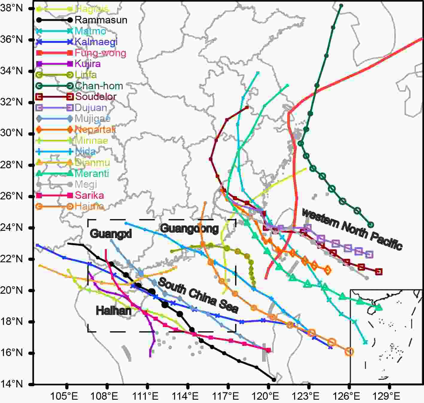
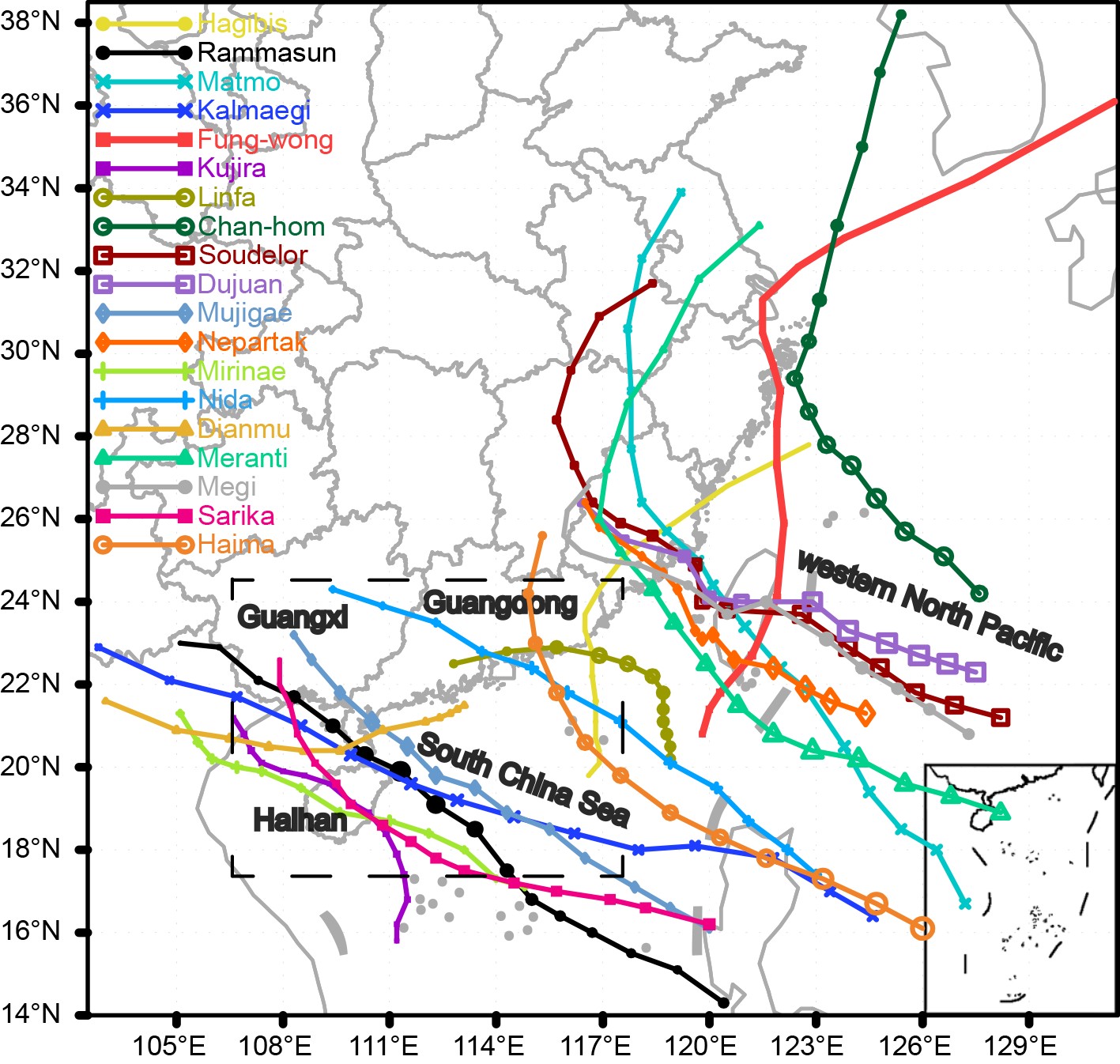
Figure 1. Tracks of the 19 TCs examined in this study from the CMA best-track analysis. Here, the TC position at the first forecast initialization time is used as the beginning of the track. The sizes of the TC symbols represent the TC intensities, with larger sizes corresponding to stronger TCs. The dashed rectangle indicates the region in the panels shown in Figs. 4, 6, and 14.
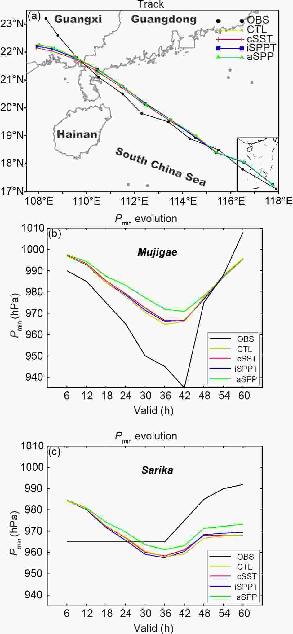
Figure 2. Forecasts of track (a) and Pmin (b) for typhoon Mujigae initialized at 1200 UTC 2 October 2015 and of Pmin (c) for typhoon Sarika initialized at 1200 UTC 16 October 2016. “OBS” represents the observation from CMA best-track dataset.
Initialization times TC names TC classifications Model domains 1200 13 Jun 2014 Hagibis Intensifying 99.52°–134.08°E, 5.92°–33.28°N 0000 14 Jun 2014 Hagibis Intensifying 99.72°–134.28°E, 6.32°–33.68°N 0000 16 Jul 2014 Rammasun Intensifying 103.32°–137.88°E, 0.8°–28.16°N 1200 16 Jul 2014 Rammasun Intensifying 100.52°–135.08°E, 1.82°–29.18°N 0000 17 Jul 2014 Rammasun Intensifying 98.62°–133.18°E, 2.72°–30.08°N 0000 21 Jul 2014 Matmo Intensifying 110.42°–144.98°E, 2.82°–30.18°N 1200 21 Jul 2014 Matmo Intensifying 108.12°–142.68°E, 4.82°–32.18°N 0000 22 Jul 2014 Matmo Non-intensifying 106.52°–141.08°E, 6.72°–34.08°N 0000 14 Sep 2014 Kalmaegi Intensifying 107.32°–141.88°E, 2.82°–30.18°N 1200 14 Sep 2014 Kalmaegi Intensifying 104.52°–139.08°E, 4.12°–31.48°N 0000 15 Sep 2014 Kalmaegi Intensifying 100.92° –135. 48°E, 4.32°–31.68°N 1200 20 Sep 2014 Fung-wong Non-intensifying 102.62°–137.18°E, 7.32°–34.68°N 0000 21 Sep 2014 Fung-wong Non-intensifying 102.92°–137.48°E, 8.12°–35.48°N 1200 21 Sep 2014 Fung-wong Non-intensifying 104.62°–139.18°E, 10.42°–37.78°N 0000 21 Jun 2015 Kujira Intensifying 94.22°–128.78°E, 2.52°–29.88°N 1200 21 Jun 2015 Kujira Intensifying 94.32°–128.88°E, 3.12°–30.48°N 0000 7 Jul 2015 Linfa Intensifying 101.72°–136.28°E, 6.72°–34.08°N 1200 7 Jul 2015 Linfa Intensifying 101.42°–135.98°E, 7.12°–34.48°N 0000 8 Jul 2015 Linfa Intensifying 101.32°–135.88°E, 7.72°–35.08°N 1200 9 Jul 2015 Chan-hom Intensifying 110.32°–144.88°E, 10.52°–37.88°N 0000 10 Jul 2015 Chan-hom Non-intensifying 108.22°–142.78°E, 12.02°–39.38°N 1200 6 Aug 2015 Soudelor Non-intensifying 110.92°–145.48°E, 7.52°–34.88°N 0000 7 Aug 2015 Soudelor Non-intensifying 108.52°–143.08°E, 8.12°–35.48°N 1200 7 Aug 2015 Soudelor Non-intensifying 106.62°–141.18°E, 9.22°–36.58°N 0000 27 Sep 2015 Dujuan Non-intensifying 110.32°–144.88°E, 8.62°–35.98°N 1200 27 Sep 2015 Dujuan Non-intensifying 108.62°–143.18°E, 9.12°–36.48°N 0000 28 Sep 2015 Dujuan Non-intensifying 106.72°–141.28°E, 9.62°–36.98°N 0000 2 Oct 2015 Mujigae Intensifying 102.72°–137.28°E, 2.42°–29.78°N 1200 2 Oct 2015 Mujigae Intensifying 100.62°–135.18°E, 3.42°–30.78°N 0000 3 Oct 2015 Mujigae Intensifying 98.42°–132.98°E, 4.82°–32.18°N 0000 7 Jul 2016 Nepartak Non-intensifying 107.22°–141.78°E, 7.62°–34.98°N 1200 7 Jul 2016 Nepartak Non-intensifying 105.42°–139.98°E, 8.22°–35.58°N 0000 8 Jul 2016 Nepartak Non-intensifying 103.42°–137.98°E, 8.82°–36.18°N 1200 25 Jul 2016 Mirinae Intensifying 98.12°–132.68°E, 3.22°–30.58°N 0000 31 Jul 2016 Nida Intensifying 105.72°–140.28°E, 3.72°–31.08°N 1200 31 Jul 2016 Nida Intensifying 103.82°–138.38°E, 5.02°–32.38°N 0000 17 Aug 2016 Dianmu Intensifying 95.42°–129.98°E, 7.42°–34.78°N 1200 12 Sep 2016 Meranti Intensifying 110.92°–145.48°E, 5.22°–32.58°N 0000 13 Sep 2016 Meranti Non-intensifying 108.32°–142.88°E, 5.92°–33.28°N 1200 13 Sep 2016 Meranti Non-intensifying 105.62°–140.18°E, 6.82°–34.18°N 0000 26 Sep 2016 Megi Intensifying 110.02°–144.58°E, 7.02°–34.38°N 1200 26 Sep 2016 Megi Non-intensifying 108.02°–142.58°E, 8.22°–35.58°N 0000 16 Oct 2016 Sarika Non-intensifying 102.72°–137.28°E, 2.52°–29.88°N 1200 16 Oct 2016 Sarika Non-intensifying 100.12°–134.68°E, 3.12°–30.48°N 0000 17 Oct 2016 Sarika Non-intensifying 97.52°–132.08°E, 3.52°–30.88°N 0000 19 Oct 2016 Haima Non-intensifying 108.72°–143.28°E, 2.42°–29.78°N 1200 19 Oct 2016 Haima Non-intensifying 105.92°–140.48°E, 3.62°–30.98°N 0000 20 Oct 2016 Haima Non-intensifying 103.02°–137.58°E, 4.52°–31.88°N Table 2. Description of the 48 forecasts carried out in this study, in terms of initialization times (UTC), TC names, TC classifications, and model domains. The words in boldface for TC classifications indicate the TC cases with RI.
-
Although adding spatially uncorrelated random perturbations to surface temperature (as in CTL) is a relatively simple way for creating an ensemble of SST, it ignores the spatial correlations in SST uncertainties (Torn, 2016). To investigate the impacts of spatial correlations in SST perturbations on TREPS, ensemble forecasts (cSST in Table 1) were conducted with spatially correlated SST perturbations. cSST is the same as CTL except that a random field drawn from a Gaussian distribution with a spatial decorrelation scale of l is added to surface temperature. Here, l is selected as the half of the initial wind radius of 17.2 m s−1 reported in the real-time warning information.
-
To address a drawback of the traditional SPPT that the same level of uncertainty is assigned to all atmospheric situations (Leutbecher et al., 2017), “independent SPPT” was proposed by Christensen et al. (2017) and has been confirmed to be effective for improving forecasts by increasing ensemble spreads in regions with evident convective activity. Inspired by Christensen et al. (2017), “f-inflated SPPT” was proposed here and used in the experiment named iSPPT (Table 1). In iSPPT, the multiplier f, which acts on the physical tendency and is used to form perturbed tendency in the SPPT scheme, is artificially inflated by fi in regions with evident convective activity to increase the perturbations there.
As illustrated in Ding (2005), the abundant low-level moisture, strong convective instability, and strong dynamical lifting are all essential to the occurrence of vigorous convective activity. So, the regions with vigorous convective activity can be roughly identified based on three metrics: the low-level moisture which can be represented by the specific humidity at 850 hPa (qv850), the convective instability which can be represented by the difference of equivalent potential temperature between 1000 hPa and 500 hPa (Diffθ), and the dynamical lifting which can be represented by the divergence of 850-hPa wind (Div850). Specifically, such regions can be identified if all the following three criteria are satisfied: (1) qv850 ≥ 14 g kg−1; (2) Diffθ ≥ 10 K; and (3) Div850 < 0 s−1. Note that the three criteria were based on both empirical estimation and tuning experimentation.
To be specific, fi is defined as
where Acon measures the intensity of convective activity and is calculated as
To avoid excessive perturbations causing numerical instability in regions far away from TCs, f is inflated only within 500 km of the TC center predicted by the control member, given that the significant convectively unstable regions are largely present around TCs.
-
The impacts of adding SPP are evaluated by combining SPP with SPPT and multi-physics in the experiment named aSPP (Table 1). The SPP scheme used here is similar to that implemented in Xu et al. (2020), where SPP was applied in a regional ensemble based on GRAPES with the focus of predictions in the East Asian monsoon region.
In SPP, the 14 key parameters that may have important impacts on TC forecasting are selected from MRF, YSU, Monin–Obukhov, WSM6, KF, and SAS. Table 3 gives the brief descriptions, default values, and ranges of the parameters selected. The parameters and their ranges are determined following recent literature (e.g., Baker et al., 2014; Zhang et al., 2014a; Di et al., 2015; Xu et al., 2020) and consultations with GRAPES physics parameterization experts. All the selected parameters are the same as those in Xu et al. (2020), with the exception of the three parameters used in the cumulus convection parameterizations. Note that the sensitivities of the selected parameters to TC forecasting were not investigated. Thus, the 14 perturbed parameters used in the SPP design may not be the most sensitive parameters greatly influencing TC forecasting. Further research is essential to select the most sensitive parameters to optimize the SPP design. Here, a brief explanation of the motivation behind selecting the parameters was given.
Scheme Parameter Description Default Range MRF Ric Critical Richardson number 0.25 [0.1, 0.75] MRF pfac Profile shape exponent for calculating the momentum
diffusivity coefficient2.0 [1, 3] MRF cfac Coefficient for Prandtl number 6.5 [3.4, 15.6] YSU Ric Critical Richardson number 0.1 [0.01, 0.5] YSU pfac Profile shape exponent for calculating the momentum
diffusivity coefficient2.0 [1, 3] YSU bfac Coefficient for Prandtl number 6.8 [3.4, 15.6] Monin-Obukhov XKA Molecular diffusivity (m2 s−1) 2.4×10⁻⁵ [1.2×10⁻⁵,
5.0×10⁻⁵]Monin-Obukhov CZO Charnock parameter 0.0185 [0.01, 0.026] WSM6 N0r Rain intercept parameter (m−4) 8.0×10⁶ [5.0×10⁶, 1.2×10⁷] WSM6 Nc Number concentration of cloud water droplet (m−3) 3.0×10⁸ [1.0×10⁷, 1.0×10⁹] WSM6 Ec Collection efficiency from cloud to rain auto conversion 0.55 [0.35, 0.85] KF R Cloud radius (m) R [0.9R, 1.1R] KF ee Coefficient for the minimum entrainment rate 0.5 [0.3, 0.7] SAS pgcon Proportionality constant for the convection-induced
pressure gradient force0.55 [0.3, 0.8] Notes: The identifiers of parameters are presented in the second column, with default values and empirically realistic ranges shown in the fourth and fifth columns, respectively. In KF, R is defined to vary with the magnitude of vertical velocity at the lifting condensation level. Table 3. Set-up of parameters used in the SPP scheme.
For the PBL parameterization, the PBL height is determined by the critical Richardson number (Ric) since Ric is an important criterion for the stability of PBL in both the MRF (Hong and Pan, 1996) and YSU (Hong et al., 2006) schemes. Both surface wind speed and rainfall have been proven to be very sensitive to Ric (Hong and Pan, 1996; Hong et al., 2006; Kepert, 2012; Wang et al., 2020). Additionally, the profile shape exponent for calculating the momentum diffusivity coefficient (pfac) in both MRF and YSU was selected, because pfac determines the mixing intensity of turbulent eddies, which is highly related to surface wind and rainfall (Aksoy et al., 2006; Di et al., 2015; Wang et al., 2020). The coefficient for Prandtl number at the top of the surface layer (cfac/bfac), which is used to calculate eddy diffusivity for temperature and moisture, shows some impacts on precipitation (Di et al., 2015). Ric, pfac, and cfac/bfac were thus selected for MRF/YSU.
In the Monin–Obukhov scheme, the multiplier for the heat/moisture exchange coefficient (XKA) is closely related to the strength of flux exchange and shows some impacts on precipitation and temperature (Di et al., 2015, 2017); while the Charnock parameter (CZO) is the multiplier for the roughness length, which converts wind speed to roughness length over sea and thereby determines the magnitude of the wind-speed dependent roughness length over sea (Baker et al., 2014). Therefore, XKA and CZO were selected here.
In WSM6, the intercept parameter (N0r) directly influences the entire drop-size distribution. Because the slope of distribution is proportional to intercept, the rain rate changes proportionally with N0r (Hacker et al., 2011a; Baker et al., 2014; Di et al., 2015). Both the number concentration of cloud water droplets (Nc) and the collection efficiency for the conversion of cloud water to rain (Ec) in WSM6 directly influences the transformation of cloud water to rainwater (Baker et al., 2014; Wang et al., 2020). N0r, Nc, and Ec were thus selected due to their important impacts on precipitation.
The cloud radius (R) and coefficient for the minimum entrainment rate (ee) are known to be uncertain and play crucial roles in KF (Kain and Fritsch, 1990; Kain, 2004). Simulated rainfall has been shown to be sensitive to both R and ee (Zhang et al., 2014a). As such, the parameters R and ee are selected for KF. The proportionality constant for the convection-induced pressure gradient force (pgcon) has been shown in Zhang and Wu (2003) to vary with the height and shows significant impacts on forecast performance (Han and Pan, 2006; Han et al., 2020). The parameter pgcon is thus selected for SAS.
The perturbations used in SPP are introduced as
where
$ \xi ' $ and$ \xi $ denote the perturbed and unperturbed parameters, respectively; and r denote a random field drawn from a Gaussian distribution with spatial and temporal decorrelations. The selected 14 key parameters are stochastically perturbed at each time step and the random fields r for different parameters are independent. The spatial and temporal decorrelation scales of random fields r used in SPP are the same as those used in SPPT. The perturbed parameters are kept within strictly specified bounds, as indicated by the ranges of parameters in Table 3, to prevent them from attaining physically unrealistic values. -
The impacts of the spatially correlated SST perturbations, f-inflated SPPT, and adding SPP on TREPS are evaluated by comparing cSST, iSPPT, and aSPP with CTL, respectively, for both deterministic and probabilistic guidance. Since CTL was actually the retrospective forecasts conducted in Z18, the verification metrics used in this study are the same as those in Z18, where the detailed descriptions of verification metrics were given, and are briefly presented in Table 4.
Metric Acronym Description Perfect Range Absolute track/intensity error Error The absolute error of the ensemble-mean track/intensity forecasting 0 [0, +∞) Threat score TS The accuracy in predicting the area of variable over a given threshold 1 [0, 1] Fractions skill score FSS The spatial skill calculated based on observed and predicted fractions over a neighborhood size 1 [0, 1] Reliability aspect of Brier score BSrely The agreement between predicted probability and mean observed frequency 0 [0, +∞) Area under the relative operating characteristic curve AROC The ability of a forecast to discriminate between two alternative outcomes 1 [0, 1] Table 4. Description of metrics used in the verification.
The deterministic guidance includes the ensemble-mean track (the TC center position) and intensity, which includes the TC minimum central pressure (Pmin) and maximum sustained wind speed (Vmax), respectively, as well as the probability-matched mean (PM; Ebert, 2001) 10-m wind speed and 1-h accumulated rainfall. The probabilistic guidance includes the probability of 10-m wind speed and 1-h accumulated rainfall at different thresholds. The forecasts of 10-m wind speed exceeding 17.2 and 24.5 m s−1, which are respectively named modest and strong winds hereafter, are verified. The forecasts of 1-h accumulated rainfall are verified for the thresholds of 0.1, 5, and 15 mm, which are respectively named light, moderate, and heavy rainfall hereafter.
As in Z18, the TC center is defined as the minimum of the 850-hPa geopotential height. Following Torn (2010), Pmin is defined as the lowest sea level pressure within 100 km of the TC center, while Vmax is defined as the largest 10-m wind speed within 250 km of the TC center. The ensemble-mean track, Pmin, and Vmax are calculated as the average of the TC center positions, Pmin, and Vmax from the 30 perturbed forecasts, respectively. The CMA best-track dataset (Ying et al., 2014; Lu et al., 2021;
http://tcdata.typhoon.org.cn ) was used to calculate the average absolute track error and intensity error. This dataset includes some important information related to TCs having passed through the western North Pacific (WNP) and the South China Sea (SCS) since 1949, such as track, intensity, dynamic and thermal structures, wind strengths, and precipitation. For fair comparisons, a homogeneous sample of TC cases with predicted or observed Vmax above 10 m s−1 was used.Forecasts of 10-m wind speed and 1-h accumulated rainfall were verified against the 6-hourly 10-m wind and hourly rainfall observations, respectively, from the automatic weather stations over the Chinese mainland. The observations were interpolated to the NWP model grids using Cressman interpolation to calculate skill scores. As in Z18, the verification area and period for both wind and rainfall are defined as the domain and time directly influenced by TC, respectively. The threat score (TS; Gilbert, 1884) and fraction skill score (FSS; Roberts and Lean, 2008) were used to verify the deterministic guidance for 10-m wind speed and 1-h accumulated rainfall, respectively. For FSS, the 50-km neighborhood length was used in this study. For both TS and FSS, the larger values indicate higher forecast skills. Probabilistic guidance was verified by calculating the reliability aspect of Brier score (BSrely; Candille and Talagrand, 2005) and the area under the relative operating characteristic curve (AROC; Mason and Graham, 2002). A smaller BSrely indicates better reliability, while a greater AROC indicates better discriminating ability.
The relative changes in skill scores for a particular experiment (i.e., cSST, iSPPT, and aSPP) with respect to CTL were discussed here to investigate the differences in forecast performance among various experiments, as in Montmerle et al. (2018) and Caron et al. (2019). Specifically, relative changes in the absolute track/intensity error, TS, FSS, BSrely, and AROC, which were hereafter expressed as ΔError, ΔTS, ΔFSS, ΔBSrely, and ΔAROC, respectively, were calculated. For the comparison of skill scores, statistical significances of the differences between different ensemble experiments were assessed using a bootstrap resampling procedure (Davis et al., 2010), which was repeated 1000 times. As in Zhang (2018b), only results above the 85% or 90% significance level (indicating an 85 or 90% probability that two skill scores differed) are labelled.
-
For the 19 TC cases examined in this study, most of them formed in WNP and moved northwestward to make landfall on the coastal areas of southeast China; several of them formed in SCS and mainly made landfall on the Guangxi, Guangdong, and Hainan provinces (Fig. 1).
-
Because the rapid intensification (RI) of TCs is characterized by large forecast uncertainty or low predictability (Zhang and Tao, 2013; Emanuel and Zhang, 2016; Judt and Chen, 2016), accurately predicting TC cases with RI remains a major challenge (Rappaport et al., 2012; Rogers et al., 2013; Judt and Chen, 2015). Thus, the impacts of new implementing strategies for perturbations are evaluated for forecasts of TC cases with significant and insignificant intensification stage, respectively.
The 19 TC cases examined in this study were discriminated in terms of intensity evolution (Fig. 1). The observed 24-h changes in Vmax were calculated based on the CMA best-track dataset throughout the 60-h forecasts for each of the 48 forecasts. The TC cases were defined as intensifying TCs if the observed 24-h TC intensification rates were larger than 5 m s−1 at least once during the 60-h forecasts; while the other TC cases were defined as non-intensifying TCs. According to the definition, 25 and 23 forecasts were classified as forecasts of intensifying and non-intensifying TCs, respectively, among the 48 forecasts (Table 2). Among the 25 forecasts of intensifying TCs, there were six forecasts classified as forecasts of the TC cases with RI (Table 2), which were identified if the observed 24-h TC intensification rates were above 15 m s−1 at least once during the 60-h forecasts (Emanuel, 2018). However, the impacts of the three new implementing strategies for perturbations on TCs with RI were generally similar to those on intensifying TCs and were thus not separately shown in the verification metrics.
-
Two of the 48 forecasts with initial times of 1200 UTC 2 October 2015 and 1200 UTC 16 October 2016 (i.e., typhoons Mujigae and Sarika, respectively) were selected to intuitively demonstrate the representative characteristics of ensemble forecasts in the intensifying and non-intensifying TCs, respectively (Fig. 2).
Typhoon Mujigae entered the South China Sea at 0200 UTC 2 October 2015 (Fig. 2a) and underwent RI with Vmax increasing from 28 (at 0600 UTC 3 October) to 52 (at 0600 UTC 4 October) m s−1. Mujigae made landfall on Guangdong at around 0600 UTC 4 October 2015 with Pmin of 935 hPa (Fig. 2b). Mujigae is the strongest TC making landfall on Guangdong in October since 1949 and caused severe flooding and several TC-spawned tornadoes, resulting in significant disaster in Guangdong (Bai et al., 2017).
Typhoon Sarika entered the South China Sea at around 0600 UTC 16 October 2016 and then moved northwestward. Pmin and Vmax of Sarika held steadily at 965 hPa and 38 m s−1, respectively, from 0600 UTC 16 October to 0000 UTC 18 October, when Sarika made landfall on Hainan (Fig. 2c). Sarika is the strongest TC making landfall on Hainan in October since 1971 and resulted in great damage in Hainan, Guangdong, and Guangxi, due to its heavy rainfall and strong winds (Gu et al., 2017).
-
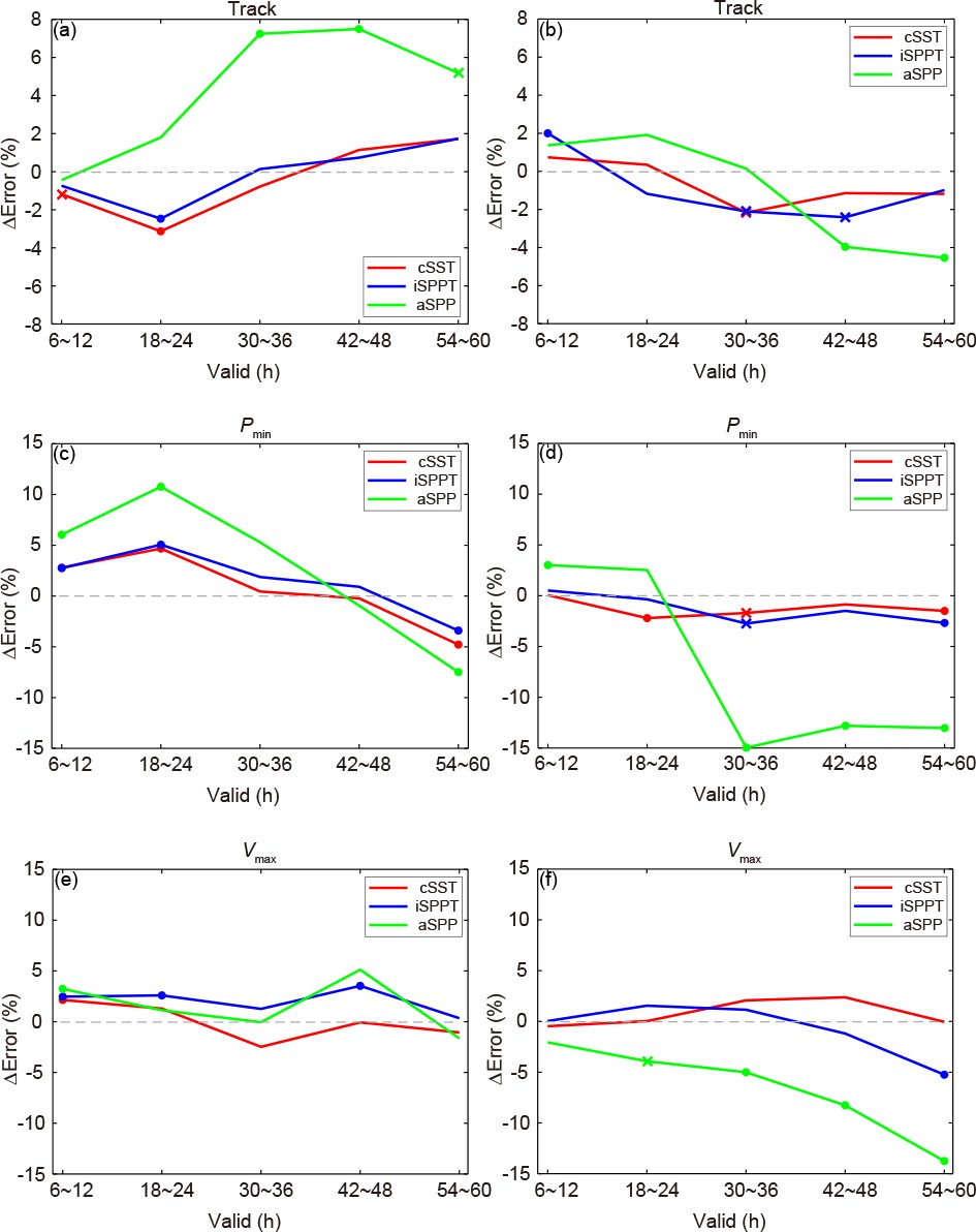
ΔError of cSST with respect to CTL in Figs. 3a, b shows that the ensemble-mean track forecasts were improved at most lead times due to implementing spatial correlations in SST perturbations. This result is also intuitively shown in Fig. 2a. However, the impacts of the spatially correlated SST perturbations on the ensemble-mean intensity forecasts were mixed. For intensifying TCs, cSST was generally comparable to CTL in both Pmin and Vmax forecasting (Figs. 3c, e); while for non-intensifying TCs, improvements of cSST over CTL were statistically significant in Pmin forecasting (Fig. 3d). The performance of iSPPT was overall similar to that of cSST in both track and intensity forecasting except that iSPPT degraded and improved intensity forecasting relative to cSST for intensifying and non-intensifying TCs, respectively (Figs. 3c–f).
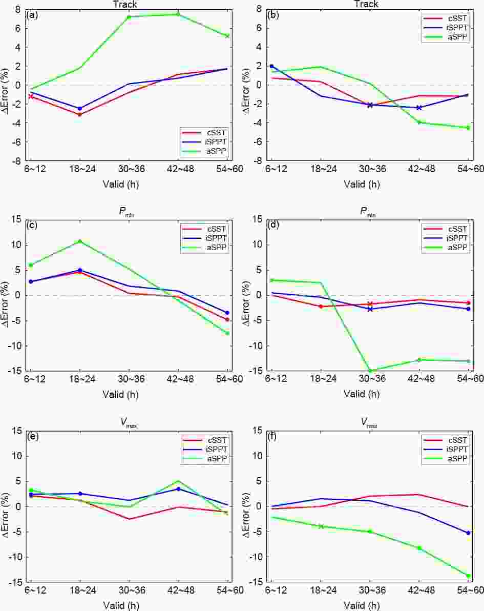
Figure 3. The relative changes in absolute errors (ΔError) of the TC track (a, b), Pmin (c, d), and Vmax (e, f) averaged over different lead times for intensifying (left column) and non-intensifying (right column) TCs. ΔError is calculated for a particular experiment (name in the legend) with respect to “CTL”. The dots (crosses) on the curves indicate the lead times for which the significance level of ΔError is larger than 90% (85%).
Note that both SST perturbations and f-inflated SPPT are implemented only in areas around the TC. As such, the impacts of the spatially correlated SST perturbations and f-inflated SPPT may be limited in areas far away from the TC inner core. Some recent research has shown that RI of TCs is associated with the complex multiscale interactions among the surrounding environment, TC vortex, and internal convective processes (e.g., Rogers et al., 2015; Judt et al., 2016; Judt and Chen, 2016). Thus, the localized impacts of the spatially correlated SST perturbations and f-inflated SPPT are likely limited in improving the description of uncertainties related to the interactions among multiscale processes, leading to limited improvements in forecasting intensifying TCs. As RI of TCs is often accompanied by the occurrence of convective bursts (Rogers et al., 2013; Wang and Wang, 2014; Tang et al., 2018), the fact that SPPT is limited in representing the uncertainties in triggering of convection (Tompkins and Berner, 2008; Bengtsson et al., 2021) may limit the improvements of iSPPT in forecasting intensifying TCs. Moreover, inflating f in the SPPT scheme only around the TC may lead to unexpected discontinuity in the physical tendency, which is probably detrimental to improve the uncertainty description especially for the multiscale-process interactions. This insufficiency may explain why iSPPT underperformed CTL in forecasting intensifying TCs (Figs. 3c, e) and should be addressed in future work.
Compared with CTL, aSPP showed degradations in both track and intensity forecasting for intensifying TCs at most lead times (Figs. 3a, c, e); but the opposite was true for non-intensifying TCs (Figs. 3b, d, f). In particular, the maximum ΔErrors of aSPP relative to CTL for Pmin of intensifying and non-intensifying TCs were around 10% and -10%, respectively (Figs. 3c, d). Such ΔError is related to the change in intensity biases. For intensifying TCs, CTL showed weak biases in intensity forecasting before TC making landfall (Fig. 2b); while for non-intensifying TCs, CTL showed strong biases in intensity forecasting during most of the TC lifetime (Fig. 2c). Thus, compared with CTL, aSPP predicted weaker TCs and thereby aggravated the intensity underestimation for intensifying TCs but alleviated the intensity overestimation for non-intensifying TCs (Figs. 2b, c), leading to case-dependent intensity ΔErrors.
To investigate the reason why adding SPP causes weak biases in intensity forecasting, deterministic forecasts for the case study of typhoon Mujigae (2015) were carried out with different settings for the 14 perturbed parameters. For most of the perturbed parameters, the impacts of perturbing their values on surface wind were generally consistent with those of perturbing Ric. For this reason, only the results of perturbing Ric in YSU are shown here. Specifically, Ric was inflated by 2.5 and 1/2.5 relative to the default setting of 0.1, respectively. Ric is used to determine the stability of PBL, and increasing Ric tends to reduce the stability criterion in PBL. Therefore, increased Ric indicates more unstable PBL. Non-local momentum mixing will be activated in the unstable PBL. Such enhanced momentum mixing leads to enhanced surface wind speed (Brown and Grant, 1997). It is thus not surprising that increasing Ric from 0.1 to 0.25 tended to strengthen 10-m wind outside the TC inner core (Fig. 4b). However, the enhanced momentum mixing should cause a smoother wind field at the TC eyewall and thereby weaken the TC intensity (Kepert, 2012). As such, increasing Ric from 0.1 to 0.25 tended to weaken 10-m wind near the TC inner core (Fig. 4b). Because increasing (decreasing) Ric tends to enhance (reduce) the impacts of non-local turbulence mixing, which are characterized by evident nonlinearity (Brown and Grant, 1997), it should be expected that increasing (decreasing) Ric causes larger (smaller) impacts on surface wind field. Thus, increasing Ric from 0.1 to 0.25 (Fig. 4b) generally led to larger changes in surface wind field than decreasing Ric from 0.1 to 0.04 (Fig. 4a). Similarly, increasing (decreasing) pfac caused reductions (enhancements) in momentum mixing, leading to smaller (larger) impacts on surface wind field (not shown). These imply that the change in surface wind field with Ric or pfac may be nonlinear although monotonic. Thus, perturbing Ric or pfac in a way like (3) was apt to weaken TC intensity but strengthen surface wind outside the TC inner core. Further work is required to address such biases.
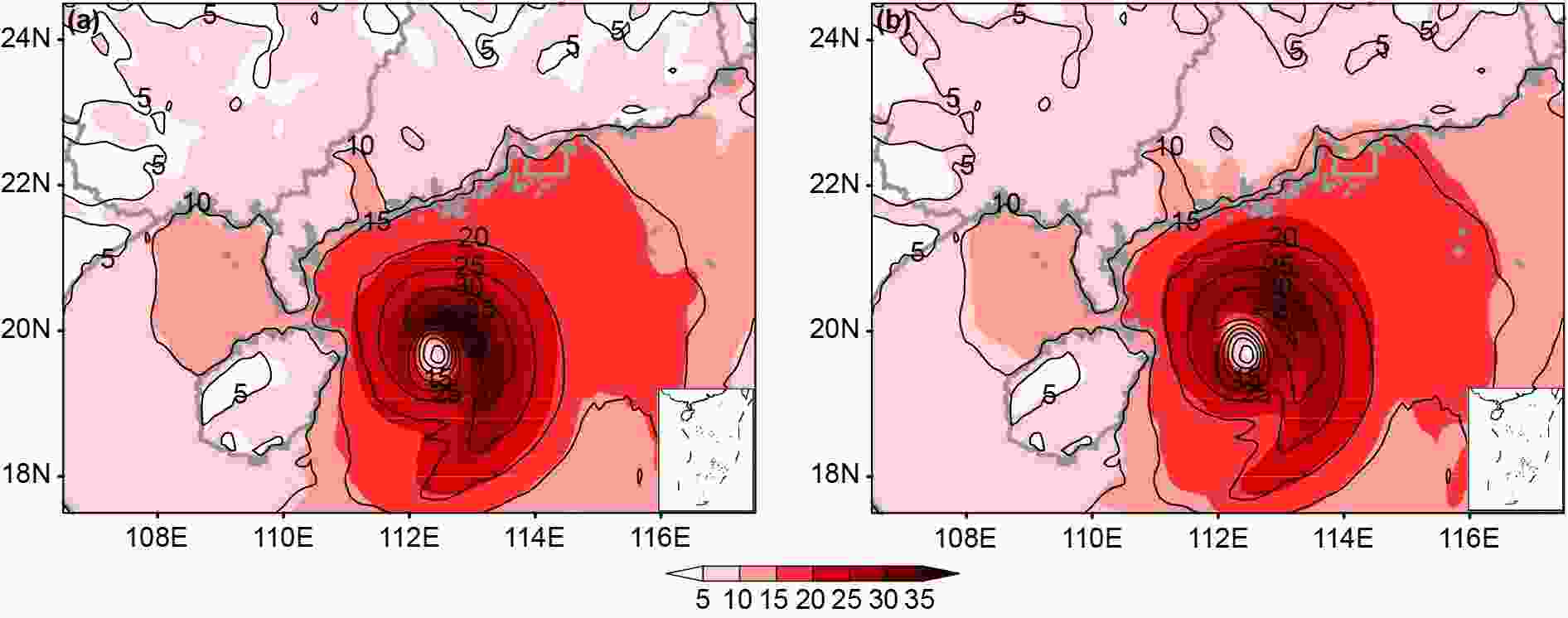
Figure 4. 30-h forecasts of 10-m wind (units: m s−1) from the deterministic forecasts initialized at 1200 UTC 2 October 2015, with the critical Richardson number (Ric) of 0.1 (contour with interval of 5 m s−1), is changed to (a) 0.04 and (b) 0.25. The range of panels is the same as the dashed rectangle shown in Fig. 1.
Note that the impacts of perturbing some of the parameters (e.g., R and ee in KF) on 10-m wind outside the TC inner core were inconsistent with those of perturbing Ric or pfac (not shown). However, the impacts of perturbing Ric and pfac dominated the combined impacts of simultaneously perturbing all the 14 parameters.
-
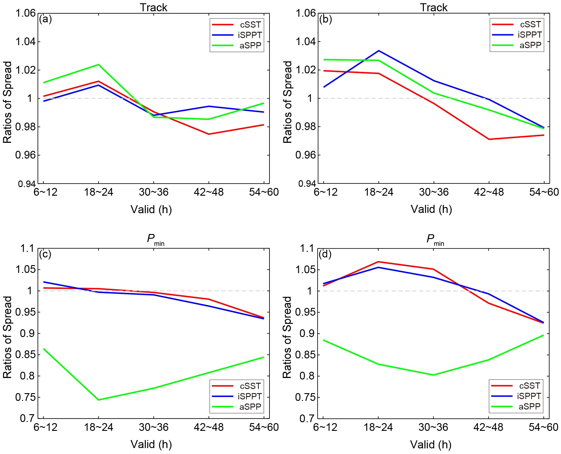
As illustrated in Z18, according to the conditions that must be satisfied to issue TREPS, the lead time when TC made landfall mainly lies between 24 and 54 h. Figure 5 indicates that cSST and iSPPT generally increased ensemble spreads over CTL in both track and intensity before TC making landfall. This result was more evident for non-intensifying than intensifying TCs, again illustrating the larger insufficiency of the spatially correlated SST perturbations and f-inflated SPPT in improving the uncertainty description of intensifying than non-intensifying TCs.
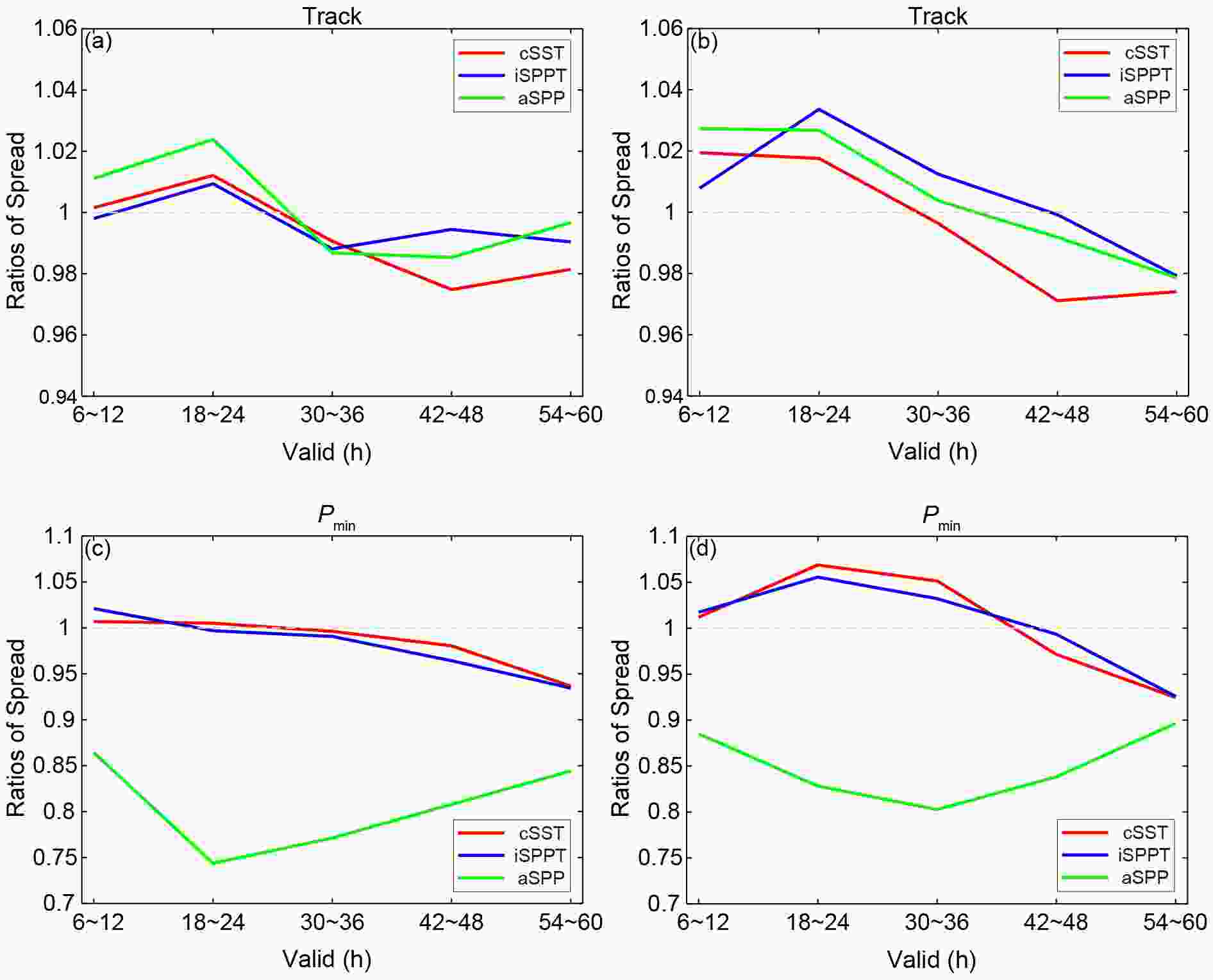
Figure 5. The ratios of ensemble spread of a particular experiment (name in the legend) to ensemble spread of CTL for the TC track (a, b) and Pmin (c, d) averaged over different lead times for intensifying (left column) and non-intensifying (right column) TCs.
Compared with CTL, because the position spreading of TC center in ensemble members was more evident in cSST, iSPPT, and aSPP before TC making landfall, TCs in some ensemble members of cSST, iSPPT, and aSPP made landfall earlier (cf. white dots in Fig. 6a with those in Figs. 6b–d). These ensemble members with earlier TC landfall were characterized by earlier TC decaying due to the process of landfall. Such behavior was more prominent for TCs with more evident intensification. As a result, compared with CTL, there was larger ensemble-mean Pmin around landfall time in cSST, iSPPT, and aSPP for intensifying TCs (Fig. 2b), leading to larger weak biases and thereby to larger intensity errors (Fig. 3c).
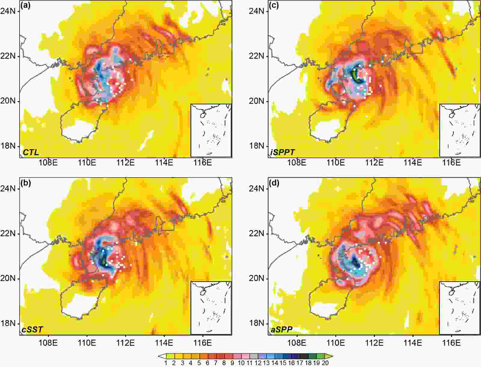
Figure 6. Distributions of the 36-h predicted TC center positions (white dots) and 39-h predicted ensemble spreads of 1-h accumulated precipitation (shading, mm) of the perturbed forecasts initialized at 1200 UTC 2 October 2015. The range of panels is the same as the dashed rectangle shown in Fig. 1.
After TC making landfall, cSST and iSPPT decreased ensemble spreads over CTL in both track and intensity, with earlier spread reductions in intensifying than non-intensifying TCs (Fig. 5). This may be because cSST and iSPPT had more ensemble members in which landfalling TCs had dissipated compared to CTL. Moreover, iSPPT showed larger track spreads than cSST especially beyond 18 h (Figs. 5a, b), because f-inflated SPPT is implemented above the PBL where steering flows prevail while SST perturbations is implemented only at the surface.
aSPP decreased intensity spreads compared with CTL in the entire 60-h forecasts (Figs. 5c, d), chiefly due to the weak biases of SPP. Such weak biases tend to generate more ensemble members in which landfalling TCs had dissipated in aSPP than iSPPT, which partially explained why aSPP generally showed larger track spreads before 24 h but smaller track spreads thereafter than iSPPT (Figs. 5a, b).
-
As shown in solid curves in Figs. 7a, b, cSST and iSPPT decreased the root-mean-square errors (RMSEs) of ensemble-mean 10-m wind relative to CTL. Overall, the ratio of wind spreads of cSST or iSPPT to CTL (dashed curves in Figs. 7a, b) evolved similarly with that of track or intensity spreads shown in Fig. 5. Compared with CTL, cSST and iSPPT generally increased wind spreads before TC making landfall for non-intensifying TCs but slightly decreased wind spreads before 24 h for intensifying TCs. Because wind spreads were calculated in the verification area, which was a specific domain covering the main region of observed rainfall and wind related to TCs on land, larger track spreads in cSST and iSPPT than CTL in the first few hours of forecasts may have resulted in less ensemble members in which the outer wind fields of TCs had covered the verification area. In this case, compared with CTL, cSST and iSPPT were characterized by lower frequency of points with nonzero wind speed, leading to a reduction in the ensemble standard deviation of wind. This behavior seemed to be more prominent in rainfall than wind and was intuitively shown in Fig. 6. Specifically, comparted with CTL, both cSST and iSPPT showed larger spreads of 1-h accumulated rainfall on the sea but smaller spreads on land (cf. shading among Figs. 6a–c). Thus, it should not be surprising that cSST and iSPPT decreased rainfall spreads compared with CTL before 24 h for intensifying TCs (Fig. 7c). In general, cSST and iSPPT showed comparable RMSEs of ensemble-mean rainfall relative to CTL (Figs. 7c, d).

Figure 7. As in Fig. 5, but for the ratios of RMSE of ensemble mean (solid) and ensemble spread (dashed) for 10-m wind (a, b) and 1-h accumulated precipitation (c, d).
Compared with CTL, aSPP increased RMSEs of ensemble-mean wind due to the strong biases of wind outside the TC inner core, with more evident RMSE increases in non-intensifying than intensifying TCs (Figs. 7a, b). SPP increased the frequency of points with nonzero wind speed, which showed up as an increase in wind spreads, especially for non-intensifying TCs (Fig. 7b). Note that wind spreads beyond 42 h in intensifying TCs were smaller in aSPP than CTL. This behavior was associated with the previously illustrated result that there were more ensemble members in which landfalling TCs had dissipated in aSPP than CTL in intensifying TCs. Unlike wind, rainfall did not suffer from any clear biases due to adding SPP (not shown). This is because, although the impacts due to perturbing parameters on rainfall differed among the 14 parameters, these diverse impacts compensated each other when the 14 parameters were simultaneously perturbed. The ensemble-mean rainfall was overall comparable between aSPP and CTL in terms of RMSEs (Figs. 7c, d). However, aSPP slightly degraded rainfall RMSEs over CTL for non-intensifying TCs beyond 36 h, perhaps due to wind biases. The ratio of rainfall spreads of aSPP to CTL behaved differently with that of wind spreads. To be specific, aSPP prominently increased rainfall spreads over CTL for all TC cases (Figs. 7c, d). The comparison between Figs. 6a and d shows that rainfall spreads were larger in aSPP than CTL in both the sea and land. This indicates that the SPP scheme used in this study can effectively improve rainfall spreads without evidently degrading the ensemble-mean rainfall.
-
In all TC cases, cSST and iSPPT were on average more skillful in PM of 10-m wind than CTL for both modest and strong winds (Fig. 8). This result can mainly be attributed to the improved forecasts of spatial pattern of wind field of cSST and iSPPT over CTL, since cSST and iSPPT outperformed CTL in ensemble-mean wind (Figs. 7a, b). However, for non-intensifying TCs, the increased wind spreads of cSST and iSPPT over CTL before TC making landfall (Fig. 7b) should also contribute to the improved PM wind especially for strong winds (Fig. 8d), which is often underestimated by the deterministic forecasts of TREPS (not shown). The performance of PM wind of cSST was generally comparable to that of iSPPT except that cSST significantly improved PM wind over iSPPT for strong winds in intensifying TCs before 30 h when cSST was found to increase wind spreads over iSPPT (Fig. 7a).

Figure 8. As in Fig. 3, but for the relative changes in TS (ΔTS) of the forecasts of 10-m wind with thresholds of (a, b) 17.2 and (c, d) 24.5 m s−1, and the relative changes in FSS (ΔFSS) of the forecasts of 1-h accumulated precipitation with threshold of (e, f) 5 mm.
Given that the FSS differences in PM rainfall among the four experiments are statistically insignificant during the entire 60-h forecasts for both light and heavy rainfall, only the results for moderate rainfall are shown here. Compared with PM rainfall of CTL, that of cSST and iSPPT on average showed better skills in terms of FSS for moderate rainfall (Figs. 8e, f). However, the positive ΔFSSs of cSST or iSPPT relative to CTL were statistically significant only at partial lead times. The limited impacts of the spatially correlated SST perturbations and f-inflated SPPT on rainfall forecasting were related to their insufficient effects in increasing rainfall spreads (Figs. 7c, d).
Recall from Figs. 7a, b that aSPP degraded ensemble-mean wind over CTL due to the strong biases of surface wind outside the TC inner core, with more prominent degradations in non-intensifying than intensifying TCs before TC making landfall. It should thus be expected that the superiority of aSPP to CTL in PM wind was more significant for modest winds, which is the major component of surface wind outside the TC inner core, in intensifying than non-intensifying TCs before 36 h (Figs. 8a, b). In contrast, aSPP outperformed CTL in PM wind more significantly for strong winds in non-intensifying than intensifying TCs (Figs. 8c, d). This is related to the more evident spread increases of aSPP over CTL in non-intensifying than intensifying TCs (Figs. 7c, d).
In all TC cases, PM rainfall of aSPP overall showed higher FSSs compared with that of CTL for moderate rainfall at most lead times (Figs. 8e, f). However, ΔFSSs of aSPP relative to CTL were statistically less significant for intensifying than non-intensifying TCs. Such result is chiefly attributable to the comparable performance in ensemble-mean rainfall between aSPP and CTL for intensifying TCs (Fig. 7c). The result that aSPP evidently increased rainfall spreads over CTL for non-intensifying TCs (Fig. 7d) contributes to the significant superiority of aSPP PM in moderate rainfall.
-
Figures 9a and b indicate that CTL overforecasted at probabilities above 25% for both modest winds and moderate rainfall, with more prominent overconfidence for non-intensifying than intensifying TCs and for wind than rainfall. Actually, CTL underforecasted at probabilities below 25% especially for intensifying TCs (Fig. 9a).
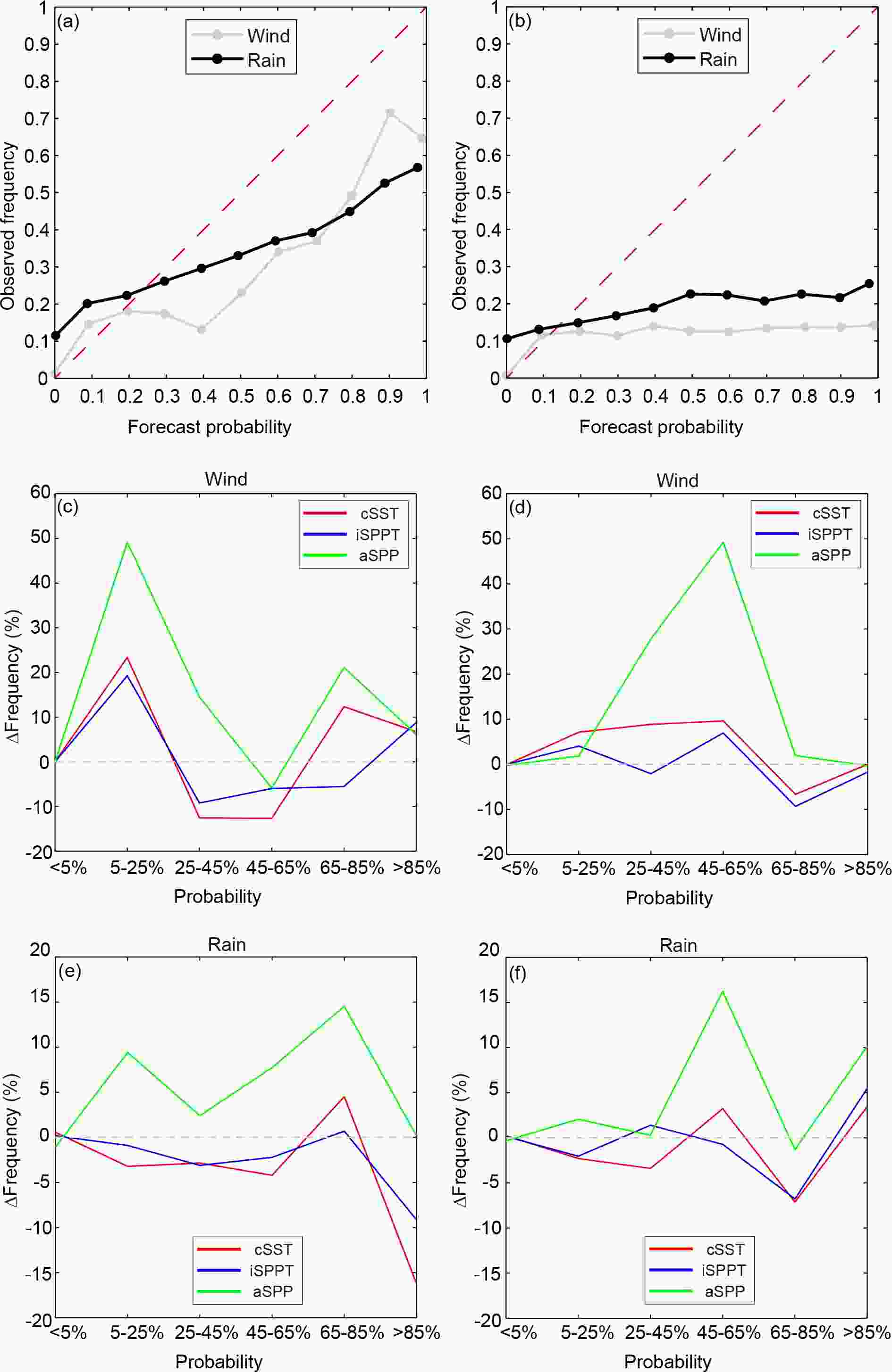
Figure 9. (a, b) Reliability diagram for 10-m wind (gray) and 1-h accumulated precipitation (black) of CTL with probability classes indicated by dots. The relative changes in frequency of probabilistic event occurrence (ΔFrequency) are shown for (c, d) 10-m wind and (e, f) 1-h accumulated precipitation. The results are shown for 10-m wind with the threshold of 17.2 m s−1 averaged over 6 and 12 h and for 1-h accumulated precipitation with the threshold of 5 mm averaged over 25–36 h for intensifying (left column) and non-intensifying (right column) TCs.
The slightly reduced wind spreads of cSST and iSPPT over CTL for intensifying TCs before landfall time (Fig. 7a) decreased coverages of moderate probabilities (25%–65%) but increased coverages of higher (>65%) and lower (<25%) probabilities (Fig. 9c). Thus, compared with CTL, cSST and iSPPT alleviated underforecasting at probabilities below 25%, alleviated overforecasting at probabilities of 25%–65%, but aggravated overforecasting at probabilities above 65% for modest winds of intensifying TCs before landfall. In particular, compared with cSST, iSPPT increased wind spreads over CTL for intensifying TCs before landfall more evidently (Fig. 7a), leading to more moderate-to-high-probability (65%–85%) events being translated into higher-probability (>85%) events for modest winds (Fig. 9c). Given the larger contributions of higher-probability events to probabilistic fields before TC making landfall (not shown), cSST and iSPPT degraded reliability over CTL for modest winds of intensifying TCs before 24 h, with more evident degradations in iSPPT than cSST (Fig. 10a). Conversely, both cSST and iSPPT were significantly more reliable than CTL for modest winds of non-intensifying TCs before 24 h (Fig. 10b). This is because the enhanced wind spreads of cSST and iSPPT over CTL for non-intensifying TCs before landfall time (Fig. 7b) decreased coverages of higher probabilities but increased coverages of lower probabilities (Fig. 9d), leading to alleviation in overforecasting for modest winds.

Figure 10. As in Figs. 8a–d, but for the relative changes in BSrely (ΔBSrely).
After TC making landfall, contributions of lower-probability events to probabilistic fields increased with lead times (not shown). Therefore, compared with CTL, the reduced wind spreads of cSST and iSPPT for intensifying TCs after landfall time (Fig. 7a) improved reliability for modest winds beyond 30 h, with more evident improvements in iSPPT than cSST (Fig. 10a). However, there were no statistically significant differences in BSrely between cSST or iSPPT and CTL for modest winds of non-intensifying TCs beyond 30 h, when the corresponding differences in wind spreads (especially between iSPPT and CTL) were also limited (Fig. 7b). Thus, both cSST and iSPPT were on average more reliable than CTL for modest winds during the entire 60-h forecasts.
The advantages of cSST and iSPPT for reliability of prediction of strong winds were generally similar to those for modest winds except that cSST degraded the strong-wind reliability for non-intensifying TCs before 24 h but significantly improved it thereafter over CTL (Fig. 10d). This is perhaps because cSST decreased wind spreads over CTL for non-intensifying TCs after landfall time (Fig. 7b) and thereby alleviated the serious overforecasting at higher probabilities for strong winds (not shown).
Compared with CTL, the strong biases of surface wind outside the TC inner core of aSPP resulted in more frequent occurrences of modest winds for all TC cases (Figs. 9c, d), leading to slightly worse reliability (Figs. 10a, b). Strong winds largely occurs near the TC inner core, where aSPP was characterized by weak biases of surface wind. As such, the overforecasting of CTL at higher probabilities for strong winds was alleviated in aSPP (not shown), leading to significant improvements of aSPP over CTL in strong-wind reliability around landfall time (Figs. 10c, d).
In terms of light rainfall, cSST and iSPPT generally showed comparable reliability compared with CTL (Figs. 11a, b). For moderate rainfall around and after landfall time, compared with CTL, cSST and iSPPT decreased rainfall spreads (Figs. 7c, d) and thus decreased coverages of probabilities of 5%–85% (Figs. 9e, f), leading to alleviation of overforecasting at most probabilities for all TC cases. Thus, cSST and iSPPT were on average more reliable than CTL for moderate rainfall beyond 13 h (Figs. 11c, d). As illustrated in section 4.1.3, for intensifying TCs around and after landfall time, the reduced rainfall spreads of cSST or iSPPT over CTL were related to the reduced frequency of points with nonzero rainfall. In this case, compared with iSPPT, cSST was characterized by smaller rainfall spreads (Fig. 7c). It is thus expected that cSST reduced occurrence frequency of rainfall over CTL more prominently than iSPPT, especially for higher-probability (>85%) events (Fig. 9c). However, the statistically significant differences in reliability between cSST and CTL were mainly present in heavy rainfall, with reliability improvements and degradations of cSST over CTL in intensifying and non-intensifying TCs, respectively (Figs. 11e, f). This may be associated with the decreased rainfall spreads of cSST over CTL for intensifying TCs (Fig. 7c), which were beneficial to alleviating overforecasting at higher probabilities for heavy rainfall. For similar reasons, cSST was more reliable than iSPPT for heavy rainfall of intensifying TCs (Fig. 11e). The increased rainfall spreads of cSST over CTL for non-intensifying TCs were present in 13–24 h (Fig. 7d), which can aggravate overforecasting at higher probabilities for heavy rainfall but cannot completely explain the significant reliability degradations of cSST over CTL beyond 36 h. Such degradations need further investigations in future work.
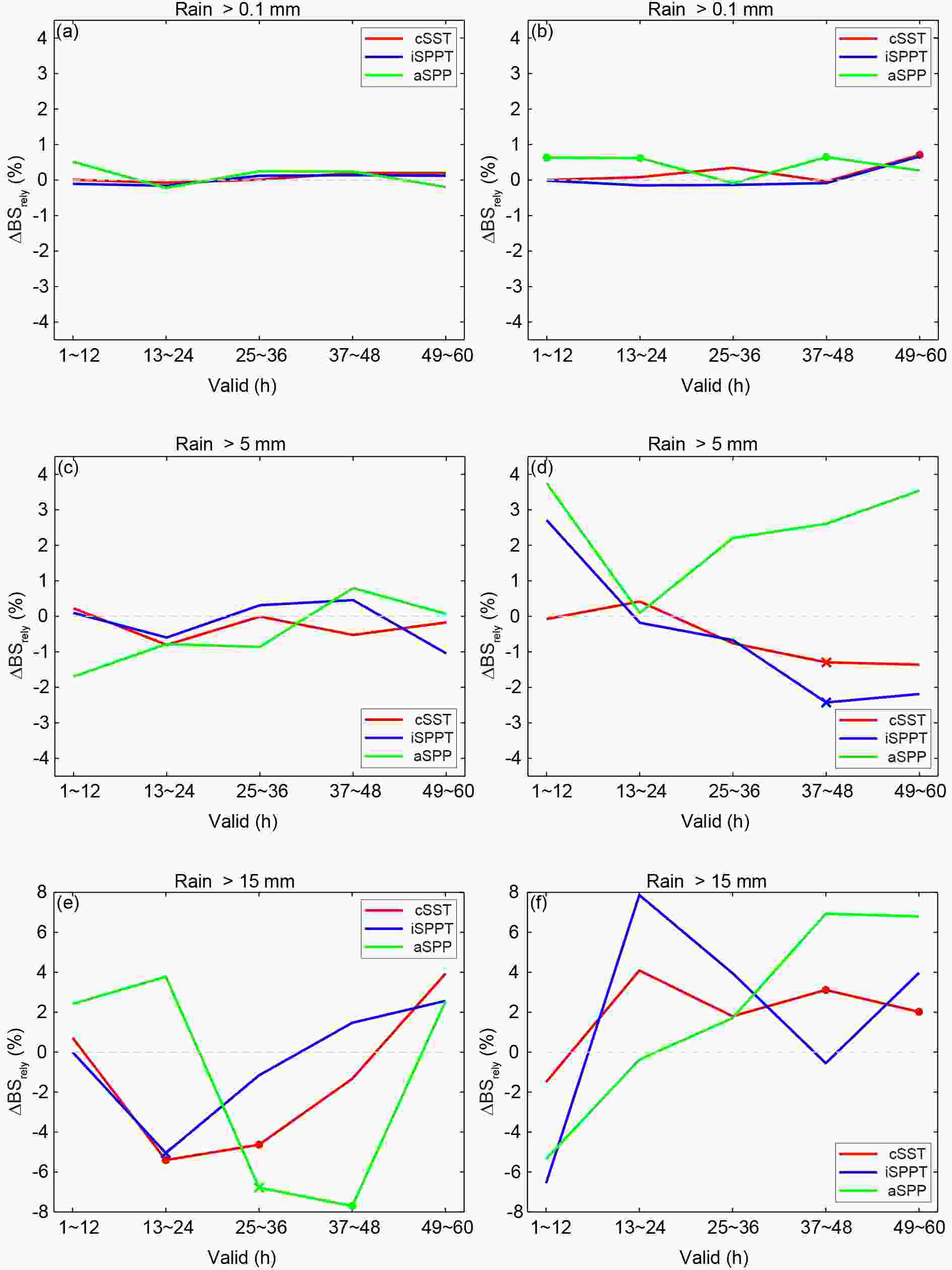
Figure 11. As in Figs. 8e, f, but for the relative changes in BSrely (ΔBSrely) of the forecasts of 1-h accumulated precipitation with thresholds of (a, b) 0.1, (c, d) 5, and (e, f) 15 mm.
Overall, aSPP degraded reliability for light rainfall over CTL, especially for non-intensifying TCs (Fig. 11b). aSPP increased occurrence frequencies of moderate rainfall over CTL at most probabilities for all TC cases, which indicates the wetting effect of the SPP scheme used here; and such effect was more evident at lower and higher probabilities for intensifying and non-intensifying TCs, respectively (Figs. 9e, f). Given the larger contributions of lower-probability events to probabilistic fields of moderate rainfall (not shown), aSPP alleviated underforecasting at lower probabilities for intensifying TCs, leading to reliability improvements (Fig. 11c), but aggravated overforecasting at higher probabilities for non-intensifying TCs, leading to reliability degradations (Fig. 11d). ΔBSrely of aSPP relative to CTL was overall similar between moderate and heavy rainfall, with statistically significant ΔBSrely only in 25–48 h when aSPP outperformed CTL for heavy rainfall of intensifying TCs (Figs. 11c–f).
For all of cSST, iSPPT, and aSPP, the magnitude of ΔBSrely was generally greater for surface wind than rainfall (cf. Figs. 10 and 11), due to the greater changes in the distribution of probabilistic fields for surface wind than rainfall (Figs. 9c–f). This indicates that the new implementing strategies for perturbations in this study are still limited in completely representing the forecast uncertainties in TC rainfall.
-
ΔAROC of cSST relative to CTL was statistically insignificant for both modest and strong winds at most lead times (Fig. 12), indicating the overall comparable discrimination between cSST and CTL. Compared with intensifying TCs, non-intensifying TCs showed larger false alarm rates for lower-probability events (not shown) and more evident increased wind spreads of cSST over CTL (Figs. 7a, b). Thus, cSST was more (less) discriminating than CTL for strong winds of intensifying (non-intensifying) TCs (Figs. 12c, d). iSPPT generally showed AROC improvements and degradations over CTL for non-intensifying and intensifying TCs, respectively, with statistically significant ΔAROC only for modest winds of non-intensifying TCs (Fig. 12b). This is because the increased wind spreads of iSPPT over CTL for non-intensifying TCs (Fig. 7b) led to enhanced low-probability coverages, which increased hit rates (not shown). For intensifying TCs, the opposite was true given the decreased wind spreads of iSPPT over CTL (Fig. 7a). For similar reasons, aSPP was more significantly superior to CTL in discrimination for wind of non-intensifying than intensifying TCs (Fig. 12).

Figure 12. As in Fig. 10, but for the relative changes in AROC (ΔAROC).
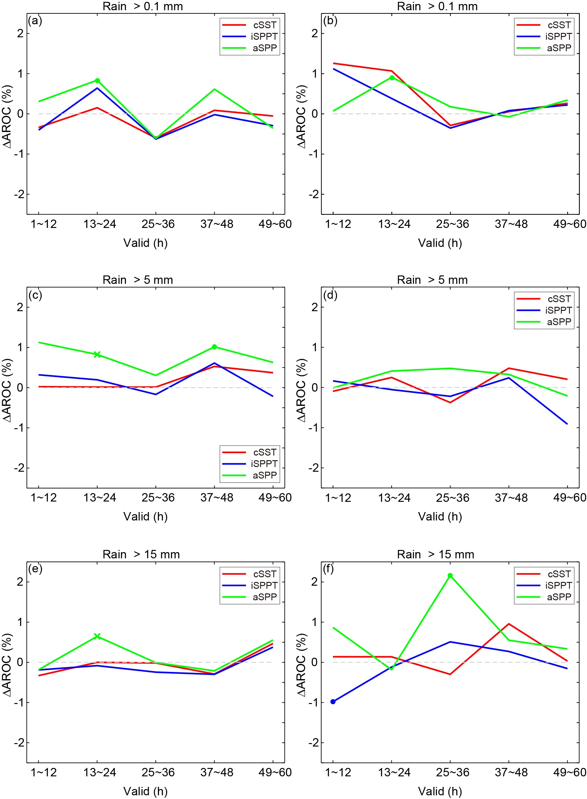
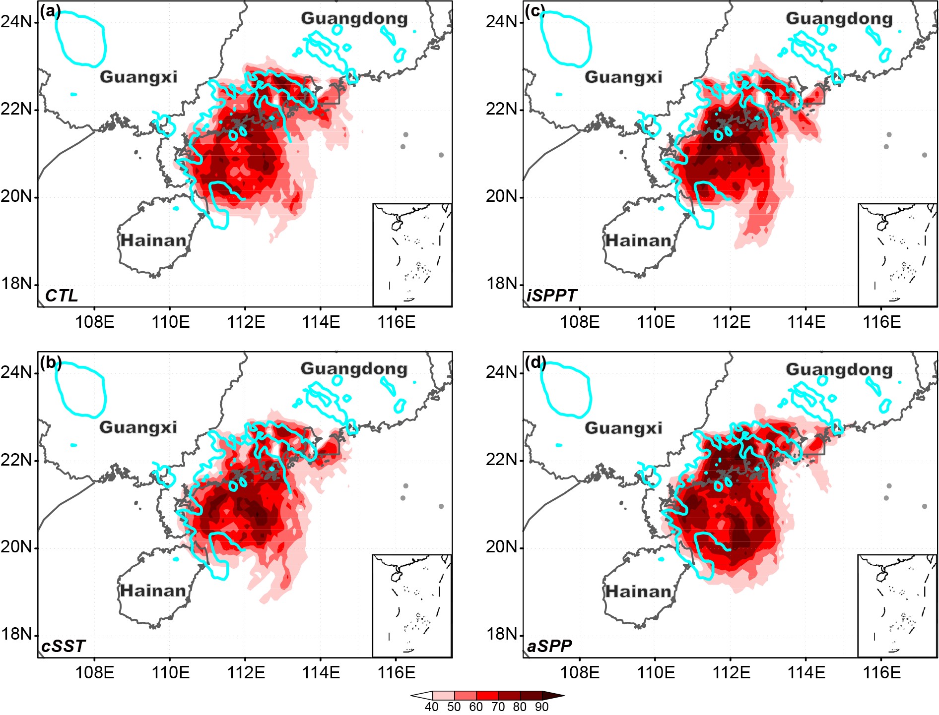
There were nearly no statistically significant AROC differences between either cSST or iSPPT and CTL for rainfall (Fig. 13). This result can be intuitively found in Figs. 14a–c. Specifically, probabilistic fields of moderate rainfall distributed similarly among CTL, cSST, and iSPPT, all of which showed lower probabilities (< 70%) around the observed moderate rainfall in the coastal area of southwestern Guangdong.
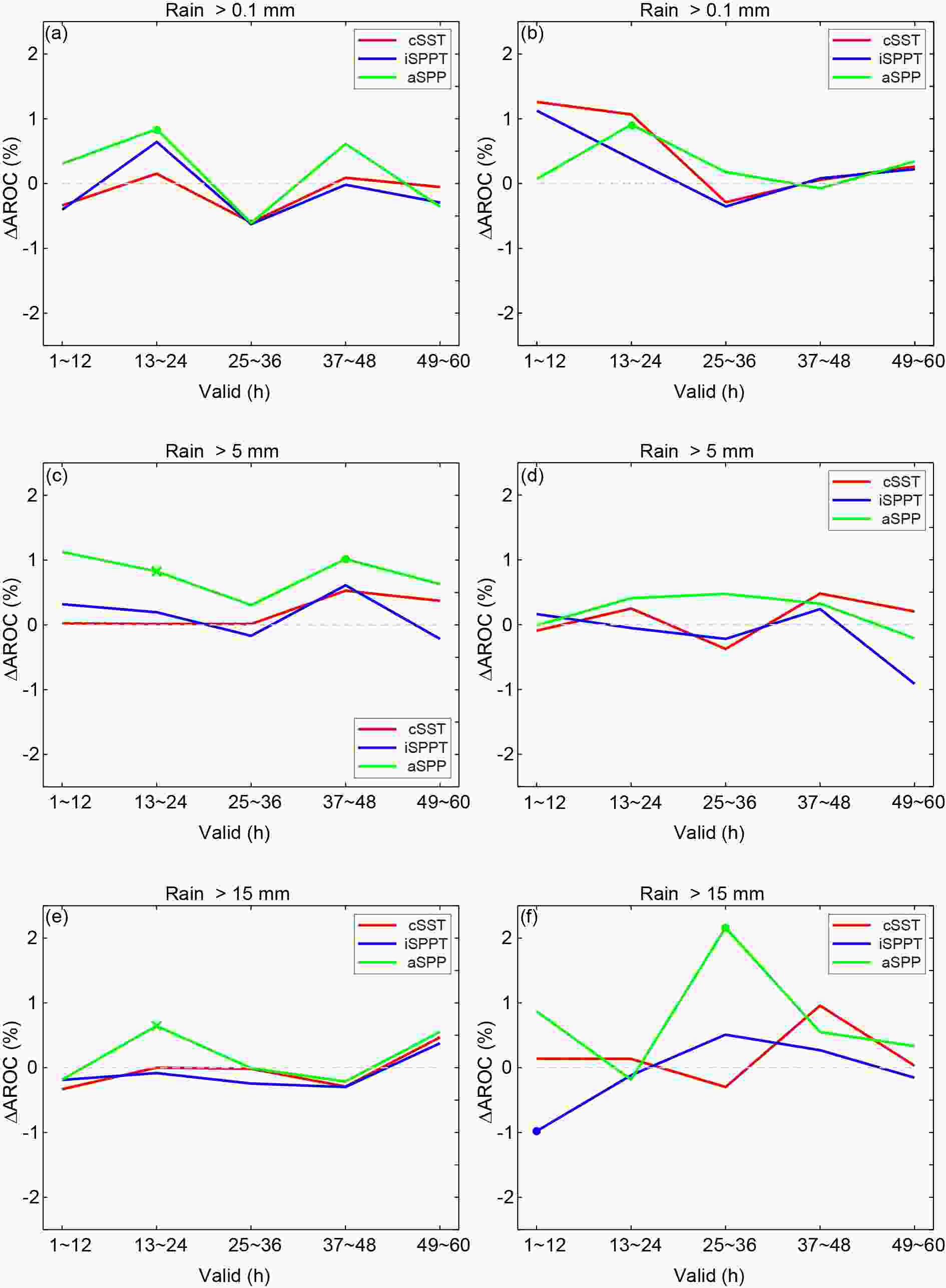
Figure 13. As in Fig. 11, but for the relative changes in AROC (ΔAROC).

Figure 14. 36-h predicted probability (%) of the 1-h accumulated precipitation exceeding 5 mm (shaded) valid at 0000 UTC 4 October 2015 for four experiments—CTL, iSPPT, cSST, and aSPP in panels (a), (b), (c), and (d), respectively. The 1-h accumulated precipitation of observations from the automatic weather stations is contoured at the 5 mm threshold in cyan lines. The range of panels is the same as the dashed rectangle shown in Fig. 1.
At most lead times, aSPP outperformed CTL in terms of AROC for rainfall of all TC cases (Fig. 13). The superiority of aSPP to CTL was comparable between intensifying and non-intensifying TCs for light rainfall (Figs. 13a, b), but was more significant for moderate rainfall of intensifying than non-intensifying TCs (Figs. 13c, d). aSPP increased occurrence frequencies of moderate rainfall over CTL more obviously at lower and higher probabilities for intensifying and non-intensifying TCs (Figs. 9e, f), respectively, leading to greater improvements in hit rates and thereby in AROC for intensifying than non-intensifying TCs (not shown). As shown in Figs. 14a, d, the observed moderate rainfall in the coastal area of southwestern Guangdong was better detected by aSPP than CTL, with probabilities above 70% in aSPP. Because the hit rates of heavy rainfall in CTL were lower in non-intensifying than intensifying TCs (not shown), greater improvements of aSPP relative to CTL in hit rates and thereby greater ΔAROC occurred in non-intensifying TCs (Figs. 13e, f).
For both surface wind and rainfall, the magnitude of ΔAROC was evidently smaller than that of ΔBSrely, indicating the smaller changes due to new implementing strategies for perturbations in discriminating ability than reliability. Such result should be expected since the discrimination is closely related to the framework and resolution of NWP models besides perturbation methods.
-
How to optimally perturb surface and model physics remains an open question for the design of high-resolution regional ensembles used for operational TC forecasting. Thus, the goal of this work was to evaluate the impacts of several new implementing strategies for SST and model physics perturbations on the TREPS forecasts of 19 landfalling TCs in 2014–16. SST perturbations were modified by replacing spatially uncorrelated random perturbations with spatially correlated ones, f-inflated SPPT was implemented based on SPPT with f inflated in regions with evident convective activity, and SPP with 14 perturbed parameters selected from the PBL, surface layer, microphysics, and cumulus convection parameterizations was added. Based on TREPS, ensemble experiments with the above three implementing strategies were carried out, respectively, and then compared to the baseline experiment run in Z18. For each ensemble experiment, 48 60-h forecasts were verified for TC cases with different intensification processes in terms of track, intensity, 10-m wind speed, and 1-h accumulated rainfall.
The performance of spatially correlated SST perturbations was generally competitive with but occasionally different from that of f-inflated SPPT. Impacts of these two perturbation methods were overall positive in the deterministic guidance of track and wind and the probabilistic guidance of wind in terms of reliability but were mixed in the forecasts of intensity and rainfall. Both perturbation methods led to greater improvements in intensity forecasting and more evident enhancements in ensemble spreads for non-intensifying than intensifying TCs. Compared with f-inflated SPPT, the spatially correlated SST perturbations were more skillful for intensity, discrimination of wind, and reliability of rainfall in intensifying TCs, but the result was opposite in non-intensifying TCs.
Adding SPP led to case-dependent impacts on TC forecasting. For intensifying TCs, adding SPP caused mixed impacts for both deterministic and probabilistic guidance. Specifically, both track and intensity forecasting were degraded but PM modest winds was significantly improved; and probabilistic forecasts of wind and rainfall were generally degraded and improved, respectively. For non-intensifying TCs, adding SPP caused more significant improvements than degradations in TC forecasting. Specifically, deterministic guidance was significantly improved in terms of track, intensity, strong winds, and moderate rainfall, while probabilistic guidance was generally improved for wind in terms of reliability and discrimination but for rainfall only in terms of discrimination.
Overall, all three new implementing strategies examined here improved forecasts more significantly for non-intensifying than intensifying TCs. This implies some benefit-limiting deficiencies of these methods in improving forecasts of intensifying TCs. To be specific, implementing the spatially correlated SST perturbations and f-inflated SPPT only around the TC may be insufficient for greatly improving the description of uncertainties related to multiscale-process interactions, which are relevant to TC RI, and thus resulted in limited and even detrimental impacts on forecasts of intensifying TCs. Future work should investigate the impacts of implementing the spatially correlated SST perturbations and f-inflated SPPT throughout the entire model domain. Moreover, the stochastic convective scheme was proposed by Tompkins and Berner (2008) to represent the forecast uncertainty due to the neglect of humidity variability on spatial scales not resolved by forecast models. Such a scheme seems to be suitable for accounting for subgrid-scale humidity variability, which is important for the trigger of convection related to RI of TCs and is planned to be tested in the future work. Because the change in surface wind field with some parameters (such as Ric and pfac) is nonlinear, the current SPP scheme used here has a potential risk of adding biases. In fact, adding SPP weakened TC intensity but strengthened surface wind outside the TC inner core. As a result, adding SPP aggravated the underestimation of intensity for intensifying TCs. It is likely that further improvements in the design of SPP achieved by properly tuning the parameter settings of the PBL parameterization could address this issue. Moreover, it is essential to elaborately select sensitive perturbed parameters which show the greatest impacts on TC forecasting to improve the SPP design. Recently, the Conditional Nonlinear Optimal Perturbation related to Parameters (CNOP-P) was applied by Wang et al. (2020) to select the most sensitive parameters that caused maximum precipitation variations for the SPP design. Such a CNOP-P based method has been confirmed to have the potential for improving forecasts of surface variables and should be applied to the SPP design in the future after properly selecting representative TC cases and metrics to calculate the cost function in CNOP-P.
In this study, all three new strategies implemented perturbations in a random way. Arguably, such implementing strategies for perturbations may not sufficiently consider the dynamically unstable growth of model errors (Qin et al., 2020). This is a possible reason why all three implementing strategies for perturbations led to less improvement in probabilistic forecasts of TC rainfall. Recently, the nonlinear forcing singular vector (NFSV) approach, which was proposed by Duan and Zhou (2013) to describe the fastest-growing of perturbations, was used to generate perturbations for model tendency (Qin et al., 2020) and SST (Yao et al., 2021). Such NFSV-type perturbations have been proven to be useful in representing forecast uncertainties related to TC intensity and will thus be considered in the future TREPS design.
Due to more observations available for analysis, the CMA best-track dataset is more accurate and complete over the offshore and land areas of China than over the open ocean (Ying et al., 2014). Thus, the verification results for TC track and intensity forecasting over the open ocean may need further confirmation based on other best-track datasets, such as the Joint Typhoon Warning Center (JTWC) dataset. Moreover, the observations of 10-m wind speed and 1-h accumulated rainfall used in the verification are from the automatic weather stations, which are largely distributed over land areas and may be damaged by severe wind and rainfall accompanied by TCs. Thus, to gain a more complete assessment for surface wind and rainfall forecasting related to TCs, other types of observations should be considered in the future work.
Finally, it needs to be mentioned that the verification scores or forecast skills of TREPS were generally comparable between intensifying and non-intensifying TCs (not shown). This indicates that forecast improvements for non-intensifying TCs are as important as those for intensifying TCs, as least for TREPS, although accurate predictions of TCs with RI remains a significant challenge. Thus, the three perturbation methods examined here, which have shown some encouraging performance in forecasting non-intensifying TCs, may provide some guidance in the ensemble design for TC forecasting.
Acknowledgements. This research was sponsored by the National Key R&D Program of China through Grant No. 2017YFC1501603, the National Natural Science Foundation of China through Grant No. 41975136 and the Guangdong Basic and Applied Basic Research Foundation through Grant No. 2019A1515011118. The author is grateful to two anonymous reviewers and the Associate Editors-in-Chief for providing constructive suggestions, which greatly improved the quality of this paper. The author thanks Xu ZHANG, Zhizhen XU, Jianfeng GU, and Zhongkuo ZHAO for helpful discussions. The support with high-performance computing from Tianhe-2 provided by the National Supercomputing Center in Guangzhou is acknowledged.
Open Access This article is licensed under a Creative Commons Attribution 4.0 International License, which permits use, sharing, adaptation, distribution and reproduction in any medium or format, as long as you give appropriate credit to the original author(s) and the source, provide a link to the Creative Commons licence, and indicate if changes were made. The images or other third party material in this article are included in the article’s Creative Commons licence, unless indicated otherwise in a credit line to the material. If material is not included in the article’s Creative Commons licence and your intended use is not permitted by statutory regulation or exceeds the permitted use, you will need to obtain permission directly from the copyright holder. To view a copy of this licence, visit
http://creativecommons.org/licenses/by/4.0/ .
| Expt. | SST perturbations | Model physics perturbations |
| CTL | Spatially uncorrelated | Combination of multi-physics and SPPT |
| cSST | Spatially correlated | As in CTL |
| iSPPT | As in CTL | Combination of multi-physics and f-inflated SPPT |
| aSPP | As in CTL | Combination of multi-physics, SPPT, and SPP |


 AAS Website
 AAS WeChat