


 DownLoad:


-
Low-level temperature inversions, characterized by an increase in temperature with height, are a common feature of major air pollution episodes. Temperature inversions in the lower atmosphere occur frequently at middle and high latitudes and serve to inhibit the mass and heat fluxes from the surface to the atmosphere, and the dilution of pollutants (Fedorovich et al., 1996; Wendisch et al., 1996; Janhäll et al., 2006; Wallace et al., 2010; Devasthale and Thomas, 2012). The presence of a temperature inversion significantly elevates the concentrations of pollutants near the ground, such as industrial and human-produced smoke, harmful gases, and particulate matter, especially when a morning surface-based temperature inversion (SBI) is present (Rendón et al., 2014; Leukauf et al., 2015). These pollutants accumulate near the ground and result in higher pollution concentrations and longer periods of poor air quality than expected (Holzworth, 1972; Malek et al., 2006; Wallace and Kanaroglou, 2009). This is detrimental to public health. In the last century, several eminent episodes of air pollution occurred around the world, resulting in thousands of deaths, and temperature inversions played a major role in these air pollution episodes (Watanabe, 1998).
As an important air pollutant, anthropogenic aerosols, especially fine particulate matter, have been correlated with morbidity and mortality, and increase the incidence of heart disease, cardiovascular disease and lung cancer (Pope et al., 1993). Aerosols also play a significant role in the earth system due to their ability to alter the radiative balance of the earth through combined direct and indirect effects (Rap et al., 2013). Vertical profiles of aerosol properties influence the transfer of shortwave radiation through the atmosphere (i.e., the aerosol direct radiative effect) and can change the calculated direct radiative forcing, as well as cloud formation and lifetime (Rehkopf et al., 1984). Significant changes in aerosol profiles are related to the presence of low-level temperature inversions (Raga and Jonas, 1995). However, which temperature inversion parameter, or parameters, affects the accumulation of aerosols near the ground and the vertical distribution of aerosols, and the relationship between these parameters and aerosols, remains uncertain and with few quantified results. This information is important for modeling the diffusion and transport of air pollutants in the lower atmosphere (Wallace et al., 2010). Little attention has been paid to the quantitative assessment of the relationship between temperature inversion parameters and aerosol concentrations near the ground, and the effect of temperature inversions on the vertical distribution of aerosols. This is in large part due to the lack of long-term aerosol and temperature profile data with consistent resolutions, and the greater difficulty in sampling aloft than from a ground-based platform (Gramsch et al., 2014). Comprehensive investigations on their relationships can greatly benefit studies of aerosol effects on weather and climate, atmospheric dynamics, and air pollution controls.
Historically, temperature inversions have been quantified using ground-based meteorological systems such as radiosondes located at widely dispersed upper-air sounding stations. Radiosonde measurements provide detailed vertical profiles of temperature, pressure, dew point, and horizontal winds, and are suited to study low-level temperature inversions (Iacobellis et al., 2009). Temperature inversion parameters, such as frequency, depth, temperature difference (dT = Ttop − Tbottom), and the temperature gradient across the inversion, have been analyzed using radiosonde data, and the main climatological characteristics of temperature inversions have been established (Bilello, 1966; Kahl, 1990; Bradley et al., 1992; Kassomenos and Koletsis, 2005; Malingowski et al., 2014). Unfortunately, conventional meteorological data suffer from some major limitations in tackling the problem of identifying temperature inversions. Around the world, World Meteorological Organization routine radiosondes are launched twice daily at 0000 and 1200 UTC. The vertical resolution was set at 50 hPa before 1970, reduced to 30 hPa from 1970–1980, and is currently around 50–80 m (Li et al., 2012). The coarse resolution is a major challenge in accurately determining the depth of temperature inversions and their fine-resolution structure. The sparse samples obtained during a day from routine radiosonde launches do not allow for an investigation of the diurnal variation in, and the frequency of, the occurrence of temperature inversions. Meanwhile, due to the high cost of operating research aircraft dedicated to collecting measurements of aerosol properties, only a few sets of in-situ vertical profile measurements have been made, and all have been made during short-term field studies on the order of weeks to months (Sheridan and Ogren, 1999; Russell and Heintzenberg, 2000; Öström and Noone, 2000). For a more accurate analysis of the characteristics of temperature inversions and their effects on aerosols in the lower atmosphere, long-term, high-quality, consistent and high spatial and temporal resolution radiosonde profiles, and aerosol and cloud data are required.
These problems can be overcome, or alleviated, considerably by using, for example, the long-term and consistent measurements of unprecedented quality made at the U.S. Department of Energy’s Atmospheric Radiation Measurement (ARM) program Southern Great Plains (SGP) site. The ARM program has provided, among other data, high-resolution radiosonde, aerosol, and radiation data, as well as atmospheric profiles from a suite of instruments for well over a decade. Radiosondes with a high vertical resolution are launched four times daily. In-situ surface aerosol number concentrations, an important air quality index, are measured by the Aerosol Observing System (AOS) at a one-minute temporal resolution. In-situ aerosol profiles (IAPs) are obtained by flying an instrumented light aircraft over the SGP site several times per week.
The purpose of this work is to characterize temperature inversions and their effects on aerosols near the ground and in the lower atmosphere, and to deduce the relationship between temperature inversion parameters and aerosol properties using 16 years of ARM data from the SGP site. Section 2 briefly describes the data and temperature inversion detection algorithm used in this study. The characteristics of temperature inversions and their seasonal variations are presented in section 3. Section 4 discusses the effects of temperature inversions on aerosols and their seasonal differences, and correlations between temperature inversion parameters and surface aerosol number concentrations. The effects of temperature inversions on the vertical distribution of aerosol optical properties are also analyzed in this section. Conclusions are given in section 5.
-
This study makes use of ARM data from the SGP site near Lamont (36.6°N, 97.5°W, 318 m) in north-central Oklahoma. The SGP site is a rural area dominated by farmland with relatively homogeneous surface of elevation ranging from 280 to 380 m above sea level. In this study, several routine ARM products such as those from the Balloon-borne Sounding System (SONDE) and the mentor-quality-controlled AOS over the period 2000–15 and IAPs from Cessna aerosol flights over the period 2000–07 were used. Väisälä radiosondes are launched four times a day (at 0530, 1130, 1730 and 2330 LST) and measure pressure, temperature, relative humidity, wind speed, and wind direction every 2 s at an average ascent rate of about 4 m s−1, resulting in a high vertical resolution of about 8 m. Based on all available profiles, the average number of temperature points is 3049 (averaged maximum height is 24 595 m) and 353 below 3 km in this work. According to the instrument’s manual, the precision for temperature and relative humidity is 0.1 K and 1%, respectively (Holdridge et al., 2011).
Aerosol data are obtained from the AOS, which is a suite of in-situ surface instruments measuring aerosol optical and cloud-forming properties at the SGP site. The primary optical measurements are aerosol scattering and absorption coefficients as a function of particle size and radiation wavelength and cloud condensation nuclei measurements as a function of percentage supersaturation. The TSI condensation nuclei counter (Model 3010) measures the in-situ total concentration of condensation particles with diameters ranging from 10 nm to 3 μm every minute. Simultaneous ground measurements of aerosol light scattering, hemispheric backscattering, and light absorption coefficients made by the three-wavelength (450, 550, and 700 nm) TSI (Model 3563) nephelometer and the Radiance Research particle soot absorption photometer are also used (Jefferson, 2011).
The IAP data were obtained by flying an instrumented light aircraft over the SGP site between April 2000 and December 2007. The total number of flights was 698. The aerosol instrument package on the aircraft was similar to the system operating at the surface (Sheridan et al., 2001). For each profile flight, the aircraft flew nine level legs from the surface to 3660 m above sea level over the SGP site. Flights were randomly made several times each week, but limited to daylight hours. The aerosol optical properties obtained for each level leg included aerosol absorption coefficient (σabs), aerosol scattering coefficient (σsca), aerosol total extinction coefficient (σext), the single-scattering albedo (SSA), the hemispheric backscatter fraction (b) at 550 nm, and the Ångström exponent (å, derived at 450 nm and 550 nm). Ambient relative humidity and temperature were measured with Väisälä sensors mounted inside a counter flow inlet on the bottom of the starboard wing. A detailed description of how the raw aerosol and ambient data from both the AOS and the IAP flights were processed to obtain these measurements is provided by Andrews et al. (2004).
-
The following temperature inversion parameters were used in this study: the height of base and top of temperature inversion layers, and their corresponding temperatures from which the temperature gradient in the temperature inversion layer was computed. An accurate determination of these parameters requires high-resolution vertical profiles of temperature (Serreze et al., 1992; Iacobellis et al., 2009) from which more realistic and complicated temperature profiles can be obtained than from routine low-resolution data. There are different ways of classifying temperature inversions (Bilello, 1966; Wolyn and McKee, 1989; Gillies et al., 2010), but the methodologies to analyze radiosonde temperature profiles still do not account for complex embedded thermal structures (Fochesatto, 2015). Because temperature inversion profiles often exhibit a complicated vertical structure, they have been classified using various methods. The algorithm used to detect temperature inversions for this study is based on the temperature inversion detection algorithm developed by Kahl (1990) and the methodology for determining multilayered temperature inversions developed by Fochesatto (2015). The depth (dz) and thermal gradient (dT/dz) of temperature inversions and embedded layers as important detection thresholds can affect the detection results, especially for shallow and weak temperature inversion. The dz of temperature inversions is greater than 40 m and that of the embedded layer is less than 40 m. The dT/dz threshold needs to be adjusted according to the depth of the temperature inversion. Fochesatto (2015) provides a detailed description of how the threshold thermal gradient is determined.
For all temperature profiles, the temperature difference across each thin layer is calculated by scanning upwards from the surface to 3000 m to find cases with temperature increasing with altitude. Temperature inversions are those with a positive dT/dz that is greater than the dT/dz threshold and with dz greater than 40 m. Within a thick temperature inversion, thin layers may be present occasionally. If these layers are very thin (i.e., < 40 m), they are considered to be embedded within the overall temperature inversion. The bottom and top of these layers are defined as the temperature inversion base and top. An SBI is defined as an inversion layer whose base is located at the surface and an elevated temperature inversion (EI) is defined as a temperature inversion layer whose base is above the surface. After temperature inversions are identified, temperature inversion parameters such as dz, dT, and dT/dz were calculated. Two profiles were taken on 17 May 2008 at 0529 LST and 15 October 2008 at 2346 LST, and were examined. The total number of temperature points below 3 km for these cases was 347 and 436, respectively. SBI top heights were located at 280 m [dT and dT/dz were 4.1°C and 1.46°C (100 m)−1, respectively] and 188 m [1.8°C and 0.96°C (100 m)−1, respectively] above the surface. Multi-layer temperature inversions were detected in the second case with the tops of the EIs located at 1100 m [dz, dT and dT/dz were 194 m, 1.7°C and 0.88°C (100 m)−1, respectively] and 2451 m [127 m, 1.0°C and 0.79°C (100 m)−1] above the surface, as shown in Fig. 1.
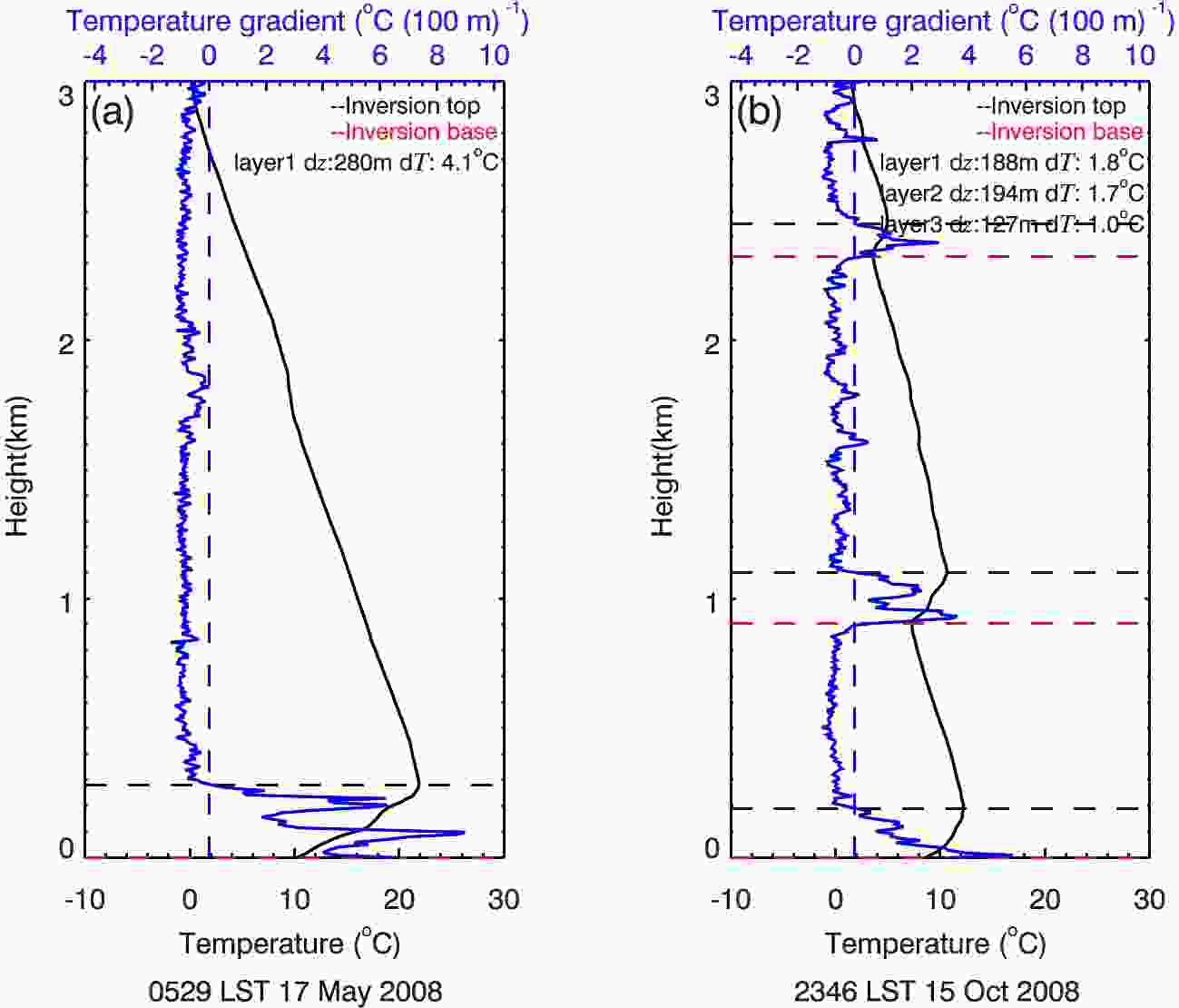
Figure 1. Vertical profiles of temperature (black lines) and dT /dz (blue lines) at (a) 0529 LST 17 May 2008 and (b) 2346 LST 15 October 2008. The dashed black and red horizontal line represents the top and base of the inversions, respectively.
-
To quantify temperature inversions, several different measures were used in this study, including the height of the base and top of temperature inversion (zbase and ztop), the depth of temperature inversion (dz), the temperature difference across the temperature inversion (dT), the temperature gradient across the temperature inversion (dT/dz), and the frequency of occurrence of temperature inversion. A total of 20 430 radiosonde profiles were analyzed over the period 2000–15, of which 99.4% (20 303 profiles) reached altitudes greater than 3 km and were used to detect temperature inversions. The temperature inversion frequencies were obtained by calculating the ratio of the number of profiles containing temperature inversion to that of all profiles. Profiles containing one, two, three, four and five temperature inversion layers accounted for 32.1%, 30.8%, 18.6%, 7.5% and 2.1% of all profiles, respectively. Multi-layer temperature inversions occurred frequently in the lower atmosphere, but few had more than five layers, so our analyses were limited to five layers. The total number of temperature inversions was 38 655 and the frequency of occurrence was 91.2%. The frequencies of occurrence of SBI and EI were 39.4% and 80.6%, respectively. For EIs, profiles containing one, two, three, four and five simultaneous EIs accounted for 35.8%, 26.0%, 13.0%, 4.9% and 0.9% of all instances of profiles containing EI, respectively. Temperature inversion frequencies at 0530, 1130, 1730 and 2330 LST are given in Fig. 2. As expected, inversions occurred at midnight far more frequently than during the day, and most frequently at dawn (99.1%).

Figure 2. Frequencies of occurrence of SBI (diagonally striped bars) and EI (gray bars) in total and at different times of the day based on data from 2000–15. Black bars represent all temperature inversions.
In terms of the time of the day, frequencies of occurrence of SBIs at 0530, 1130, 1730 and 2330 LST were 68.7%, 0.3%, 14.5% and 73.0%, respectively (Fig. 2). Most SBIs developed at night. For EIs, however, the diurnal variation was much less pronounced, with frequencies of occurrence ranging from 75.9% to 81.8%. This is partly because EIs are frequently associated with large-scale synoptic processes and their presence can vary from hours to several days. The seasonal cycles of the frequencies of occurrence for all temperature inversions, SBIs, and EIs are shown in Fig. 3. A seasonal variability is seen and is most pronounced for EIs. In general, more temperature inversions occurred in the winter, and then decreased until the summer when they reached a minimum.

Figure 3. Monthly frequencies of occurrence of all temperature inversions (black bars), SBIs (diagonally striped bars), and EIs (gray bars) based on data from 2000–15.
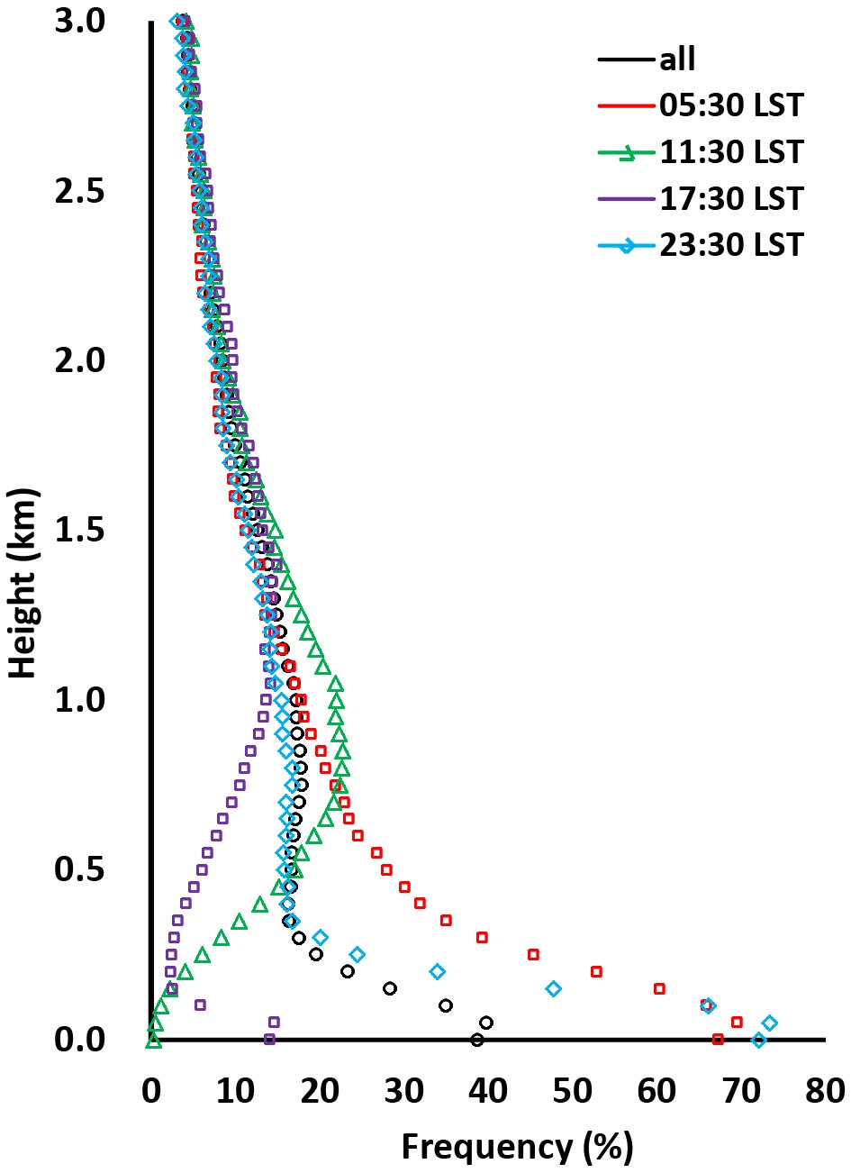
Vertical distributions of the frequencies of occurrence of temperature inversions located between the surface and 3 km are shown in Fig. 4. The diurnal variation was primarily confined to the bottommost 1 km zone. For temperature inversions at all times (black line in Fig. 4), the highest occurrence was below 200 m (39.8%) and decreased rapidly with height until it tailed off between 300 m and 400 m (16.8%). Temperature inversions occurred most frequently at midnight (2330 LST, 73.4%), followed by dawn (0530 LST, 69.5%), noon (1130 LST, 22.8%), and evening (1730 LST, 14.2%). During the day (i.e., 1130 and 1730 LST), the frequencies of occurrence generally increased with height and reached their maxima (10%–25%) between 800–1000 m. At dawn and midnight (0530 and 2330 LST), temperature inversions were more frequently near the surface than aloft. Approximately 70% of nighttime temperature inversions were below 200 m and decreased sharply with height until levelling off at 400 m. Above 1.4 km, there was little difference between the frequencies of occurrence of temperature inversions at different times of the day.
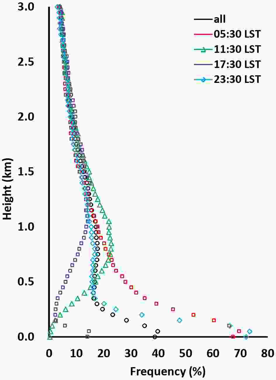
Figure 4. Vertical distributions of the frequencies of occurrence of temperature inversions located below 3 km.
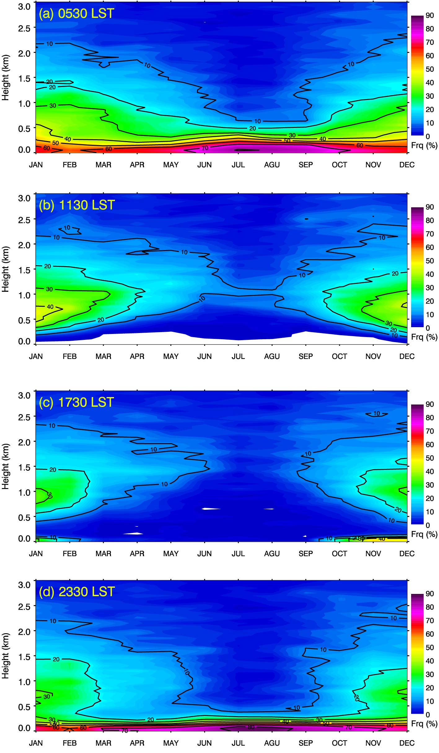
Comparing monthly vertical distributions of the frequencies of occurrence of temperature inversions for different times of the day can help understand the development and persistence of temperature inversions. Figure 5 shows the seasonal variations in the frequency of occurrence of temperature inversions at the four observation times. At dawn (0530 LST, Fig. 5a), when radiative cooling of the surface had just about reached a maximum, temperature inversions were present more than 70% of the time in late summer and early autumn, and half of them reach 300 m. By noon (Fig. 5b), solar heating had warmed the surface sufficiently enough to eliminate nearly all SBIs. These temperature inversions tended to occur above 200 m, with the highest frequency (~45%) in winter and the lowest frequency (< 5%) in summer. There were two temperature inversions in the winter evening (Fig. 5c)—one located near the ground owing to solar heating gradually weakening and radiative cooling strengthening near sunset, and the other located above 500 m (> 30%). In the summer, the SBI rarely went above 500 m (< 5%). At midnight (2330 LST, Fig. 5d), temperature inversions occurred more than 80% of the time in July, September and December. About half of these temperature inversions developed up to 200 m in July and to 300 m in December. No significant diurnal and seasonal variations in SBIs was obvious above 500 m. Temperature inversions had similar vertical distributions above 500 m at all observation times. The diurnal variation and vertical distribution of a temperature inversion is driven by changes in the surface radiation balance due to solar heating during daytime and longwave cooling at night. It is also related to synoptic large-scale conditions as well vapor pressure deficits (Mayfield and Fochesatto, 2013). Overall, near-ground temperature inversions form in the evening and gradually develop overnight, reaching their peak in frequency and thickness at dawn and dissipating before noon. Near-ground temperature inversions form earlier in the day, last longer, and are thicker in winter than in summer. Admittedly, to capture details of the temporal evolution of the temperature inversion formation in the low-level atmosphere, four observation times a day is not enough. Observation approaches using measurements with higher temporal resolutions are needed.

Figure 5. Seasonal variations in the vertical distributions of the frequencies of occurrence of temperature inversions located below 3 km at (a) 0530 LST, (b) 1130 LST, (c) 1730 LST, and (d) 2330 LST. Units: %.
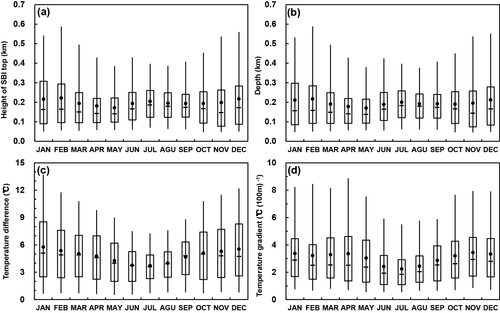
Monthly mean values of SBI parameters are shown in Fig. 6. For all SBIs, mean SBI base and top heights, dz, dT and dT/dz were 0 m, 198 m, 198 m, 4.8°C and 2.4°C (100 m)−1, respectively. The location of the temperature inversion base remained constant year-round, but the temperature inversion top height changed with season. The maximum height (216 m) occurred in February and the minimum height (169 m) in May (Fig. 6a). As such, the dz of temperature inversion had the same seasonal trend as the temperature inversion top height (Fig. 6b). The mean dT reached a minimum in the summer (3.7°C) and a maximum in the winter (5.8°C, Fig. 6c). From April to October, the mean dT/dz values of SBIs were at their lowest, reaching a minimum of 2.2°C (100 m)−1 in July. The magnitude remained constant (~3.2°C (100 m)−1 in the other months (Fig. 6d).

Figure 6. Monthly averaged SBI (a) top height, (b) depth, (c) temperature difference, and (d) temperature gradient across the temperature inversion over the 16-year period. The ends of the boxes, the ends of the bars, and the short line across each box represent the 25th and 75th percentiles, the 5th and 95th percentiles, and the median, respectively. The mean is represented by the solid circle.
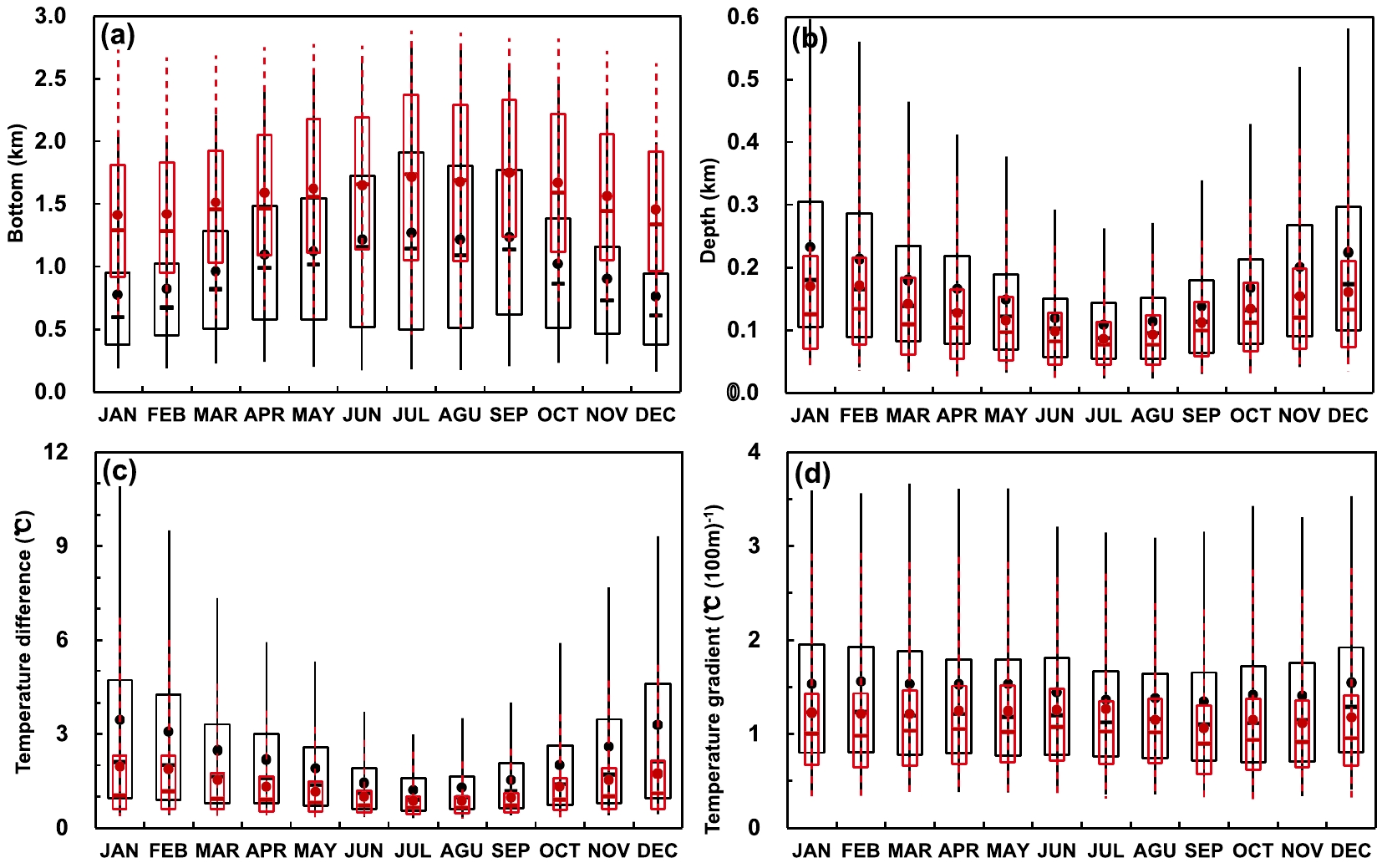
Figure 7 shows monthly mean values of first and second EI parameters. Overall, EIs are shallower than SBIs with magnitudes of dT and dT/dz that are about half the magnitudes of the dT and dT/dz of SBIs. This is because SBIs are predominantly driven by surface radiative cooling and heat advection, and both can create strong temperature inversions near the ground, while EIs are mainly synoptically controlled and are weak and shallow (Abdul-Wahab et al., 2004; Bourne et al., 2010). The mean values of the monthly averaged first EI temperature inversion base and top heights, dz, dT and dT/dz were 1039 m, 1194 m, 153 m, 2.2°C and 1.4°C (100 m)−1, respectively. For the first EI, both the base and top heights varied with season (Fig. 7a), reaching a maximum in the summertime (1273 m and 1382 m, respectively) and a minimum in the wintertime (770 m and 993 m, respectively). This is the reverse of the seasonal trend observed for SBIs. Surface heating is strong during the summer, which inhibits the development of SBIs and pushes EIs higher into the atmosphere. The temperature inversion dz and dT of EIs had the same seasonal tendencies as observed for SBIs, reaching a maximum in January (231 m and 3.4°C, respectively, Fig. 7b) and a minimum in July (108 m and 1.2°C, respectively, Fig. 7c). The dT/dz of EIs was essentially constant throughout the year (Fig. 7d). For the second EI, these parameters were 1593 m, 1703 m, 130 m, 1.3°C and 1.0°C (100 m)−1, respectively. Compared with the first EIs, the second EIs were higher, shallower and weaker. Although the second EIs had the same seasonal trends as the first EIs, the magnitudes of these trends were smaller. The average base height of the third, fourth and fifth EI was 1900 m, 2157 m and 2274 m, respectively. The average values of dz, dT and dT/dz of these EIs were similar to those of the second EI.
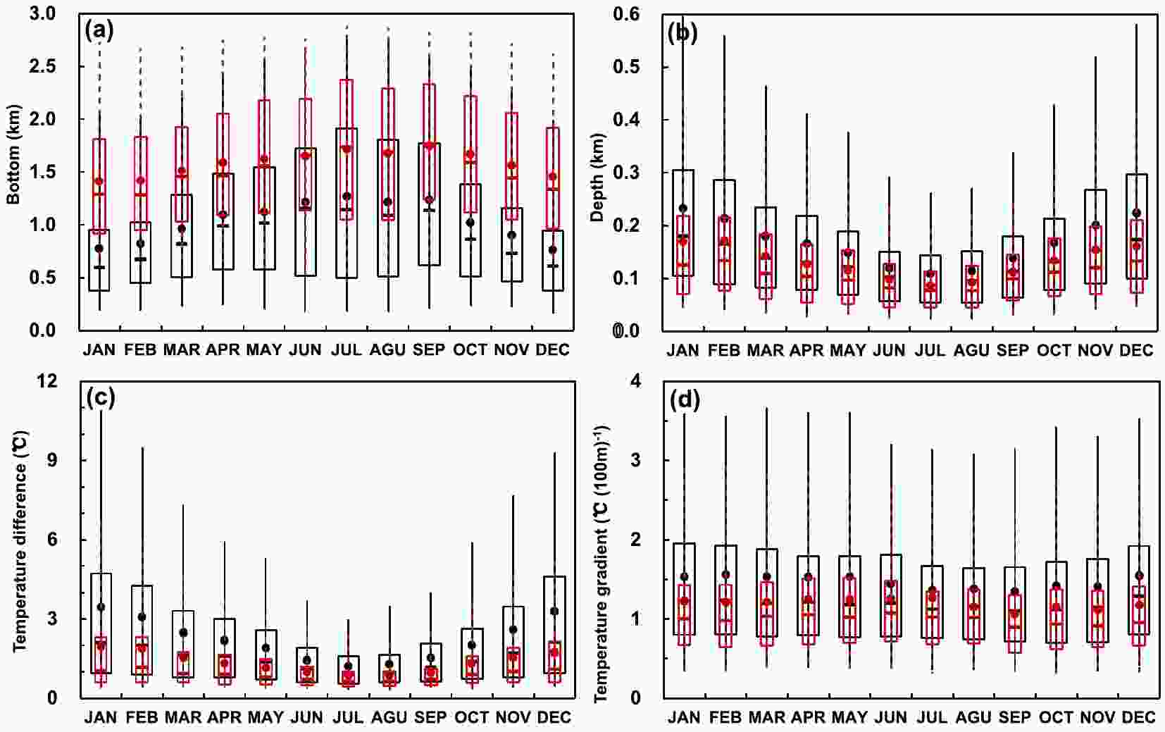
Figure 7. As in Fig. 6, but for the first EI (in black) and the second EI (in red).
-
Increases in surface-level aerosol number concentrations are associated with low-level temperature inversions. Quantifying the effect of low-level temperature inversions on aerosols is important for the study of the dispersion of pollutants (Wallace and Kanaroglou, 2009). Changes in surface aerosol number concentration when temperature inversions (both SBI and EI) were present during the 16-year period were quantified. One-hour mean surface aerosol number concentrations were obtained by averaging measurements over the 30 minutes before and after the radiosonde launch time. The effect of SBIs on aerosols during different seasons was also assessed. In addition, relationships between SBI parameters and aerosol number concentration were examined.
According to the thermal structure of a given temperature profile, the mean aerosol number concentrations of all profiles were divided into three groups, i.e., SBI, only EI, and no temperature inversion (NTI). For SBI episodes, the statically neutral residual layer usually appears above the stable boundary layer and above it is the capping inversion, which is an elevated inversion layer that separates boundary-layer air from free-atmosphere air (Stull, 1988). There is convincing evidence that residual layers have an impact on air quality in the morning (Neu et al., 1994; Fochesatto et al., 2001). To investigate the impact of the residual layer on aerosols near the ground, all SBI episodes were divided into two groups, i.e., only SBI and SBI under an EI. Tests were performed to determine whether changes in aerosol number concentration associated with the two groups were statistically significant. The methodologies used were One-way Analysis of Variance (ANOVA) and Fisher’s Least Significant Distance (LSD) test (Milionis and Davies, 2008). The null hypothesis (H0) was that no difference in mean aerosol number concentration exists due to the presence of different types of temperature inversions. H0 was tested using the F-statistic. When H0 was rejected, the one-way ANOVA could only determine that mean aerosol number concentrations among the groups were significantly different, but it did not necessarily confirm that every set of two groups was sufficiently different. The LSD test is one of multiple comparison tests that can examine this difference between groups. For the application of this test, all differences between the two groups were compared with the LSD. When the difference between two groups’ means was greater than the LSD, the two groups were significantly different at the α-significance level (i.e., 0.05).
Aerosol number concentrations near the ground and temperature inversions have obvious diurnal variations (Sheridan et al., 2001), and they interact with each other (Yu et al., 2002), so the effects of temperature inversions on aerosols are likely to have diurnal variations. To assess the diurnal variation, mean aerosol number concentrations in the presence of SBIs, EIs, SBI/EIs, and when there was no temperature inversion were compared for different times of the day. Table 1 summarizes the results of the one-way ANOVA and the LSD test for differences in the mean aerosol number concentration in the presence of a temperature inversion, an SBI, an EI or an SBI under an EI (SBI/EI), and when there was no temperature inversion. Percentage increases in aerosol number concentration due to temperature inversions are also presented. Differences in mean particle concentration at the four observation times for the four groups were statistically significant at the 95% confidence level, except at noon (the value of the F-statistic was 1.0 and almost no SBIs occurred). The LSD tests results for all observation times showed that there were significant differences (difference in means < LSD) in mean aerosol number concentration for the SBI&EI, SBI/EI&EI SBI&NTI, and SBI/EI&NTI groups, except for SBI&EI and SBI&NTI at dusk. For EI&NTI cases, however, there were no significant differences (difference in means > LSD) for all observation times. The LSD test also showed that there was significant difference for the SBI&SBI/EI group except at dawn (0530 LST). At dawn (0530 LST), mean aerosol concentrations were 49.1%, 49.4% and 4.5% higher when SBIs, SBI/EIs and EIs were present than when there were no temperature inversions, respectively. At midnight (2330 LST), these percentages were 31.3%, 36.9% and −10.0%, respectively. At dusk, the result was similar to that at midnight, whereas the magnitudes of these percentages were smaller (9.8%, 23.2% and −1.9%, respectively). At midnight and dusk, higher aerosol number concentrations appeared when an SBI under an EI was present. This result confirms that the simultaneous occurrence of the residual layers and SBI has a significant effect on the accumulation of aerosols near the ground, but this effect is weak at dawn. Slightly higher and even lower aerosol number concentrations at all observation times were seen in only the presence of an EI. This is partly because only the presences of EIs occur most frequently and are more intense during the passage of a cold front. The passage of a cold front has a strong scavenging effect on aerosols (Li et al., 2015). Aerosol number concentrations in the presence of an SBI at dusk were not significantly different to those measured with an EI or no temperature inversion present. Most SBIs formed around sunset, which were also less intense and had a weaker effect on aerosols. This result is consistent with the relationships between temperature inversion parameters and aerosol number concentration in Figs. 10b and c. At noon, when SBIs were far less frequent (1130 LST), only changes in aerosol number concentration in the presence of EIs were calculated, which amounted to a low of 7.1%.
Aerosol number concentration (cm−3) SGP 0530 LST 1130 LST 1730 LST 2330 LST SBI 4048/790 −/− 5055/158 4647/988 EI 2836/1318 4455/3860 4510/2926 3187/1204 SBI/EI 4053/2238 −/− 5668/505 4845/2365 NTI 2713/39 4157/520 4599/923 3539/78 F-statistic 153.6 1.0 16.8 156.9 LSD Test MD & LSD SBI & NTI 510 < 1333 − 554 > 455 488 < 1107 SBI & EI 147 < 1210 − 563 > 544 170 < 1459 SBI & SBI/EI 148 > 6 − 609 < 613 173 < 198 EI & NTI 525 > 123 374 > 299 257 > 89 444 > 352 EI & SBI/EI 120 < 1217 − 332 < 1158 157 < 1658 SBI/EI & NTI 583 < 1340 − 363 < 1068 543 < 1305 SBI increase 49.1% − 9.8% 31.3% EI increase 4.5% 7.1% −1.9% −10.0% SBI/EI increase 49.4% − 23.2% 36.9% Table 1. Mean aerosol number concentration (in cm−3) in the presence of an SBI, an EI, an SBI under EI, and NTI. Numbers in red are the number of profiles. DM: difference in means; LSD: Fisher’s Least Significant Distance. The significance levels of the F-test and LSD test are 5%. The LSD test results that have no significant difference are marked in bold.
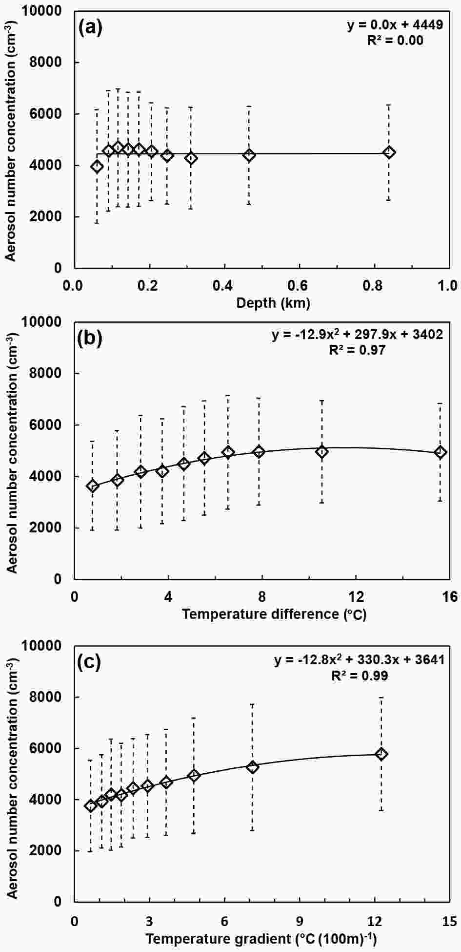
Figure 10. Aerosol number concentration as a function of (a) depth, (b) dT, and (c) dT/dz. Vertical dashed lines represent standard deviations.
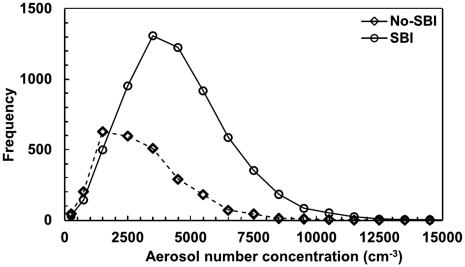
Because there were no significant differences in mean aerosol number concentration for SBI&SBI/EI and EI/NTI cases, all profiles were then divided into two categories: profiles containing an SBI, and profiles without an SBI. The effects of SBIs on aerosol number concentration were then reanalyzed for different times of the day. Table 2 shows mean aerosol number concentrations for cases with and without an SBI based on ANOVA statistics. Mean surface aerosol number concentrations increased by 43.0 %, 21.9 % and 49.2 % when SBIs were present at 0530, 1730 and 2330 LST, respectively. All the F-statistic values were greater than F0.05/2 (5.02), especially for the midnight and dawn categories. Because most profiles obtained at 0530 LST were launched before sunrise, SBI episodes at 0530 and 2330 LST were combined for the following analysis. When considering only midnight and dawn profiles, the increase in mean aerosol number concentration due to SBIs was 47.2%. The F-value was 854.9, which was much greater in magnitude than the other F-values. The distributions of aerosol number concentration frequencies at midnight and at dawn with SBIs and without SBIs present are shown in Fig. 8. All distributions seen in Fig. 8 are similar to the Fisher–Snedecor distribution, but the magnitude and location of the distribution peaks are markedly different. The aerosol number concentration peaked at 3500–4500 cm−3 when an SBI was present and reached a maximum at 1500–2500 cm−3 when there was no SBI.
SGP Aerosol number concentration (cm−3) Cases ANOVA SBI No SBI Increase % SBI No SBI F-statistic 0530 LST 4052 2833 43.0 3028 1381 450.1 1730 LST 5522 4531 21.9 663 3839 46.2 2330 LST 4786 3208 49.2 3353 1282 462.7 Midnight and dawn 4438 3014 47.2 6381 2663 854.9 Table 2. Mean aerosol number concentrations for cases with and without an SBI based on ANOVA statistics. The significance level of the F-test is 5%.

Figure 8. Distributions of aerosol number concentration frequencies during midnight and at dawn in the presence of SBIs (solid line) and when there are no temperature inversions (dashed line).
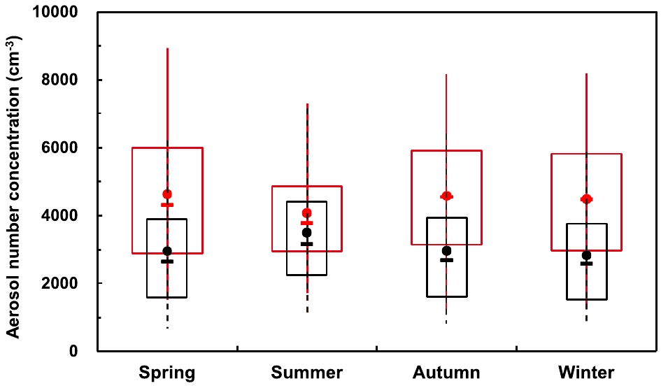
Figure 9 shows a seasonal comparison of mean aerosol number concentration for cases with and without an SBI at midnight and at dawn. The difference was smallest in the summer and larger during the other seasons. When there was no SBI, the mean particle concentration reached its peak in the summer and a minimum in the winter. The seasonal difference was smaller when no SBI was present than when an SBI was present. The presence of SBIs led to increases in mean aerosol number concentration of 56.8%, 18.1%, 55.2% and 58.4% for spring, summer, autumn and winter, respectively.
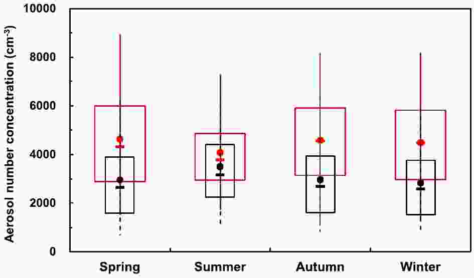
Figure 9. Seasonal comparison of mean aerosol concentrations for cases with (red) and without (black) an SBI.
The relationships between SBI parameters and aerosol number concentrations at midnight and dawn were examined quantitatively. SBI parameters (i.e., depth, dT and dT/dz) were divided into 8–10 bins, based on the magnitudes of these parameters. The mean and standard deviation of values in each bin were then calculated. Figure 10 shows aerosol number concentration as a function of the three parameters. There was almost no relationship between the depth of the SBI and aerosol number concentration (Fig. 10a), but a quadratic correlation existed between aerosol number concentration and both dT and, to a stronger degree, dT/dz, at the 95% confidence level (Figs. 10b and c). This means that the temperature difference and temperature gradient across a temperature inversion correlates fairly well with aerosol concentrations near the ground. For SBI episodes at midnight and dawn, thermally stable conditions occurred when warmer air overlay cooler, denser air. In this situation, an SBI introduces an important vertical stratification dT/dz where buoyancy is suppressed, and leads to the accumulation of aerosols near the ground. This can partly explain the relationships between SBI parameters and aerosol number concentration. The regression equations for dT and dT/dz are quadratic equations of the form: y = −12.9x2 + 297.9x + 3402.0 and y = −12.8x2 + 330.3x + 3641.0, where y is the aerosol number concentration, and x is dT or dT/dz. The surface aerosol number concentration increased with dT or dT/dz, but the mean rates of increase in aerosol number concentration decreased with dT or dT/dz. The aerosol number concentration almost never increased at dT greater than 10°C or dT/dz greater than 12°C (100 m)−1. This shows that the relationship between surface aerosol number concentration and the strength of temperature inversion is not a simple positive proportional relationship, and when temperature inversion is sufficiently strong, the effect of temperature inversion on aerosol accumulation does not increase with the increase of temperature inversion strength. These equations are helpful for the modeling of aerosol dispersion in the lower atmosphere.
The temperature gradient is the main parameter characterizing the strength of a temperature inversion and it determines low-level atmospheric stability. It is also the most relevant temperature inversion parameter associated with changes in aerosol number concentration. The combination of this strong positive relationship and the seasonal variation in dT/dz (Fig. 6d) can partly explain the seasonal differences in the effect of SBIs on aerosol number concentration at the SGP site (Fig. 9). In the summer, the temperature gradient of SBIs is at a minimum, so the mean aerosol number concentration when an SBI is present is small. For other seasons, the temperature gradient of SBIs is large with little variation, so the mean aerosol number concentration when an SBI is present is high and nearly constant with time.
-
Surface measurements of aerosol optical properties are usually used to estimate the aerosol contribution to radiative forcing, and the applicability of such calculations depends on how well surface measurements represent column properties (Andrews et al., 2004). It is important then to know the relationship between surface and aircraft measurements of aerosol optical properties. The aircraft flew 698 vertical profile flights between April 2000 and December 2007. For each profile flight, the aircraft flew over the SGP site at heights of 15, 295, 600, 905, 1210, 1515, 2125, 2735, and 3345 m. Because low-level temperature inversions with bases below 3000 m were the focus of this study, only those flight legs below this height were considered. All flight data were checked to ensure that there was valid surface data and an IAP temperature profile during the flight, and SONDE temperature profiles within one hour of the beginning or end of the flight. The total number of flights available for this study was 514. To determine how a temperature inversion (an SBI or EI) affected aerosol properties, each flight was categorized as one with an EI, an SBI, or without a temperature inversion using SONDE and IAP temperature profiles. Each flight with a temperature inversion was further categorized as one within or above the temperature inversion. The number of flights with an EI, an SBI, and without a temperature inversion was 287, 64 and 163, respectively. Mean aerosol properties measured during flight legs that were under (within) and above EIs and SBIs were compared to surface measurements.
The distribution of flight legs with respect to EIs and results from the correlation analysis for surface and vertically averaged aerosol properties for each flight leg were examined (Table 3). Relatively small samples were not analyzed because statistically significant results of small samples are usually ignored. Table 3 shows that 70% of the flights flown near 600 m (i.e., 915 m above sea level) were within an EI and that 16% of the flight legs were near 1220 m. Aerosol properties for flight legs under an EI more closely matched surface measurements than those measured above an EI. The σsca, σext and b measured during all flight legs under an EI were highly correlated with surface measurements, but poorly correlated with surface measurements when the flight leg was above an EI. Aerosol properties obtained under an EI at the two lowest flight levels correlated well with values obtained at the surface. Little correlation between surface measurements and measurements made above an EI, especially during the flight legs between 1000 and 3000 m, was seen. Results for SBIs are shown in Table 4. There was an 83% chance that flight legs below ~610 m were within an SBI. Aerosol measurements made within an SBI were highly correlated with surface measurements. The correlation at the lowest flight level was slightly better than that when an EI was present. Aerosol properties measured above an SBI and at the surface did not agree well. The correlation coefficients decreased with height and were higher in magnitude than those above an EI.
Mean height (m) Flight legs under/above EI Num σabs σsca σext SSA b å 145 285/2 0.74/− 0.96/− 0.96/− 0.71/− 0.82/− 0.55/− 295 266/21 0.71/− 0.95/− 0.94/− 0.67/− 0.82/− 0.58/− 600 200/87 0.68/0.56 0.93/0.65 0.93/0.65 0.51/0.25 0.77/0.51 0.58/0.35 915 110/177 0.59/0.53 0.90/0.44 0.90/0.45 0.29/0.26 0.67/0.11 0.34/0.26 1220 47/240 0.50/0.49 0.88/0.32 0.89/0.34 0.33/0.15 0.74/0.00 0.43/0.12 1540 12/275 −/0.31 −/0.36 −/0.37 −/0.02 −/0.00 −/0.04 2190 0/287 −/0.60 −/0.36 −/0.39 −/0.06 −/0.00 −/0.00 2780 0/287 −/0.47 −/0.36 −/0.39 −/0.00 −/0.00 −/0.00 Table 3. Correlation analysis of surface and vertically averaged aerosol properties for each flight leg over the SGP site at the 95% confidence level. The numbers of flight legs and the correlation coefficients between surface and vertically averaged aerosol properties under an EI are marked in bold.
Mean Height (m) Flight legs within/above SBI Num σabs σsca σext SSA b å 140 59/5 0.81/− 0.96/− 0.96/− 0.76/− 0.94/− 0.58/− 300 48/16 0.63/0.42 0.95/0.88 0.94/0.86 0.59/0.44 0.87/0.50 0.56/0.42 610 11/53 −/0.51 −/0.74 −/0.72 −/0.64 −/0.67 −/0.39 930 2/62 −/0.29 −/0.77 −/0.76 −/0.52 −/0.62 −/0.28 1240 0/64 −/0.31 −/0.72 −/0.70 −/0.34 −/0.39 −/0.04 1560 0/64 −/0.37 −/0.67 −/0.66 −/0.49 −/0.29 −/0.00 2200 0/64 −/0.43 −/0.49 −/0.48 −/0.36 −/0.26 −/0.00 2830 0/64 −/0.28 −/0.36 −/0.36 −/0.06 −/0.02 −/0.02 Table 4. As in Table 3, but for SBIs.
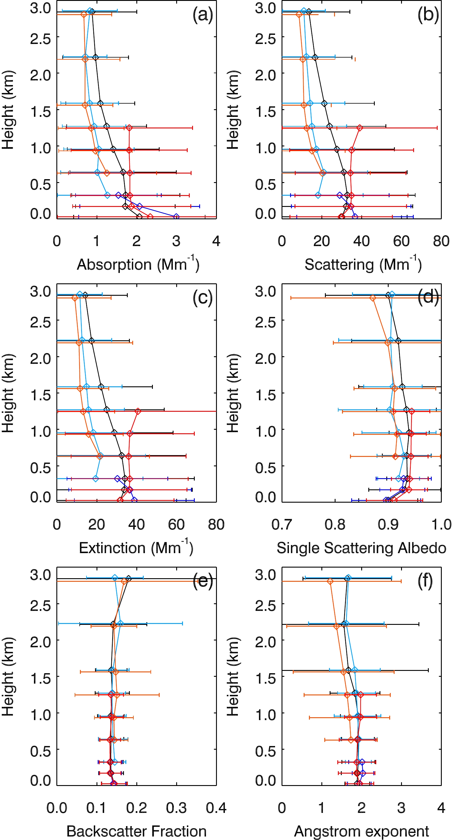
Vertical profiles of aerosol optical properties from flight legs made under different temperature inversion scenarios are shown in Fig. 11. For flights without a temperature inversion, leg-averaged σabs at the lowest flight level was greater than that measured at the surface, but σsca and σext were slightly less than the equivalent values at the surface. The leg-averaged σabs, σsca and σext tended to decrease with height from the lowest flight level upward, and became less variable with increasing height. The leg-averaged SSA, b, and å did not change much with height, had smaller differences between the different temperature inversion scenarios for flight legs below 2 km height, and were the same as at the surface except that the SSA was significantly larger. The vertical distribution of aerosol properties under an EI was different from that above an EI. The results of the one-way ANOVA and the LSD test confirmed that all aerosol optical properties measured at the surface under an EI were not significantly different to those measured without a temperature inversion present, which is consistent with the results of Table 2 for aerosol number concentration.

Figure 11. Leg-averaged (a) σabs, (b) σsca, (c) σext, (d) SSA, (e) b, and (f) å. Blue, red, and black solid lines represent SBI, EI, and NTI episodes. Dark blue (red) and light blue (red) represent aerosol properties within (under) and above SBIs (EIs). Horizontal bars represent standard deviations.
For all flight legs under an EI, leg-averaged values of aerosol optical properties appeared to be consistent, except that there was an increase in σsca and σext above 1 km. Leg-averaged σabs, σsca and σext were significantly greater than those measured when there was no temperature inversion. This difference was not seen for SSA, b and å. For flight legs above an EI, all leg-averaged values of aerosol properties except b slightly decreased with height and were significantly lower than those measured when there was no temperature inversion. The impact of EI on the vertical distribution of aerosol properties can be partly explained by the fact that the height of the EI base denotes the mixing height after sunrise (Godowitch et al., 1985) and convective mixing leads to consistent aerosol properties in a well-mixed convective boundary layer. By contrast, it is the free atmosphere above EI where aerosol particles are much lower and decrease with height. The σabs, σsca and σext measurements made at the surface during SBI episodes were significantly higher than those during EI episodes and when there was no temperature inversion. These aerosol properties within an SBI tended to decrease with height and were significantly lower than those during EI episodes near the SBI top. This result is consistent with Fig. 10. The leg-averaged values of, and trends in, σabs, σsca, σext and SSA above an SBI were similar to those above an EI. Values of b and å above an SBI were almost the same as those without a temperature inversion present. In general, the differences between aerosol properties within (under) and above temperature inversions (both EIs and SBIs) were quite large, especially for σabs, σsca and σext.
-
Knowledge of the statistical characteristics of atmospheric temperature inversions and their effects on aerosols in the lower atmosphere is important for modeling aerosol effects on weather and climate, atmospheric dynamics, and air pollution controls. A 16-year (2000–15) database of atmospheric profiles and aerosol number concentration collected at the SGP site was analyzed in terms of SBIs and EIs. This long-term and high-quality dataset was used to examine the statistical characteristics of temperature inversions and to quantify their impact on aerosols.
Temperature inversions formed at the SGP site 91.2% of the time. The frequencies of one, two, three, four and five-layered temperature inversions were 32.1%, 30.8%, 18.6%, 7.5% and 2.1%, respectively. The frequencies of SBIs and EIs were 39.4% and 80.6%, respectively. A greater number of temperature inversions formed during the night than during the day. The diurnal variation in the occurrence of EIs was smaller than that of SBIs. There was a seasonal variability in the occurrence of all temperature inversions. Diurnal and seasonal variations in temperature inversions occurred mainly below 1 km. SBIs occurred most frequently at midnight and dawn during winter, and least frequently in the summer. SBIs were generally deeper and stronger than Eis, with a mean depth of 198 m, a mean temperature difference of 4.8°C, and a mean temperature gradient of 2.4°C (100 m)−1. Multilayered EIs above first EIs had the same seasonal trends as the first EIs, but the magnitudes of seasonal trends were smaller.
Higher aerosol number concentrations appeared when an SBI was present, slight increases and even decreases in aerosol number concentration were seen in the presence of an EI, and an EI above an SBI affected the accumulation of aerosols near the ground at midnight and dusk, but had little effect on aerosol number concentration at dawn. The increase in mean aerosol number concentration in terms of percentage due to the presence of SBIs was 43.0%, 21.9% and 49.2% at 0530, 1730 and 2330 LST, respectively. At the SGP site, there was almost no correlation between SBI depth and surface aerosol number concentration. The aerosol number concentration correlated well with temperature difference or gradient across the temperature inversion layer. Two quadratic regression equations were derived based on this relationship. Temperature differences and temperature gradients across SBIs correlated fairly well with aerosol number concentrations, especially for temperature gradients. However, the mean rates of increase in aerosol number concentration decreased with temperature differences and temperature gradients across SBIs, and there was no positive correlation between aerosol number concentration and temperature inversion strength when temperature inversion was sufficiently strong. A detailed analysis of aerosol vertical profiles in conjunction with temperature inversions detected revealed that aerosol properties within (under) and above temperature inversions were different. Surface measurements were representative of the air within, but not above, SBIs and EIs. The presence of SBIs and EIs led to significant increases in leg-averaged aerosol properties within (under) the temperature inversions, and apparent decreases above the temperature inversions, especially for σabs, σsca and σext.
To capture details of the temporal evolution of the temperature inversions and their effects on aerosols in the low-level atmosphere, only one site and four observation times a day are not enough. Further investigations will be conducted with multi-site observation approaches using measurements with higher temporal resolutions.
Acknowledgments. The data used in this work were made available by the ARM Program sponsored by the U.S. Department of Energy. We thank Maureen Cribb and Ntwali Didier for their suggestions. This work was supported by the Strategic Priority Research Program of the Chinese Academy of Sciences (Grant No. XDA17010101), the National Natural Science Foundation of China (Grant Nos. 41305011, 41775033, 41575033 and 41675034), the China Postdoctoral Science Foundation (Grant No. 2014M550797), and the National Key R&D Program of China (Grant No. 2017YFA0603504).
| Aerosol number concentration (cm−3) | ||||
| SGP | 0530 LST | 1130 LST | 1730 LST | 2330 LST |
| SBI | 4048/790 | −/− | 5055/158 | 4647/988 |
| EI | 2836/1318 | 4455/3860 | 4510/2926 | 3187/1204 |
| SBI/EI | 4053/2238 | −/− | 5668/505 | 4845/2365 |
| NTI | 2713/39 | 4157/520 | 4599/923 | 3539/78 |
| F-statistic | 153.6 | 1.0 | 16.8 | 156.9 |
| LSD Test | MD & LSD | |||
| SBI & NTI | 510 < 1333 | − | 554 > 455 | 488 < 1107 |
| SBI & EI | 147 < 1210 | − | 563 > 544 | 170 < 1459 |
| SBI & SBI/EI | 148 > 6 | − | 609 < 613 | 173 < 198 |
| EI & NTI | 525 > 123 | 374 > 299 | 257 > 89 | 444 > 352 |
| EI & SBI/EI | 120 < 1217 | − | 332 < 1158 | 157 < 1658 |
| SBI/EI & NTI | 583 < 1340 | − | 363 < 1068 | 543 < 1305 |
| SBI increase | 49.1% | − | 9.8% | 31.3% |
| EI increase | 4.5% | 7.1% | −1.9% | −10.0% |
| SBI/EI increase | 49.4% | − | 23.2% | 36.9% |
 AAS Website
 AAS WeChat