Modeling Arctic Boundary Layer Cloud Streets at Grey-zone Resolutions

Cloud modeling remains a challenge in today’s numerical climate and weather models, in large part because cloud phenomena operate on a wide range of scales, from individual cloud particles (micrometers) to synoptic weather systems (hundreds to thousands of kilometers) (Hong and Dudhia, 2012; Lebo et al., 2017). In general, atmospheric motions that form clouds cannot be resolved by global or regional models and therefore must be parameterized by cumulus and boundary layer schemes. To better simulate and represent clouds in models, high-resolution grids are more and more often used to better resolve motions associated with cloud phenomena. For instance, major operational global numerical weather prediction models are moving toward cloud-resolving scales, including the NCEP Global Forecast System (Tallapragada, 2017) and the ECMWF Integrated Forecasting System (Buizza et al., 2018; Zhang et al., 2019).

Several studies have investigated the advantages of using high-resolution models for cloud modeling. The sensitivities of cloud dynamics and thermodynamics to decreasing horizontal and vertical grid lengths have been explored at both the mesoscale and large-eddy scale. Clouds have marked different vertical redistribution characteristics as a result of changes in vertical resolution (Lane et al., 2000; Roeckner et al., 2006; Byrkjedal et al., 2008). Cheng et al. (2010) investigated the effects of varying horizontal grid spacing in a large-eddy simulation (LES) and found that different cloud properties (e.g., cloud size, fraction, and amount) were sensitive to horizontal grid spacing, vertical grid spacing, or both. Stevens et al. (2002) found that not only cloud types varied with changes in model resolution, but the entrainment and vertical fluxes of heat, moisture, and momentum were sensitive to model resolution as well. Khairoutdinov and Randall (2003) showed that the vertical velocity, which represents the resolved vertical motions, and the updraft and downdraft mass fluxes were sensitive to the grid length. With different resolved conditions, clouds and atmospheric variables affected by clouds have different characteristics. Field et al. (2017) investigated a cold air outbreak that showed that with decreasing horizontal grid spacing (16 km to 1 km), the simulated long- and shortwave irradiances became closer to satellite observed values for cumulus clouds, but these irradiances differed more from the observed values for stratocumulus clouds. Gao et al. (2017) demonstrated an improvement in the spatial distributions and diurnal variability of clouds and precipitation systems with smaller grid lengths (from 36 km to 4 km). These earlier studies showed great sensitivity in simulation outcomes by tuning model resolutions.

Many studies have focused on clouds in the Arctic because of the generally poor representation of Arctic clouds in models (e.g., Inoue et al., 2006; Tjernström et al., 2008; Wyser et al., 2008; de Boer et al., 2014). The formation and dissipation of Arctic clouds within the boundary layer are strongly affected by turbulence, so previous studies have resorted to cloud-resolving models or LES (e.g., Jiang et al., 2000; Inoue et al., 2005; Luo et al., 2008; Fan et al., 2009; Klein et al., 2009; Solomon et al., 2014; Savre and Ekman, 2015). LES is a numerical modeling approach that explicitly resolves energy-containing turbulent motions responsible for most of the turbulent energy transport within the boundary layer, and is typically applied to features with scales from 1 km down to 100 m. Gryschka and Raasch (2005) showed that the cloud structure of a cold air outbreak was captured via applying LES with a horizontal grid length of 50 m. Although previous studies have investigated the capability of cloud-resolving models and LES to simulate Arctic clouds, the transition of the boundary layer environment and cloud structures within the grey zone and sub-kilometer scales in numerical weather models has not been systematically addressed. Grey zone, or “terra incognita” after Wyngaard (2004), here means that the spatial filter scale and the length scale of the energy containing features to be simulated are comparable in magnitude, and neither mesoscale planetary boundary layer (PBL) turbulence parameterizations nor LES closure assumptions are strictly valid to simulate turbulent features at this scale. In the traditional (and more appropriate) frameworks, the spatial filter scale in large eddy simulation is much smaller than (approximately a tenth of) the feature scale and resolves the large eddies; and for the mesoscale, the spatial filter scale is much larger than (approximately ten times) the feature scale and parameterizes all of the turbulence.

In this study, we investigated a case of roll clouds in the Arctic and their boundary layer dynamics using a model with resolutions ranging from convection-parameterized (> 10 km), down to cloud-resolving (a few kilometers to 1 km), and finally to large-eddy-permitting (LEP) (1 km down to 100 m) grid spacing. The LEP concept was introduced in Green and Zhang (2015) to refer to modeling scales that begin to resolve large energy-containing turbulent eddies but may not be sufficient to be true LES, which typically has a grid spacing smaller than 100 m. Thus, LEP denotes use of LES turbulence closure despite the fact that the large eddies are not well resolved. We focused on roll clouds because they are common features in the Arctic atmospheric boundary layer and their typical scales range from hundreds of meters to a few kilometers for a single roll, and tens to hundreds of kilometers for the whole cloud deck (Kuettner, 1959, 1971; Young et al., 2002). Several previous studies used LES or LEP simulations to examine cloud streets and their associated turbulent kinetic energy budgets, fluxes of momentum, and microphysical properties (Moeng and Sullivan, 1994; Glendening, 1996; Rao and Agee, 1996; Khanna and Brasseur, 1998; Harrington and Olsson, 2001). Because the dynamical interactions involved in rolls are between the mesoscale and large-eddy scale, we performed a series of sensitivity tests with varying horizontal resolution and with or without LEP to better understand how model resolution affects the formation of Arctic boundary layer roll clouds.

The aim of the study was to develop a model-based picture of roll clouds at horizontal spatial resolutions across the mesoscale and grey zone to the near large-eddy scale and apply this knowledge to the cloud features observed in our case. In addition to examining the characteristics of the Arctic roll clouds that occurred during the case study, we also investigated the mesoscale environment, horizontal and vertical cloud structures, boundary layer stability, and buoyancy and shear as sources of turbulence production, all of which were subsequently used to interpret the observed roll-cloud case. To support the interpretation of the mesoscale and LEP scale modeling studies with associated sensitivity tests, we analyzed a diverse set of observations, including satellite radiances, balloon-borne soundings, surface observations, and a reanalysis dataset.

The case study period consisted of small-scale roll clouds embedded in a much larger-scale environment that supported their formation.

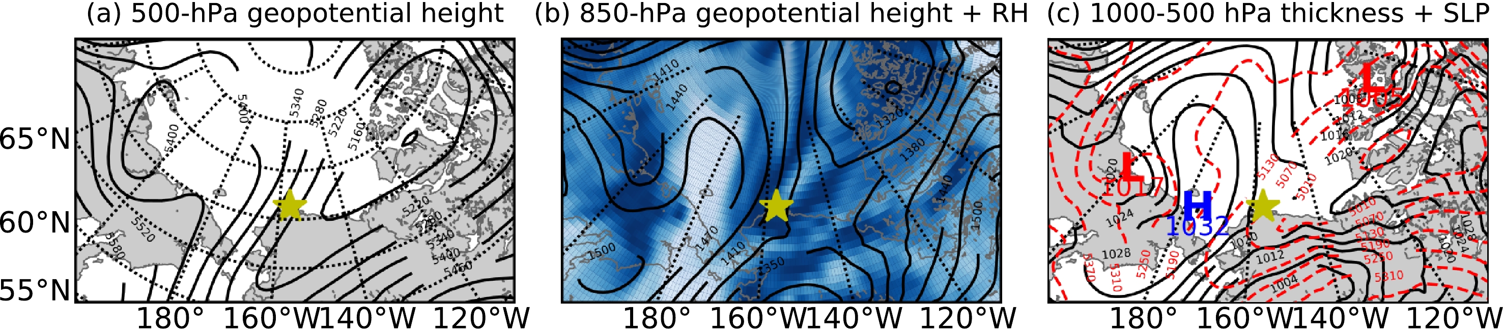
This study focused on a case of Arctic roll clouds or cloud streets that occurred on 2 May 2013. The atmospheric conditions for this case were analyzed with ERA-Interim data with a spatial grid of 0.75° latitude by 0.75° longitude. At 0000 UTC on 2 May 2013 there was a dominant high pressure system over the Chukchi Peninsula and Chukchi Sea, along with a low pressure system at 500 hPa over the Canadian Arctic Archipelago with a trough that extended toward the southwest, just southeast of Utqiaġvik (Fig. 1). The prevailing wind direction at Utqiaġvik was from the northeast, advecting 850-hPa moisture into the Utqiaġvik region (Fig. 1b). As Fig. 1c shows, the thickness between 500 hPa and 1000 hPa decreased from the northwest to southeast of the domain. A warm air mass was advected into the region from the north near the surface, associated with a surface warm front in the vicinity of Utqiaġvik at this time.

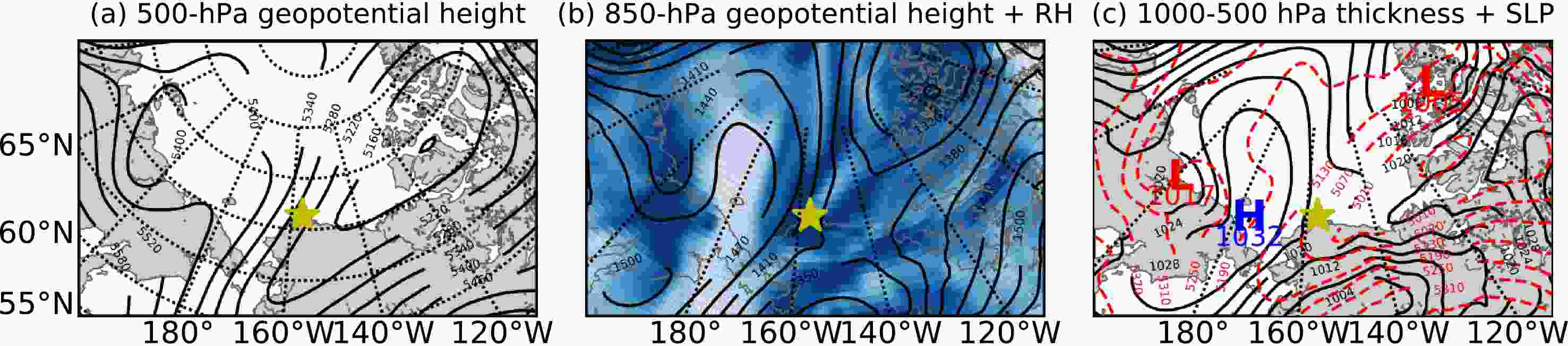
Figure 1.  ERA-Interim data at 0000 UTC 2 May 2013: (a) 500-hPa geopotential height (units: m, black contours), (b) 850-hPa geopotential height (units: m, black contours) and relative humidity (units: %, blue shading, with darker blues indicating higher relative humidity), and (c) 1000–500-hPa thickness (units: m, red dashed contours) and sea level pressure (units: hPa, black contours). The yellow stars indicate the location of Utqiaġvik and the red Ls and blue H indicate the locations of the low and high pressure centers.

The Moderate Resolution Imaging Spectroradiometer (MODIS) onboard the NASA Terra and Aqua satellites frequently passed over Utqiaġvik and its vicinity during the case study period. MODIS band 1 (band-center wavelength of 0.65 μm) visible imagery collected at 0015 UTC 2 May and 0445 UTC 2 May is presented in Figs. 2a and b. At this time, the Beaufort and Chukchi seas were covered by sea ice but with leads evident in the sea ice throughout the region, and the North Slope of the Alaskan land surface was covered by snow.

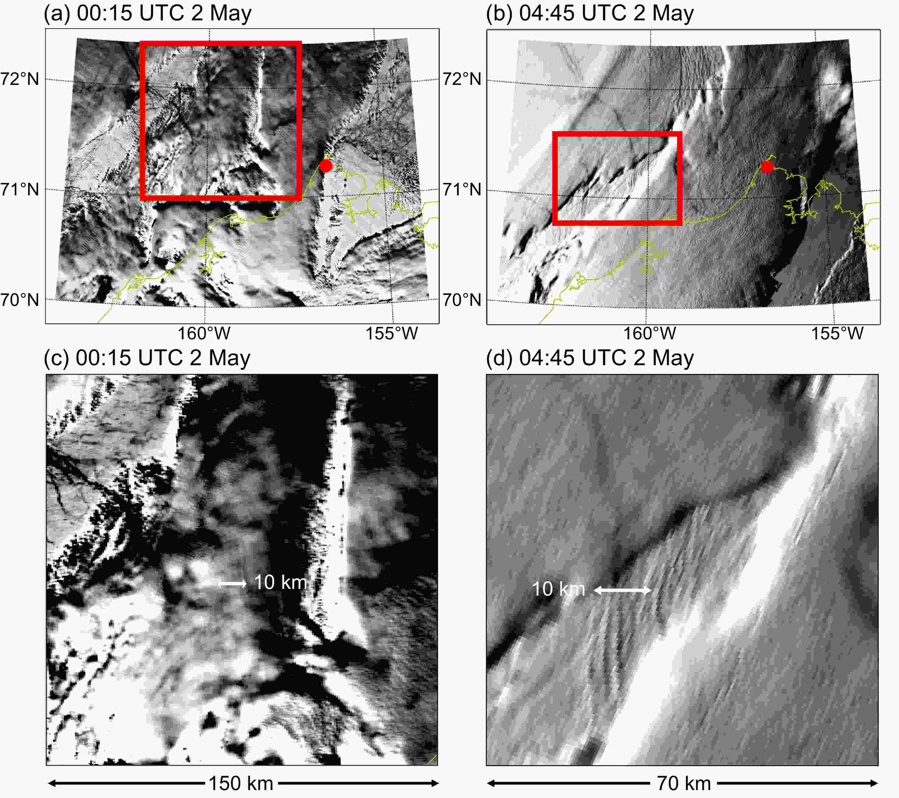
Figure 2.  Observed radiances from Terra MODIS band 1 in the vicinity of Utqiaġvik at (a) 0015 UTC 2 May and (b) 0445 UTC 2 May. (c, d) Radiances for the red boxes in (a, b), respectively. The red dots denote the location of Utqiaġvik.

Figures 2a and b reveal that many of the cloud layers to the west and south of Utqiaġvik either contained evidence of waves or were cloud streets in their entirety from 0015 UTC 2 May to 0445 UTC 2 May 2013. At 0015 UTC 2 May, Utqiaġvik was at the eastern edge of the frontal cloud band with cloud streets occurring to the west of the frontal cloud band (Fig. 2a, red box). At 0445 UTC the frontal cloud band had broadened, filled in, and moved to the east, covering Utqiaġvik in a deck of clouds. At this time, lower altitude roll clouds were present to the west of Utqiaġvik under a gap in the cloud deck (Fig. 2b, red box). To estimate the wavelengths of the cloud streets to the west of Utqiaġvik, we used Figs. 2c and d, which show detailed features of the cloud streets within the red boxes in Figs. 2a and b. We obtained a wavelength of approximately 2.5–2.8 km for the cloud streets to the west of Utqiaġvik.

We used a numerical weather model to investigate the formation mechanisms of the roll clouds identified in Figs. 2c and d along with the influence of different model spatial resolutions on the model results. The numerical weather model employed in this study was the Weather Research and Forecasting (WRF) model (Skamarock et al., 2008), version 3.6.1. The model spatial resolutions in our experiments ranged from the mesoscale to LEP scale in order to capture both the large-scale environment and cloud-resolving scales of the roll clouds evident on 2 May 2013.

We implemented six one-way nested domains over the northern part of Alaska, the Beaufort Sea, and the Chukchi Sea starting from a horizontal grid spacing of 27 km on the outer domain and working in domain ratios of 3:1 down to an inner domain with 111-m grid spacing (Fig. 3). Domains D01 through D06 had spatial grid spacing of 27 km, 9 km, 3 km, 1 km, 0.333 km, and 0.111 km. By using one-way nested domains, no information from the inner domains was passed back to the parent domains and the results from each domain illustrate what was produced at that grid spacing. We used terrain-following vertical levels with 33-m grid spacing within the boundary layer. The vertical grid spacing increased with increasing altitude up to the top of the model at 50 hPa, where the grid spacing was about 23.6 hPa. Overall, there were a total of 130 vertical layers.

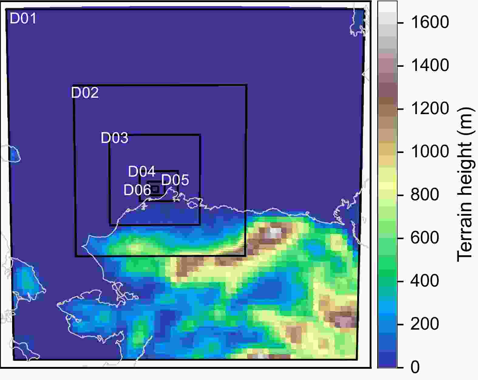
Figure 3.  WRF model domain for the mesoscale and large-eddy simulations. Shading shows the terrain height.

The five outer domains D01–D05 ran as mesoscale domains while the inner domain D06 ran as an LEP domain. The physical parameterizations used in the simulations were as follows. The Grell 3D scheme was chosen for the cumulus parameterization for domains D01 and D02, and the Morrison double-moment scheme was chosen for the microphysics in all domains. The Noah land surface model and NCAR Community Atmospheric Model radiation schemes were used for land surface and atmospheric radiation processes, respectively.

For a mesoscale model the covariance terms (e.g., $\overline {u_i'u_j'} $) that represent the effects of turbulence on the mean motion in the momentum equations are unknowns and must be parameterized by a planetary boundary layer (PBL) scheme. In LEP, a subgrid-scale (SGS) parameterization is still used to represent the processes of the turbulence smaller than the grid scale. To resolve most of the large energy-containing turbulence, the grid spacing must be much smaller than the large energy-containing eddies (e.g., Wyngaard, 2004).

For our case, the Mellor–Yamada–Janjic scheme, which is a turbulent kinetic energy based PBL scheme, was used for domains D01 through D05. We designed domain D06 to resolve large eddies, so we turned off the PBL scheme within this inner domain. Subgrid eddy diffusion within this LEP domain was based on the three-dimensional LES turbulent kinetic energy closure of Deardorff (1980) (Table 1).

To examine if the horizontal resolution of domain D06 was necessary for resolving the observed roll clouds, we ran another experiment with the four outer domains (D01–D04) using the same configuration as the experiment mentioned above but with the fifth domain D05 as an LEP domain, with the same settings as the LEP domain D06. Table 1 shows that domain D05 was run both as a mesoscale domain with a PBL parameterization, D05 (PBL), and also as an LEP domain, D05 (LEP).

The initial and boundary conditions used in the simulations were a combination of water vapor mixing ratios from ERA-Interim reanalysis and the remaining meteorological variables from the NCEP Global Forecast System final analysis, because sensitivity tests with this combination led to results that best matched observations of the horizontal wind fields and vertical moisture distributions. The data prescribed sea ice across the domain, except for the southern part of the Chukchi Sea, and snow covered the model land surfaces. All of the domains in the simulations started simultaneously at 1800 UTC 1 May 2013 and ran for six hours to 0000 UTC 2 May 2013.

For assessing general WRF model performance we compared the simulated boundary layer conditions during this period at Utqiaġvik with balloon-borne sounding data collected by the U.S. National Weather Service in Utqiaġvik, Alaska, at 2300 UTC 1 May 2013. At this time, the observed boundary layer was neutral below 400 m with capping inversions just above 400 m and at 1500 m with weaker stability in between from 600–1500 m (Fig. 4a, black line). Below 250 m the sounding data had been flagged as questionable so were not used in our analysis. The near-surface 2-m temperature observations (Fig. 4a, cross markers) were from the Department of Energy (DOE) Atmospheric Radiation Measurement (ARM) Climate Research Facility surface meteorology systems. Although we did not have direct observations of the near-surface conditions below 250 m due to uncertainty in data quality, near-surface observations indicate that this region was stably stratified. Dewpoint temperatures were closest to air temperatures near 400 m and 1500 m. High Spectral Resolution Lidar backscatter and Ka-band ARM zenith radar reflectivity at this time indicated clouds at 1500 m associated with the frontal system as well as cloud streets between 400–600 m (Oue et al., 2016). Vertical shear in the horizontal wind speed occurred from near the surface to 300 m of altitude and directional wind shear from 300–600 m of altitude (Fig. 4b).

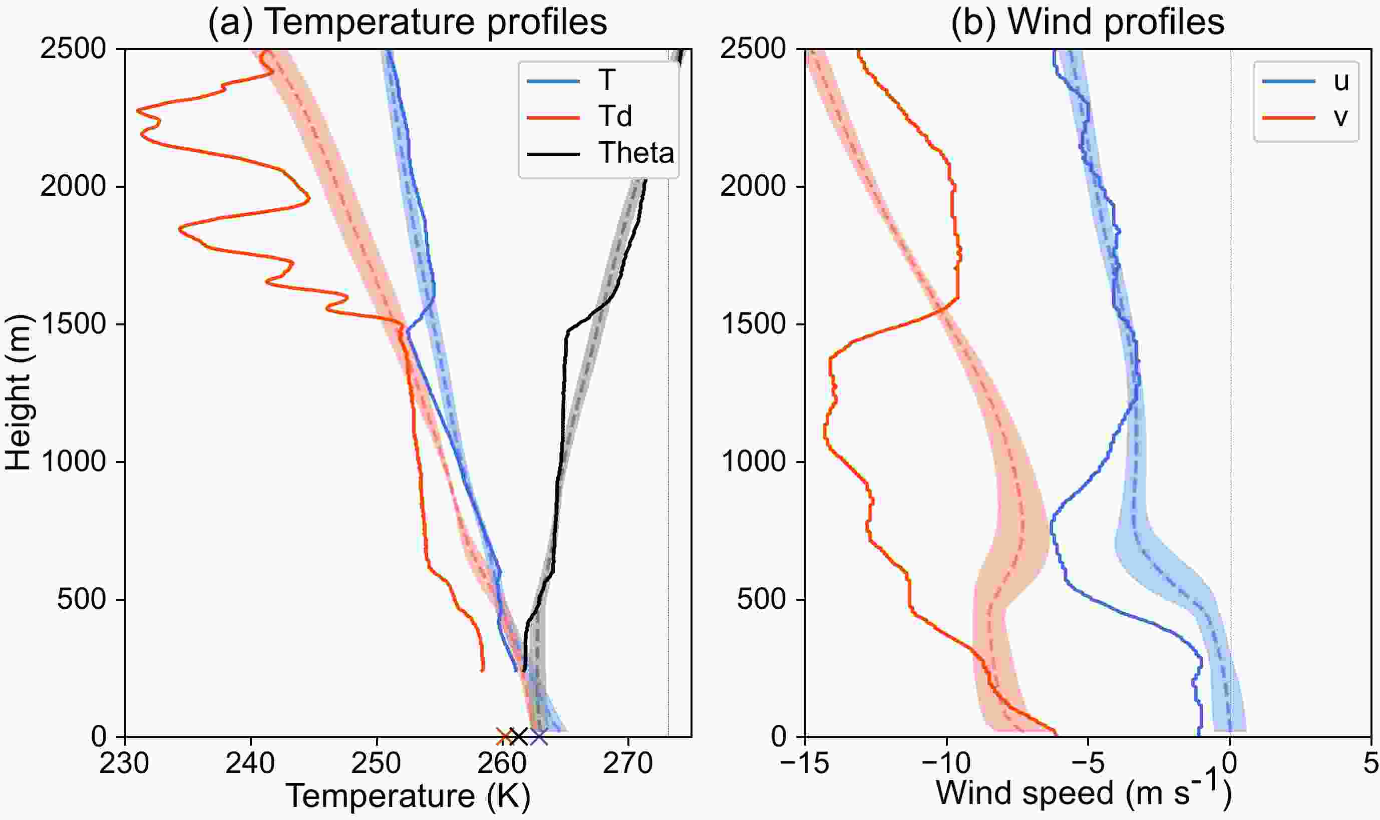
Figure 4.  Vertical profiles of (a) potential temperature (black line), temperature (blue line), and dewpoint temperature (red line), and (b) u-wind (blue line) and v-wind (red line) from the balloon-borne sounding launched at 2300 UTC 1 May at Utqiaġvik, together with WRF output of the same variables at 2200 UTC 1 May averaged over a 3° × 1° box centered on Utqiaġvik. The shading around the WRF averaged profiles (dashed lines) represents ±1 standard deviation. The three cross markers (×) in (a) indicate the 2-m temperature measurements from the ARM surface meteorology systems.

Simulated profiles for Utqiaġvik were obtained from averages of domain D04 output over a 3° longitude × 1° latitude (~110 km × 110 km) box centered on Utqiaġvik at 2200 UTC. The box was limited to domain D04 because the sounding represented the front and rolls environment near Utqiaġvik, and the 1-km grid spacing domain D04 was the finest domain covering the clouds over Utqiaġvik (Figs. 1b and 3). The simulated potential temperature shows a neutral environment below 500 m and the model captured the temperature inversion at about 600 m height (Fig. 4a, black and blue shading). The overlap of temperature and dewpoint temperature between 250 m and 600 m indicates a potential location of the simulated cloud layer. The model produced weaker u-component wind shear between 300–600 m and weaker v-component wind shear below 1500 m than in the observations (Fig. 4b). Moreover, the simulations failed to reproduce the inversion and frontal clouds observed at 1500 m. The observed frontal system was simulated to the north of Utqiaġvik, thereby missing the capping inversion at 1500 m. In this study we focused on the low-level roll clouds underneath the frontal clouds. Thus, we analyzed the dynamics and thermodynamics related to only these rolls.

To understand how the simulated boundary layer conditions changed with different grid spacing, we examined the vertical profiles of virtual potential temperature, water vapor mixing ratio, and winds from the different domains (Fig. 5). The simulated mean vertical profiles were averaged over a 0.6° longitude × 0.2° latitude (~22 km × 22 km) box centered on the middle of the LEP domain D06 for meteorological fields from domains D03 to D06, inclusive. The size of this box covered most of the area of domain D06, but avoided impacts from the lateral boundaries. At 2200 UTC, the virtual potential temperatures from the PBL domains D03, D04, and D05 first decreased with increasing height above the surface up to about 200 m; from 200 m to 500 m the virtual potential temperatures increased with increasing resolution, thereby changing from a slight negative slope (PBL D03) to a positive slope (PBL D05). At this time, the surface skin temperatures in all of the domains were higher than for the lowest model level, which indicates a buoyant environment near the surface. Both LEP domains D05 and D06 produced virtual potential temperatures that increased monotonically with height from the near-surface to 500 m (Fig. 5a). The difference in near-surface virtual potential temperature between PBL D05 and LEP D05 was approximately 1° K. The virtual potential temperature inversion from 500 m to 700 m increased with coarser horizontal grid spacing. In summary, in the LEP simulations the boundary layer was more near-neutral, as judged by the fact that the average model virtual potential temperature (i.e., θ_v) profile showed a slight increase with height. In addition, the temperature profiles were more sensitive to switching from the PBL to the LEP domain than decreasing model grid spacing.

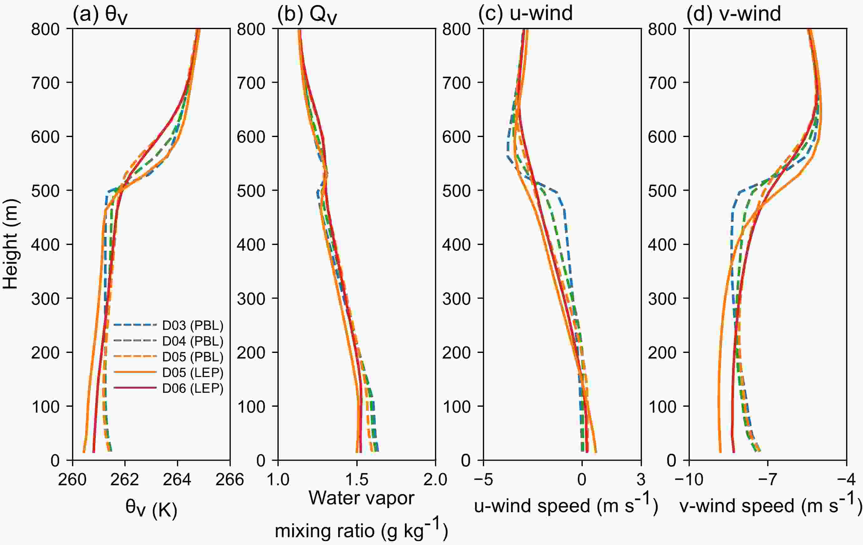
Figure 5.  Vertical profiles of (a) virtual potential temperature, (b) water vapor mixing ratio, (c) u-wind, and (d) v-wind at 2200 UTC 1 May within a 0.6° × 0.2° box centered on the middle of domain D06 but from domains PBL D03 (blue dashed lines), PBL D04 (green dashed lines), PBL D05 (orange dashed lines), LEP D05 (orange solid lines), and LEP D06 (red solid lines).

The vertical distribution of water vapor mixing ratio was also affected by the model resolution (Fig. 5b). Near the surface, the difference of water vapor mixing ratios decreased monotonically with decreasing grid spacing within the PBL domains, whereas the water vapor mixing ratios increased slightly with decreasing grid spacing within the LEP domains. All of the domains produced a higher water vapor mixing ratio above the cloud layer (500 m) and LEP D06 produced a higher location and larger amount of water vapor mixing ratio above the cloud layer than the other domains. Water vapor mixing ratios near the surface were lower in the LEP domains than in the PBL domains, though their differences were insignificant above the cloud layer. Differences in the vertical distributions of water vapor suggest that the water vapor below the cloud layer was affected mainly by different methods to resolve turbulence, whereas water vapor above the cloud layer was more sensitive to model resolution. With increasing model resolution, the u-component wind speeds in the PBL domains became less well-mixed with height and their magnitudes became larger below about 200 m, whereas the v-component wind speeds decreased in magnitude (Figs. 5c and d, dashed lines). For the LEP domains the near-surface u-component wind speed and v-component wind speed magnitudes were generally larger than those in the PBL domains (Figs. 5c and d). Overall, the vertical gradients of the u- and v- component wind speeds below 500 m in the PBL domains were smaller than for the LEP domains.

Previous studies indicate that cloud streets are common features seen in satellite, aircraft, and radar observations under wind shear conditions within atmospheric boundary layers with some instability (Kuettner, 1959, 1971; Atkinson and Zhang, 1996; Sikora et al., 2006). To assess the surface fluxes and wind conditions during the formation of the roll clouds in this case, we calculated the dimensionless stability parameter −Z_i/L, where Z_i is the boundary layer depth and L is the Obukhov length:

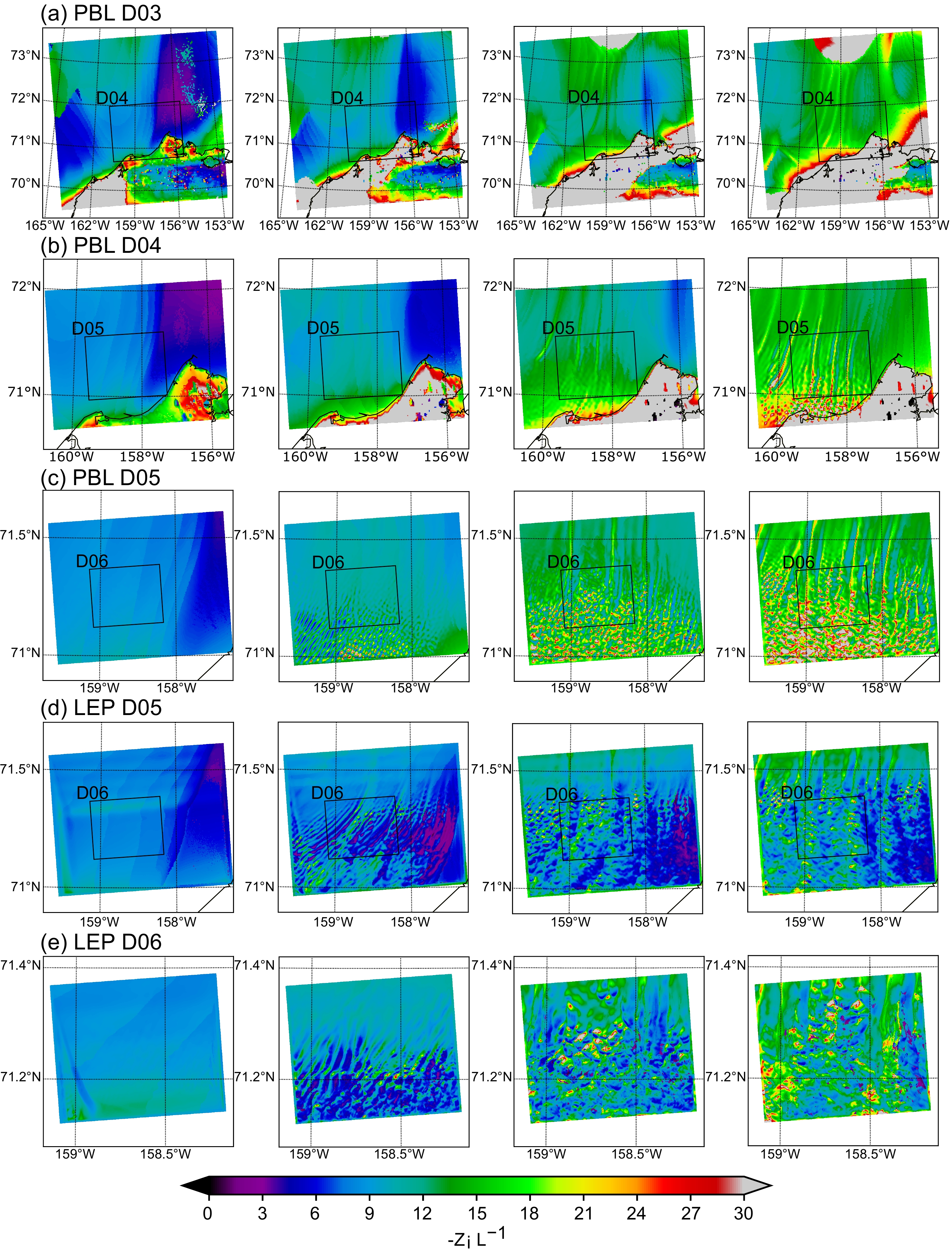
where θ_v is the surface air virtual potential temperature, u_* is friction velocity, k is the von Kármán constant, g is gravitational acceleration, and ${\left({\overline {w'\theta '} } \right)_{{\rm{sfc}}}}$ is the surface heat flux. Previous studies have demonstrated that −Z_i/L can be used to quantify the instability associated with the transitions between roll- and cell-type clouds (Deardorff, 1972; Weckwerth et al., 1997, 1999; Khanna and Brasseur, 1998). Based on observations Weckwerth et al. (1999) suggested that the transition from rolls to cells generally occurs around −Z_i/L ~ 25, whereas Salesky et al. (2017) suggested that the transition occurs in the range of −Z_i/L ~15−20 in LESs. Here, we applied −Z_i/L to quantify the state of the boundary layer associated with the formation of the roll clouds observed in this study.

Figure 6 shows the evolution of model-produced roll-like structures in −Z_i/L to the west of Utqiaġvik centered near 71.5°N and 159.0°W in all of the domains. For the results in this figure the boundary layer depth was defined by the height of the temperature inversion in the vertical temperature profiles. We took the second derivative of the vertical temperature profiles at each grid location and found the minimum values that resulted; the heights of these values were taken to be Z_i. In the beginning (left column in Fig. 6), the values of −Z_i/L were consistent through all the model domains. At the next hour, roll-like structures developed within the downstream (southern) parts of domains PBL D05, LEP D05, and LEP D06 where the values of −Z_i/L were smaller than for the upstream (northern) parts of the domains. When the roll-structures developed, the stability changed differently among the domains. In domain PBL D03 the values of −Z_i/L changed from a range of 8 to 11 to a range of 12 to 19 near the rolls to the west of Utqiaġvik (first row in Fig. 6). As spatial resolution increased from domain PBL D03 to domains PBL D04 and PBL D05, the range of −Z_i/L widened to approximately 12–25 in the vicinity of the rolls. To the south of 71.5°N and 159.0°W, −Z_i/L often exceeded 25, and in this region the roll structures gave way to more cell-type clouds. The roll structures were similar in the northern parts of domains PBL D05 and LEP D05, although the values in PBL D05 were greater than in LEP D05. These similar patterns were caused by large-scale features propagating from the parent domains. Therefore, we focused on the results from the middle of the domains. As a result of the unstable environment near the surface (decreasing potential temperature with height) within these domains (Fig. 5a), the boundary layer was positively buoyant near the surface in this region. In domains LEP D05 and LEP D06, for which the PBL scheme was turned off, values of −Z_i/L decreased to as low as 6 in some locations, indicating more shear-driven convection in these regions within these domains. Comparing the individual ${\left({\overline {w'\theta '} } \right)_{s{\rm{fc}}}}$, u_*, and Z_i components, the increase of u_* with decreasing grid spacing was the main factor behind changes in the magnitude of −Z_i/L. The wavenumber of the roll structures from domain PBL D03 down to LEP D06 also increased with increasing spatial resolution. For example, domain PBL D04 within PBL D03 (black box in Fig. 6a) had the five dominant roll structures evident in PBL D03, plus many additional finer resolution rolls in between (Fig. 6b). Overall, more rolls were produced with increasing model spatial resolution.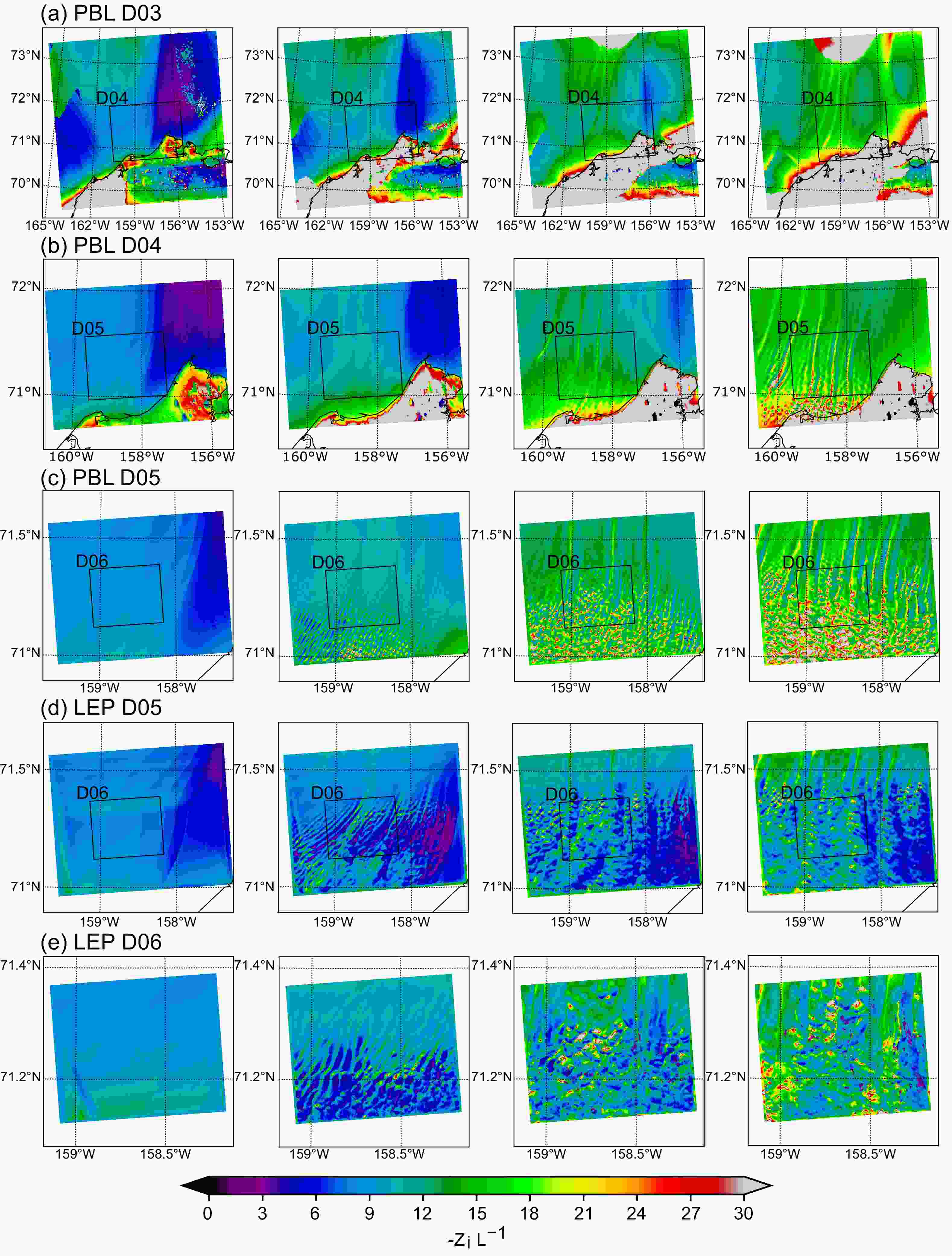

Figure 6.  Boundary layer values from 1900 UTC to 2200 UTC (left to right) on 1 May 2013 of the ratio −Z_i/L in WRF domains (a) PBL D03, (b) PBL D04, (c) PBL D05, (d) LEP D05, and (e) LEP D06.

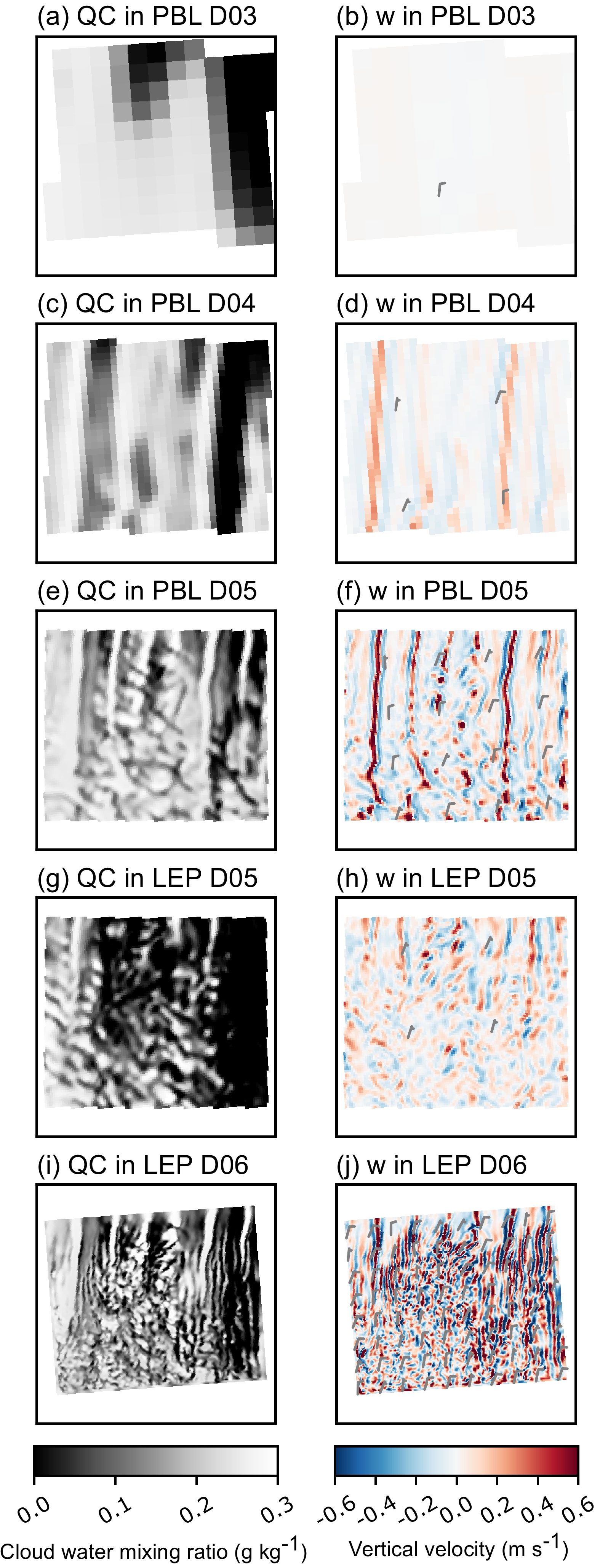
Cloud streets can be aligned parallel to the wind shear vector, perpendicular to it, or at angles in between depending on boundary layer conditions (Asai, 1970a,b ). From the last subsection, the model produced a convectively heated boundary layer with different degrees of stability. For example, the −Z_i/L values presented in Fig. 6e for LEP D06 correspond to the vertical velocities in LEP D06 presented in Fig. 7j. The roll structures were more organized in regions with −Z_i/L < 20 than in regions with −Z_i/L > 20. These results indicate that the roll-like structures depended on the instability within the boundary layer and the model produced suitable environments for rolls to develop. In this case, horizontal cross sections of boundary-layer-top cloud water mixing ratio at 500 m (Fig. 7, left column) show the rolls aligned parallel to the wind direction in all of the domains (Fig. 7, right column). The clouds were stratiform-like in the coarser domain PBL D03 (Fig. 7a), and as the spatial resolution of the domains increased, roll-like structures with ever smaller wavelengths appeared. The coarser resolution domains had cloud fractions close to 1 across most of domain LEP D06 (Fig. 3). In the vicinity of the rolls in domain LEP D06, gaps in the clouds opened up along the streets of descending air and overall cloud fraction decreased. The structure of organized rolls in LEP D05 was similar to PBL D05, but the cloud water mixing ratio was lower with more cloud-free areas in the LEP run, especially in the eastern part of the domain (Fig. 7e, g). The differences in cloud-water mixing ratios in this region were associated with differences in boundary layer stability. Figures 6c and d show larger −Z_i/L values to the east in the PBL domain than in the LEP domain. In this case, clouds in PBL D05 were likely the result of convective instability, whereas less cloud-water mixing ratios were produced in LEP D05 because of a less unstable boundary layer and weaker vertical motions (Fig. 7h). Although domain LEP D06 was less unstable compared to the PBL domains, the modeled vertical motions were stronger in LEP D06 (Fig. 7j) due to stronger wind shear, which enhanced cloud formation in the eastern parts of domain D06.

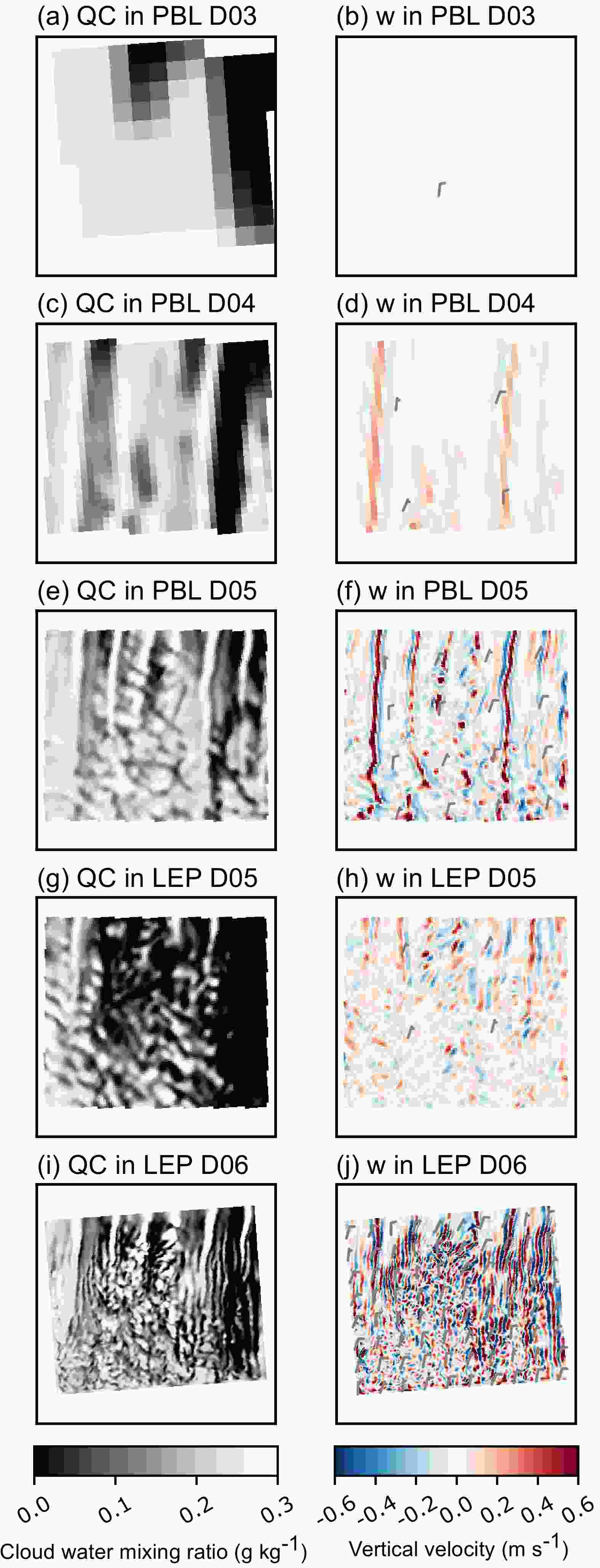
Figure 7.  Horizontal cross sections of cloud water mixing ratio and vertical velocity across the region covered by domain D06 taken from WRF domains (a, b) PBL D03, (c, d) PBL D04, (e, f) PBL D05, (g, h) LEP D05, and (i, j) LEP D06 at a height of 500 m at 2200 UTC 1 May 2013. The grey barbs indicate the horizontal winds.

As expected, vertical velocities strengthened as the domain grid spacing decreased (and the resolution increased). The right column of Fig. 7 presents the horizontal distribution of vertical velocities for all of the domains, again across the region covered by domain LEP D06. As the grid spacing decreased, the wavelengths of the roll structures also decreased. Compared with PBL D05, the vertical velocities in LEP D05 were weaker, but still contained line structures (structures that were readily apparent in LEP D06). The lack of strong vertical velocities within the cloud-free region in LEP D05 indicates that LEP with 0.333-km grid spacing might be too coarse to produce sufficiently strong vertical motions for cloud formation in this case.

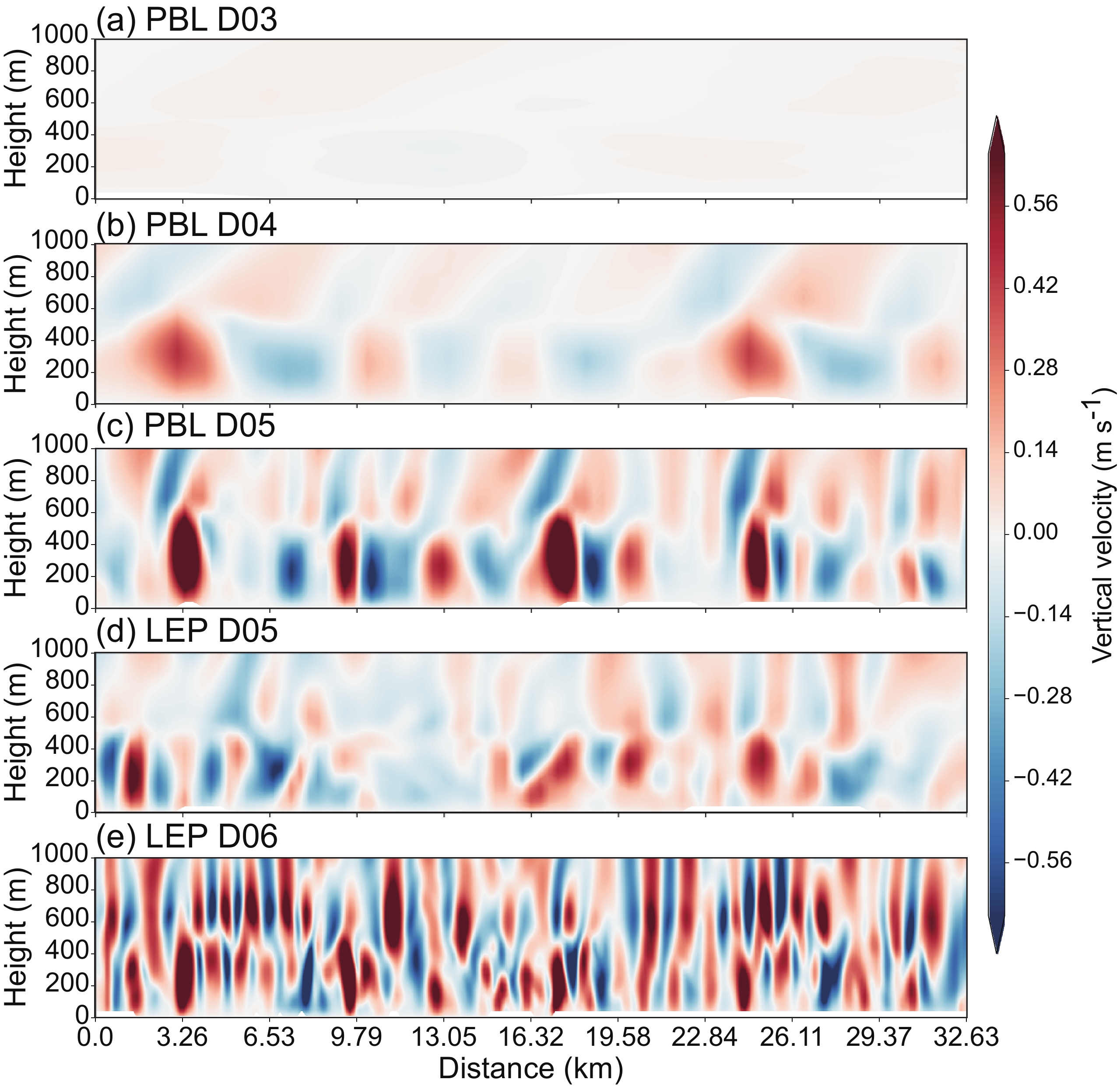
Vertical cross sections of vertical velocity from the different model domains indicate that there were different types of waves generated within the model (Fig. 8). The wave-like structures within the boundary layer (below 500 m) were rolls and the waves above the boundary layer were most likely gravity waves induced by the rolls. From domain PBL D03 to domain LEP D06 the boundary layer waves appeared with different wavelengths. Overall, vertical velocities increased in magnitude as the waves decreased in wavelength, as expected. The vertical velocities in LEP D05 were slightly weaker from near the surface to 1000-m heights than in PBL D05 (Figs. 8c and d). Below 500 m, LEP D05 produced rolls with weaker vertical velocities and smaller wavelengths. These results indicate that LEP D05 simulated roll features with larger wavenumbers than PBL D05 with the same horizontal spatial resolution but with poorly represented turbulent motions.

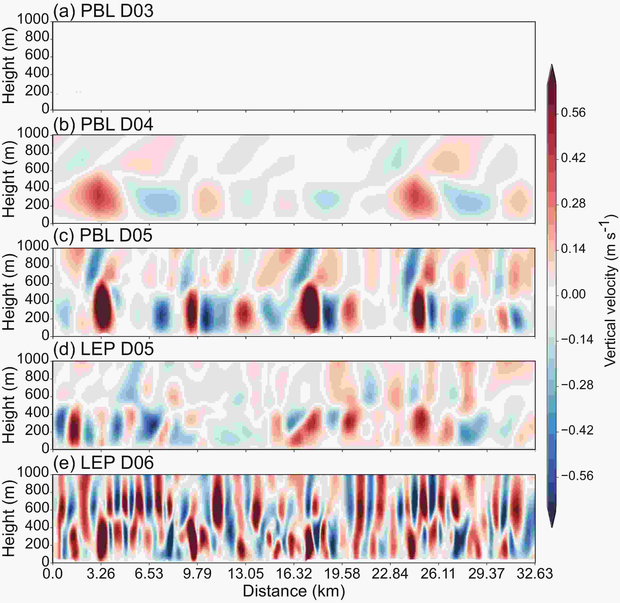
Figure 8.  West to east vertical cross sections of vertical velocity at 2200 UTC 1 May 2013 located across the middle of domain D06 but for WRF domains (a) PBL D03, (b) PBL D04, (c) PBL D05, (d) LEP D05, and (e) LEP D06.

Simulated cloud properties were affected by varying the grid spacing. Figure 9 presents west to east vertical cross sections of cloud-water mixing ratio across the middle of domain D06. The clouds were stratiform-like in the coarser domain PBL D03 (Fig. 9a). As the spatial resolution of the domains increased, roll-like structures with ever smaller wavelengths appeared, i.e., the wavelengths of the roll clouds decreased with decreasing grid spacing. With increasing horizontal spatial resolution cloud-water mixing ratios, cloud-base heights, and cloud-top heights became more variable. In domains PBL D05 and LEP D05 the average cloud-top and cloud-base heights were similar but their cloud structures were slightly different. Thus, overall cloud properties were not affected significantly by changing from the PBL scheme to LEP in this case, likely due to LEP D05 marginally resolving the rolls.

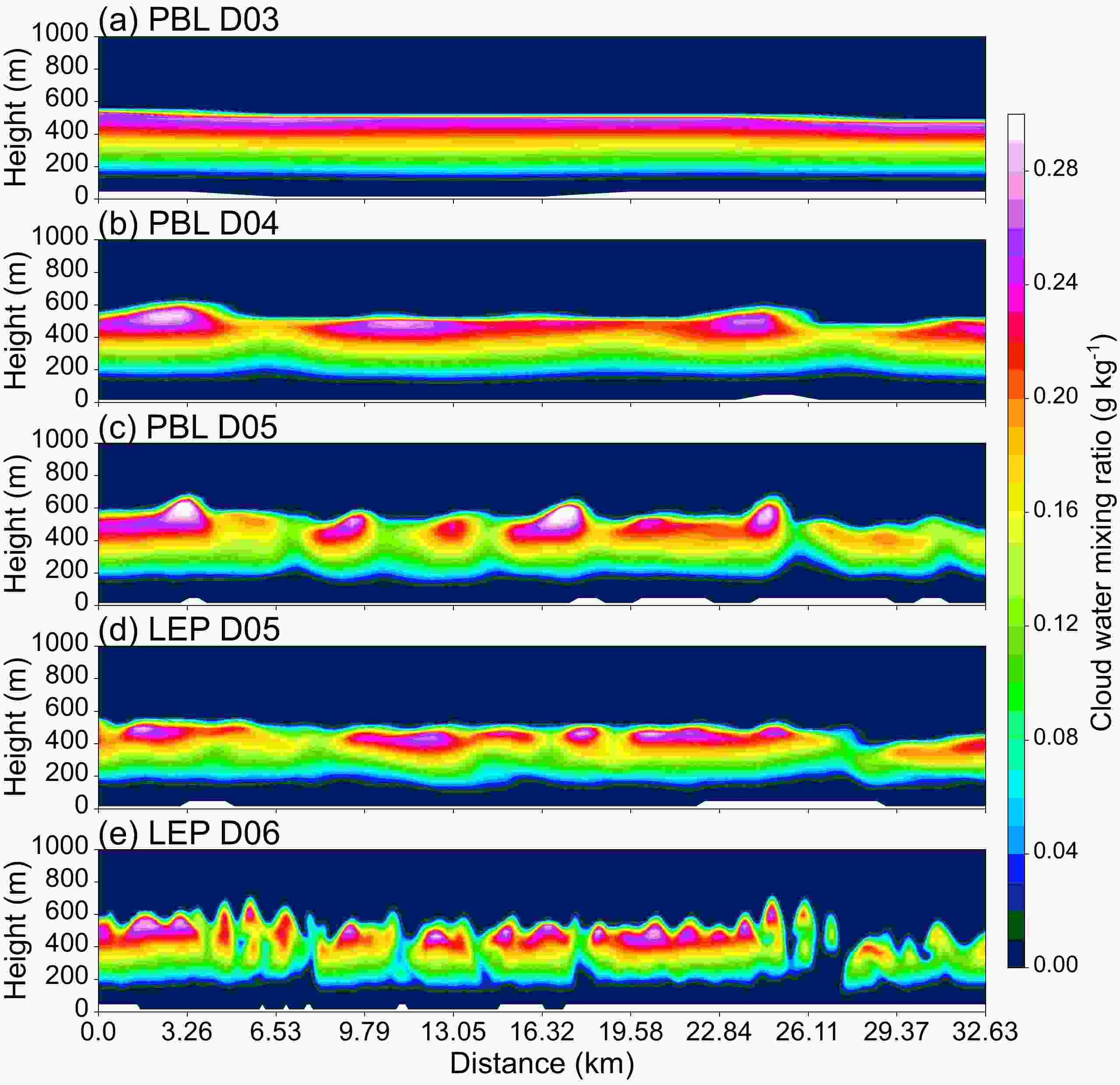
Figure 9.  West to east vertical cross sections of cloud water mixing ratio at 2200 UTC 1 May 2013 located at the middle of domain D06 but for WRF domains (a) PBL D03, (b) PBL D04, (c) PBL D05, (d) LEP D05, and (e) LEP D06.

Figure 10a shows the west to east vertical cross section of water vapor mixing ratio in domain PBL D03 across the middle of domain D06. Water vapor was stratified in PBL D03 and increased both with decreasing height below 500 m and increasing height above the cloud layer (500 m, Fig. 9a). Figures 10b, c and e show a significant decrease of water vapor mixing ratio below 100 m to near the surface and an increase of water vapor mixing ratio within the cloud layers as the spatial resolution increased. These results indicate that the model produced a stronger vertical water vapor gradient below the cloud layer with decreasing grid spacing. As the spatial resolution increased, more water vapor was transported from the surface to the cloud layer because of stronger vertical motion within the boundary layer (Fig. 8). Furthermore, more water vapor was transported to above the cloud layer, perhaps as a result of more in-cloud turbulent mixing across the cloud top. In domain LEP D05 the increasing water vapor mixing ratio within the cloud layer was not significant, although the decrease in water vapor near the surface was (Fig. 10d).

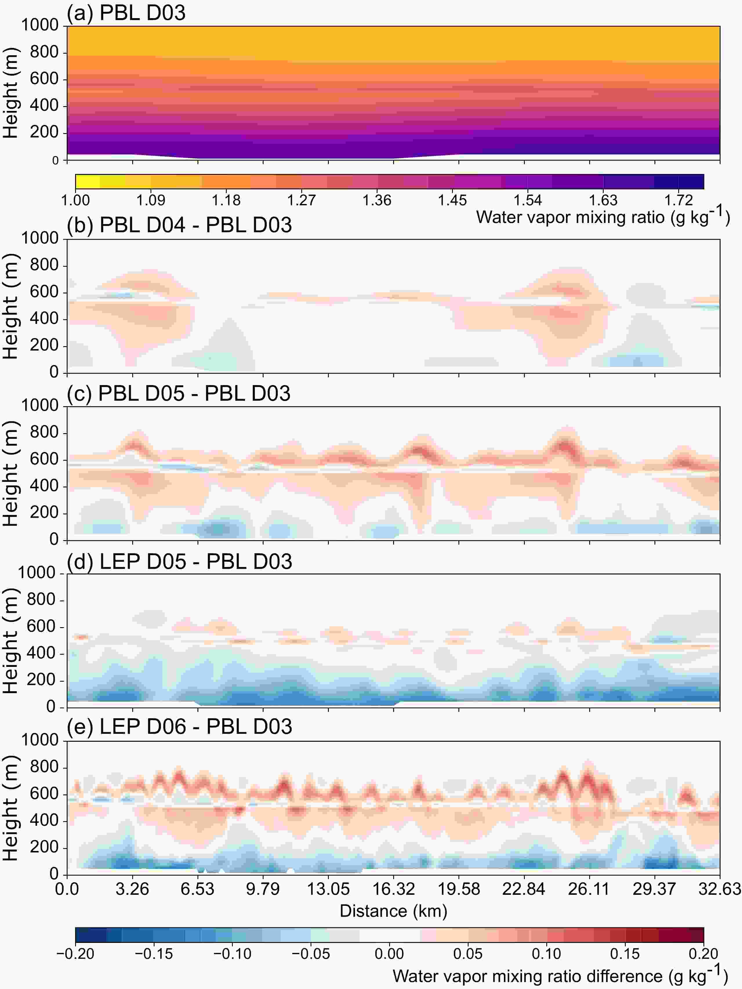
Figure 10.  West to east vertical cross sections across the middle of domain D06 of (a) WRF simulated water vapor mixing ratio in domain PBL D03 and simulated water vapor differences relative to domain PBL D03 of domains (b) PBL D04, (c) PBL D05, (d) LEP D05, and (e) LEP D06 at 2200 UTC 1 May 2013.

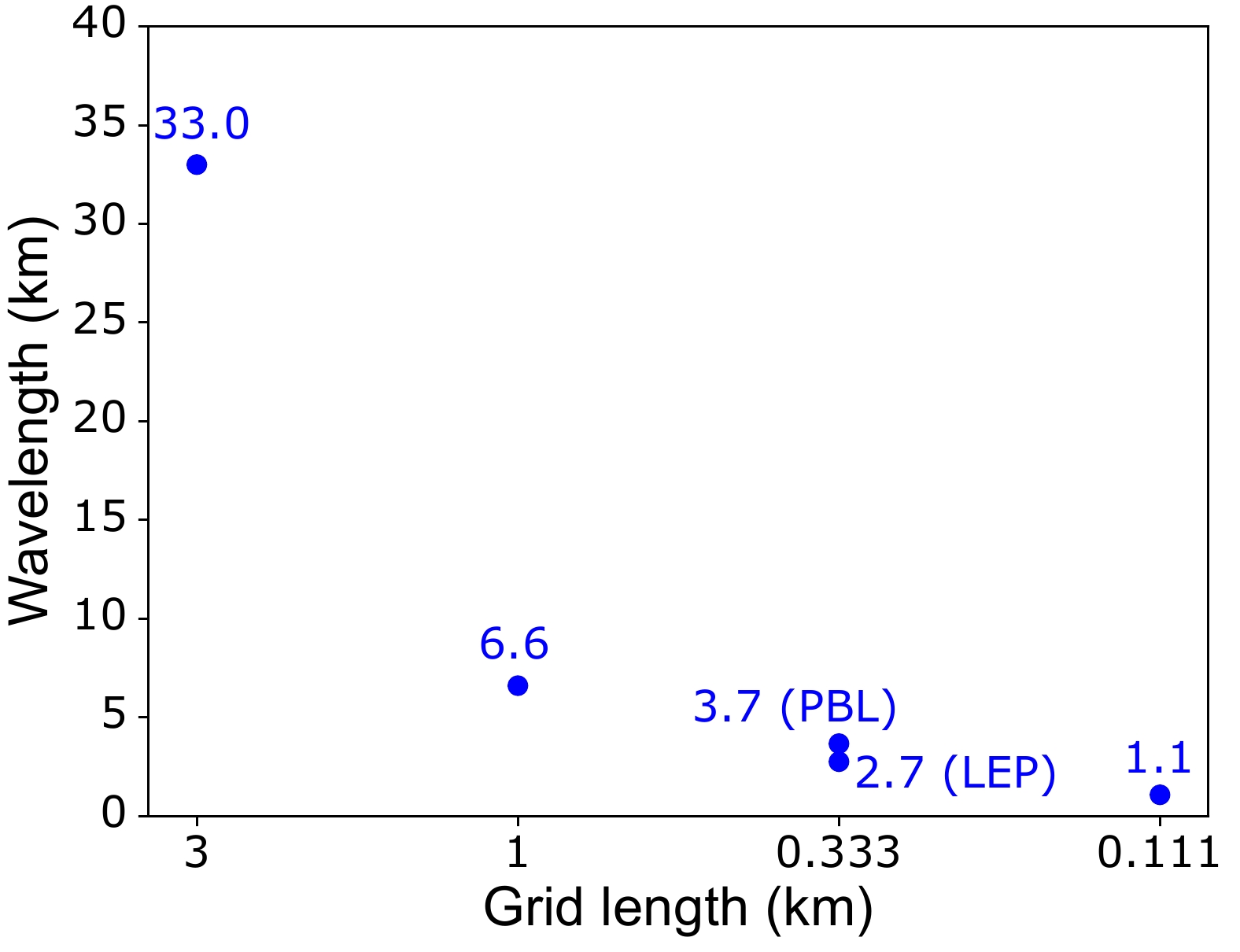
We applied a fast Fourier transform to the vertical velocities within the PBL at 400-m heights in the vertical cross sections illustrated in Fig. 8 to obtain the dominant spatial wavelengths that contributed to the wave structures. The dominant wavelength, resulting from the roll features, decreased from 33.0 km to 1.1 km as the grid spacing decreased from 3 km to 0.111 km, respectively (Fig. 11). Switching from the PBL D05 to the LEP D05 with the same 0.333-km grid spacing led to a decrease of 1 km in roll cloud wavelength. The MODIS-observed roll clouds had wavelengths from 2.5–2.8 km, which fall closest to the LEP D05 wavelength of 2.7 km and in between the PBL D05 wavelength of 3.7 km and the LEP D06 wavelength of 1.1 km. These results indicate that model domains PBL D05 and LEP D05 produced similar rolls. However, the boundary layer height was about 500 m in this study, implying that domain D05 with horizontal grid spacing of 0.333 km could be too coarse to resolve turbulence within the boundary layer. On the other hand, LEP D06 had sufficiently small grid lengths to resolve the roll clouds observed within the boundary layer during this case study period. Aspect ratios (i.e., roll wavelength divided by boundary layer depth) of observed cloud streets show a wide range from 1.8 to 12.1 (Young et al., 2002). In our case the aspect ratios of the simulated rolls in LEP domain D06 were about 2.2 and consistent with observed values. Despite the dominant wavelength in LEP D06 being smaller than the observed wavelength, the simulated cloud-base height was also lower than the observed height, which could explain the wavelength difference (Figs. 4a and 9). Although PBL D05, LEP D05, and LEP D06 all produced roll structures that are similar to the observed rolls, the mechanisms of cloud formation (according to −Z_i/L), cloud microphysical properties, and boundary layer structure (e.g., stability and vertical fluxes) were slightly different among them. It is beyond the scope of the current study to fully understand the numerics, physics, and parameterizations under different grid spacings that led to the differences among different domains, except to point out their apparent inadequacy in resolving the observed roll clouds with the exception of LEP D06 with 111-m grid spacing. It is also beyond the scope of the current study to fully explore what other deficiencies, either from initial and boundary conditions or other sources of model physics uncertainties, might be responsible for the differences in simulated rolls within LEP D06 and those that were observed, despite the use of adequate horizontal resolution. Predictability of these smaller scale roll clouds might be inherently limited due to the chaotic nature of moist processes—the smaller the scale, the less their predictability (Zhang et al., 2019).

Figure 11.  Roll-cloud simulated wavelengths at 2200 UTC 1 May 2013 versus WRF horizontal grid spacing of 3 km (PBL D03), 1 km (PBL D04), 0.333 km (PBL D05 and LEP D05), and 0.111 km (LEP D06).

We investigated the sensitivity of simulated Arctic roll clouds and boundary layer structures to model horizontal resolution and to the switch from a PBL scheme to an LEP configuration. We chose a case of low-level roll clouds that were observed about 90 km to the west of the DOE ARM Climate Research Facility at Utqiaġvik, Alaska, on 1–2 May 2013. The focus of this study was to use a cloud-resolving weather model initialized from realistic atmospheric conditions to model the clouds at the grey zone between the mesoscale and large-eddy scale. To this end, we used six one-way nested domains within the WRF model to simulate the roll clouds and the boundary layer conditions in which they occurred.

We compared the large-scale environment between the outer model domains and observations and found that the model was able to reproduce a similar boundary layer structure as observed. We further examined WRF simulation output in the inner domains and found that the stability of the boundary layer changed from the mesoscale to large-eddy permitting scale. Virtual potential temperature profiles changed from slightly unstable to stable with increasing model horizontal resolution. Analysis of horizontal cross sections of the stability parameter −Z_i/L over domains PBL D03 through LEP D06 shows a transition from a more buoyant-driven boundary layer to a less unstable boundary layer, mainly due to increasing friction velocity near the surface with decreasing grid spacing. Domains PBL D05 and LEP D06 presented roll clouds that were more similar to the observed rolls though being intermediate between a pure convective case and a pure shear-driven case. Domain LEP D06 was able to model roll clouds with a wavelength of 1.1 km within a less unstable environment whereas PBL D05 produced rolls with a dominant wavelength of 3.7 km but within a more convective environment.

Clouds transitioned from stratiform- to roll-like structures with decreasing grid length and the wavelengths of the rolls decreased. The vertical distribution of water vapor mixing ratios also changed with decreasing grid length. In the layer between the in-cloud and above-cloud layers, the water vapor mixing ratios increased with increasing model resolution. From the near surface to the cloud layer, the vertical gradient of water vapor mixing ratios also increased with increasing horizontal resolution.

Keeping the same model resolution but changing from the PBL to LEP domain within the grey zone led to a more shear-driven, less unstable environment. In addition, the profiles of virtual potential temperature, water vapor mixing ratio, and winds below the cloud layers were more affected by this change than changes in model resolution. The dominant roll-cloud wavelength was smaller in LEP D05, but line structures in the vertical velocity were not as strong as for PBL D05. Nevertheless, the cloud structures in these two domains were similar to each other though boundary layer properties within them were fairly different. The LEP D05 may not well resolve the turbulence-produced weaker vertical velocities and smaller cloud-water mixing ratios that were found in PBL D05.

The wavelengths of the simulated roll clouds were 3.7 km, 2.7 km, and 1.1 km for domains PBL D05, LEP D05, and LEP D06, respectively, covering the MODIS-observed wavelengths ranging from 2.5 km to 2.8 km. The number of grid points necessary for resolving the wave features was about 7 to 10 grid points. In this study, a LEP domain with a grid spacing of 0.111 km nested within a PBL domain with 0.333-km grid spacing was sufficient to model observed roll clouds with wavelengths of 2.5–2.8 km.

A limitation of this study is that it was difficult to compare directly the model output with available observations. Ground-based measurements can provide detailed information about boundary layer conditions, but are often point measurements and representative of very small scales. Satellite observations can be useful for validating model results (e.g., Field et al., 2017), but space-borne measurements struggle to provide information about boundary layer profiles. More regional observations would be helpful to verify the model results. Furthermore, additional future sensitivity studies on different boundary layer environments could help to generalize the impact of model grid spacing on cloud dynamics and thermodynamics, especially for the grid spacing within the grey zone.

Although WRF was able to simulate cloud features with many attributes comparable to the observations, in our set of simulations WRF never produced clouds composed of frontal clouds together with cloud streets as observed. We tried different microphysical schemes, PBL schemes, and radiation schemes in the WRF model; however, we never found a configuration that produced the long-lived cloud systems with underlying rolls as observed for this case. We also ran an idealized LES in WRF based on an observed sounding from Utqiaġvik, Alaska, during a period in which cloud streets were found under stratocumulus clouds. The LEP domain produced multilayered clouds in the beginning of the simulation, but the development of turbulence quickly eroded the pocket of stability in which the low-level clouds formed after which they disappeared. Future WRF simulations will be used to investigate the production of cloud streets with the frontal clouds for this case study period.

Acknowledgements. This work was supported by the U.S. DOE ASR (Atmospheric Systems Research) program (Grant No. DE-SC0013953). The measurements used in this study were obtained from the U.S. DOE ARM user facility and NASA LAADS (Level-1 and Atmosphere Archive & Distribution System) DAAC (Distributed Active Archive Center). The computing was performed at the Texas Advanced Computing Center. We would like to thank Dr. Jerry HARRINGTON for fruitful discussions.