


 DownLoad:


-
Surface observation data are a critical component of the High-Resolution China Meteorological Administration's Land Assimilation System (HRCLDAS). At present, the number of national meteorological stations is more than 2400, and the number of regional automatic stations is approximately 60 000. To obtain high-resolution and high-quality assimilation products, it is necessary to assimilate large amounts of surface observation data. However, before 2008, due to the sparsity of meteorological stations in China, it was impossible to obtain surface observation data with high coverage. Taking the national reference stations and national basic stations as an example, the number of the stations was less than 100 in 1930, between 100 and 200 in the 1930s and the mid-1940s, dropping to less than 100 between the mid-1940s and early 1950s, before finally increasing to approximately 2400 in 2020. Since 2008, the China Meteorological Administration has set up more than 60 000 encrypted automatic stations. As noted above, the available observational data are insufficient to allow HRCLDAS to back-calculate the high-resolution assimilation data before 2008. We think deep statistical downscaling provides one potential method to accurately reconstruct high-resolution data, which could be used to fill in the product gaps in HRCLDAS, especially before 2008. Therefore, this research established a super-resolution deep learning model that attempts to generate high-resolution data. This work is applicable to high-resolution technology research in general as well as to potential future work that could back-calculate assimilation data and help fill in the data gaps caused by sparse meteorological stations prior to 2008.
Our model uses super-resolution technology for reference because Statistical Downscaling (SD) in meteorology is similar to the Super-Resolution (SR) in computer vision. The former establishes a nonlinear mapping relationship between element fields in different scales (this nonlinear relationship is affected by various atmospheric physical factors); the latter involves recovering image degradation (such as blur and noise) because of the channel propagation process. The similarity between these methods is that they are intended to convert a mapping from coarse (low-resolution) images (fields) to fine (high-resolution) images (fields). In recent years, deep-learning-based, super-resolution technology has been booming, opening up new ideas for many statistical downscaling studies. For example, Vandal et al. (2017) stacked multiple super-resolution convolution neural networks (SRCNN, Dong et al., 2014) and proposed the first deep-learning-based downscaling model, deep statistical downscaling (DeepSD, Vandal et al., 2017), to perform precipitation downscaling tasks with different scaling factors. Mao (2019) modified DeepSD, added a residual structure, deepened the network depth, and proposed the very deep statistical downscaling model (VDSD). Cheng et al. (2020) proposed the numerical weather prediction multi-time super-resolution model (NWP-MTSR) to downscale the precipitation field. Singh et al. (2019) verified the portability of the generative adversarial network model to the enhanced super-resolution generative adversarial networks (ESRGAN, Wang et al., 2019) in a wind field downscaling task.
The resolution of most previous field reconstructions was relatively coarse (approximately 0.05° × 0.05°), and the spatial geomorphic feature information was not detailed enough. Compared with the previous similar statistical downscaling works based on deep learning, our study aims to back-calculate the 0.01° × 0.01° resolution product from HRCLDAS. Therefore, we propose the China Meteorological Administration's Land Assimilation System Statistical Downscaling Model (CLDASSD) to downscale the 2-m temperature product (0.0625° × 0.0625°) from CLDAS and reconstruct higher-resolution (0.01° × 0.01°) temperature products.
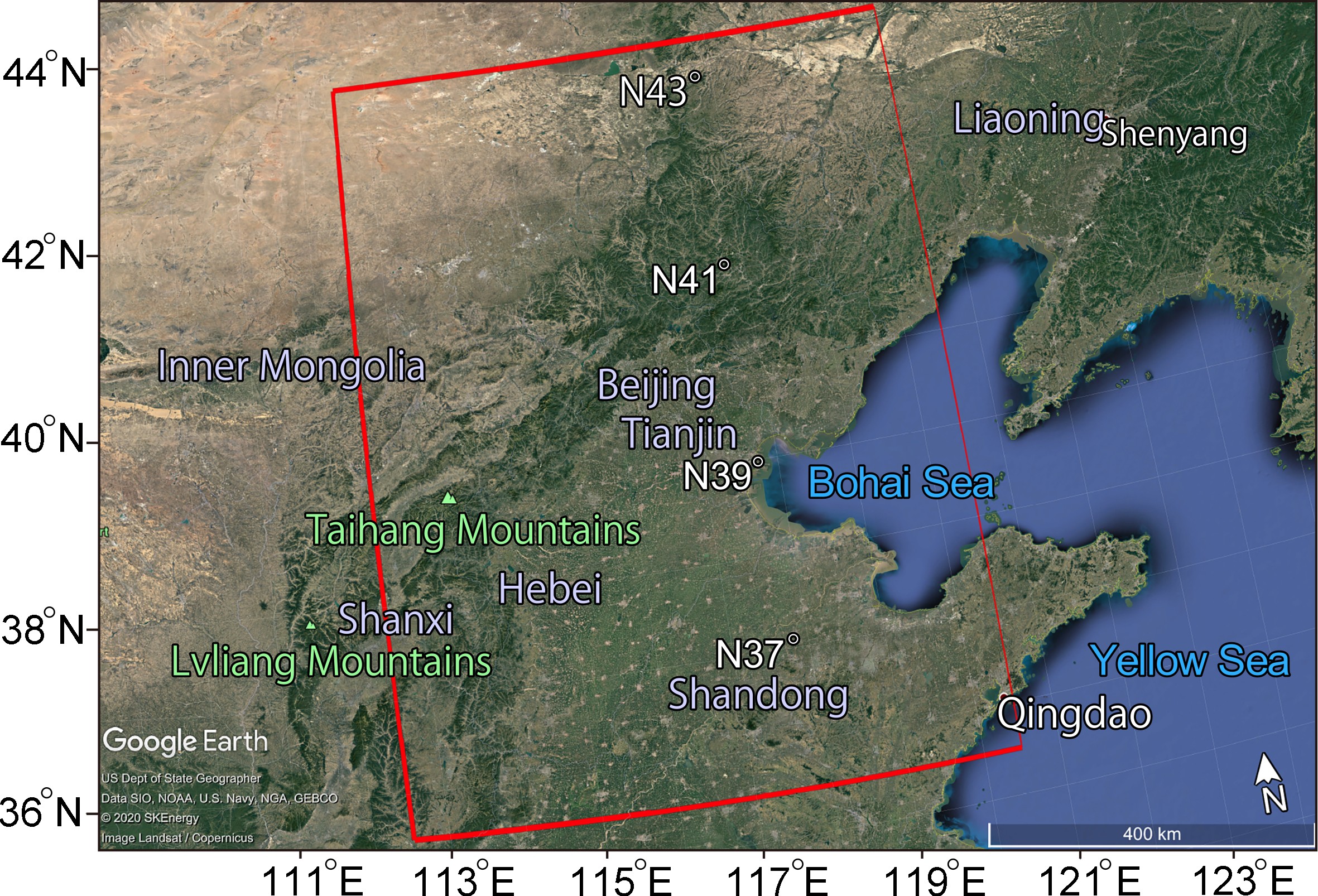
Before the experiment, we performed a statistical analysis of the paired data from CLDAS and HRCLDAS. Then, we explored the quality control methods of the data. In the model training and testing stage, through comparative experiments and ablation experiments, we took the data from HRCLDAS and surface observation data as “true values” to evaluate the performance of CLDASSD. Our experimental area is the Beijing-Tianjin-Hebei region which has complex and diverse geomorphology and is located at the heart of the Bohai Rim in Northeast Asia and China (35.5°–43.5°N, 112.5°–120.5°E). Figure 1 shows the geographical location and topography of the area, which contains various landforms, such as water bodies, mountains, and plains.
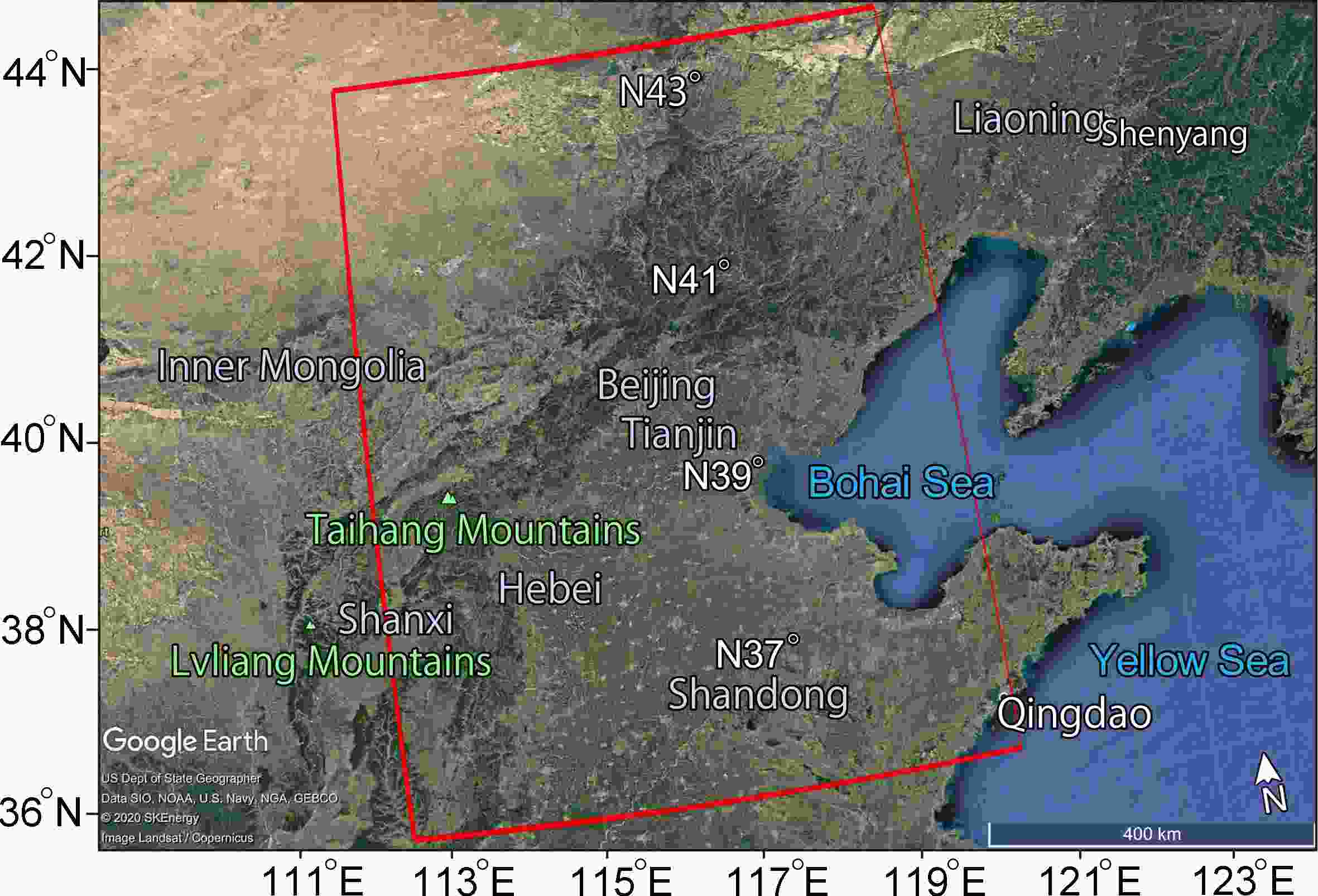
Figure 1. A map of the Beijing-Tianjin-Hebei region assembled from high-definition satellite maps provided by Google Earth. The red box delineates our test area, in which the plateau in the northwest, the mountains in the middle, the plains in the south, and the Bohai Bay in the east are visible.
The remainder of this paper is organized as follows: Section 2 describes the datasets used in this study, section 3 describes the methodology of the downscaling technique, section 4 provides the results and associated discussion and, section 5 summarizes the research.
-
The inputs of CLDASSD are a low-resolution temperature field and a high-resolution digital elevation model (DEM). The output is the corresponding high-resolution temperature field.
The low-resolution, 2-m temperature data come from CLDAS-Version 2.0. The data are a grid fusion product covering the Asian region (0°–65°N, 60°–160°E) with a spatial resolution of 0.0625°, of equal latitude and longitude grids, and at a temporal resolution of one hour. This dataset uses multiple ground and satellite observation data sources and technologies, such as multigrid variational assimilation (STMAS), cumulative probability density function matching (CDF), physical inversion, terrain correction, and other technologies. The associated quality is better than that of similar international products in China (Han et al., 2020).
The CLDASSD target temperature data come from HRCLDAS-Version 1.0, newly developed by the National Meteorological Information Center. The hourly grid fusion product set with a resolution of 0.01° includes surface pressure information, approximate 2-m temperature, 2-m specific humidity, precipitation, 10-m wind speed, and solar shortwave radiation (Han et al., 2019). The grid products of temperature, pressure, humidity, and wind speed are realized mainly by fusing European Centre for Medium-Range Weather Forecasts (ECMWF) analysis and forecast field data with observation data from more than 40 000 stations across the country through the STMAS method (Shi et al., 2019).
The 0.01° DEM data over China are derived from 90-m-resolution terrain data from the National Aeronautics and Space Administration's shuttle radar topographic mission. At this resolution, most mountains, rivers, and plains can be well represented.
In the selected experimental area, the numerical matrix shape of the 0.0625° × 0.0625° temperature field is 128 × 128, and the shapes of the 0.01° × 0.01° temperature field and 0.01° × 0.01° DEM data are both 800 × 800. Considering the total amount of data and to account for intra-day differences, we selected the paired data at UTC 0000, 0600, 1200, and 1800 from CLDAS and HRCLDAS to construct the experimental database.
To make reasonable use of GPU resources, we used a sliding window to crop the samples to many small patches. Thus, in the paired patches, the area of the low-resolution patches is 16 × 16. The area of the high-resolution patches and DEM patches is 100 × 100. We use this size because if the patch size is too large, it will occupy excessive GPU memory, whereas one that is too small cannot capture the associated spatial information (Wang et al., 2020). We arrived at an acceptable patch size through many tests.
The time range of the entire database is from January 2018 to December 2019. The data from 18 March to 19 February were used as the training set (we extracted 10% according to the time and season as the validation set). The remaining data were used as a test set to evaluate the performance of the model.
-
The 0.0625° scale and the 0.01° scale are of the same synoptic scale, so there should be no systematic error between these two scales of products. However, a specific Gaussian random error exists between them (there are many physical influence factors, with each influence factor having minor effects). The error can be obtained from the central limit theorem. Nevertheless, our experimental data come from different assimilation systems (low-resolution data from CLDAS, high-resolution data from HRCLDAS), and a small amount of paired data may have a systematic error.
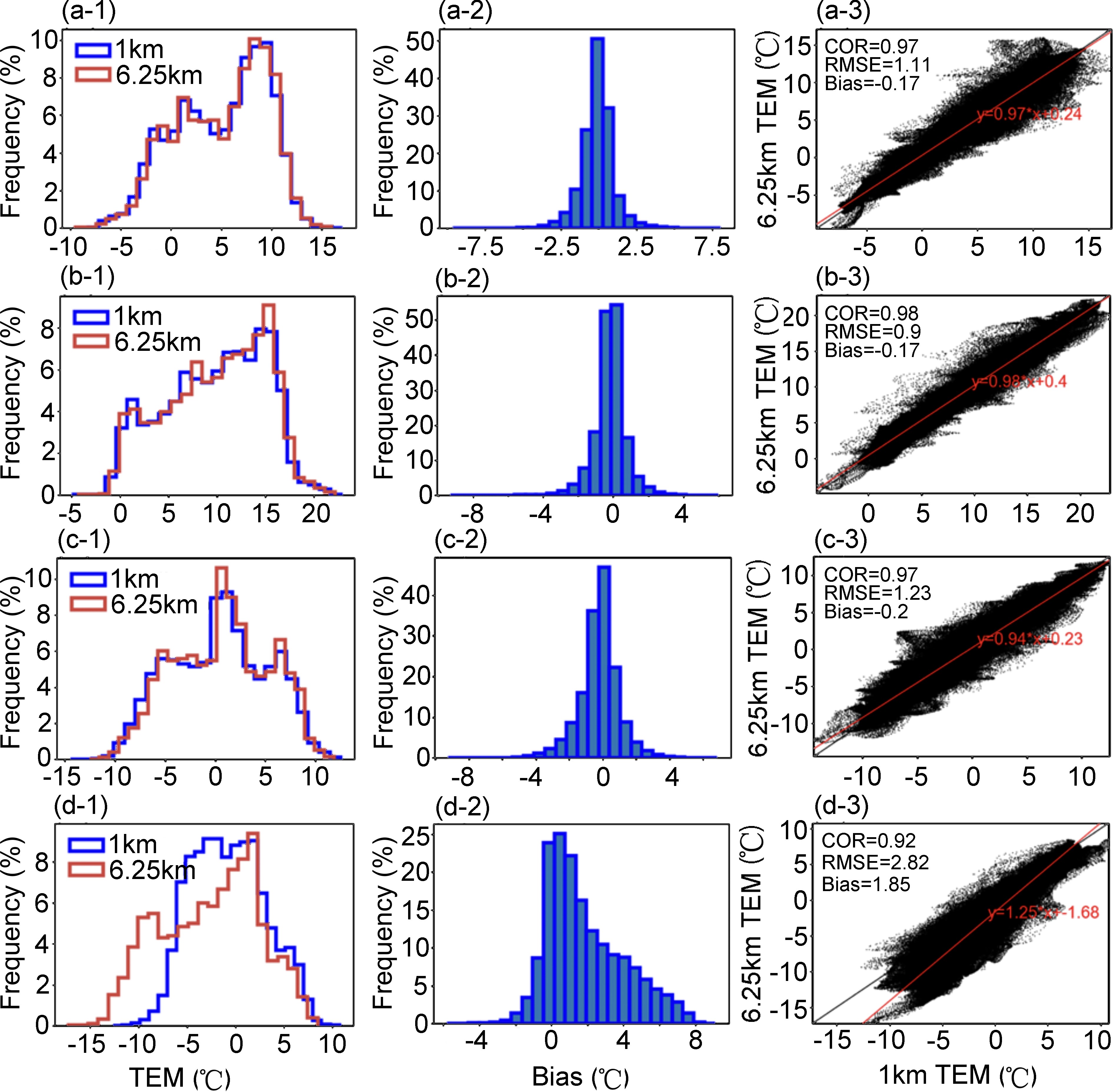
Taking the temperature product on 10 March 2018, as an example, Fig. 2 shows that at 0000, 0600, and 1200 UTC, the distributions between the high- and low-resolution fields are highly consistent, and the correlation coefficients (COR) between them are close to 1. Furthermore, the root mean square error (RMSE) is approximately 1°C, and the residual error obeys a normal distribution with a mean close to 0. In contrast, at 1800 UTC, the distribution differs considerably between the high- and low-resolution fields. The residuals show a skewed distribution, and the COR is lower than in the other samples. The RMSE is close to 3°C. This type of sample is considered to be poor-quality data and is to be eliminated before conducting experiments. The generation of such dirty data depends on the stability of HRCLDAS and the quality of the background field. Their data distribution is different from most samples. If we do not delete them, this will prevent the model from focusing on learning from those high-quality data distributions, thereby affecting the final performance of the model.
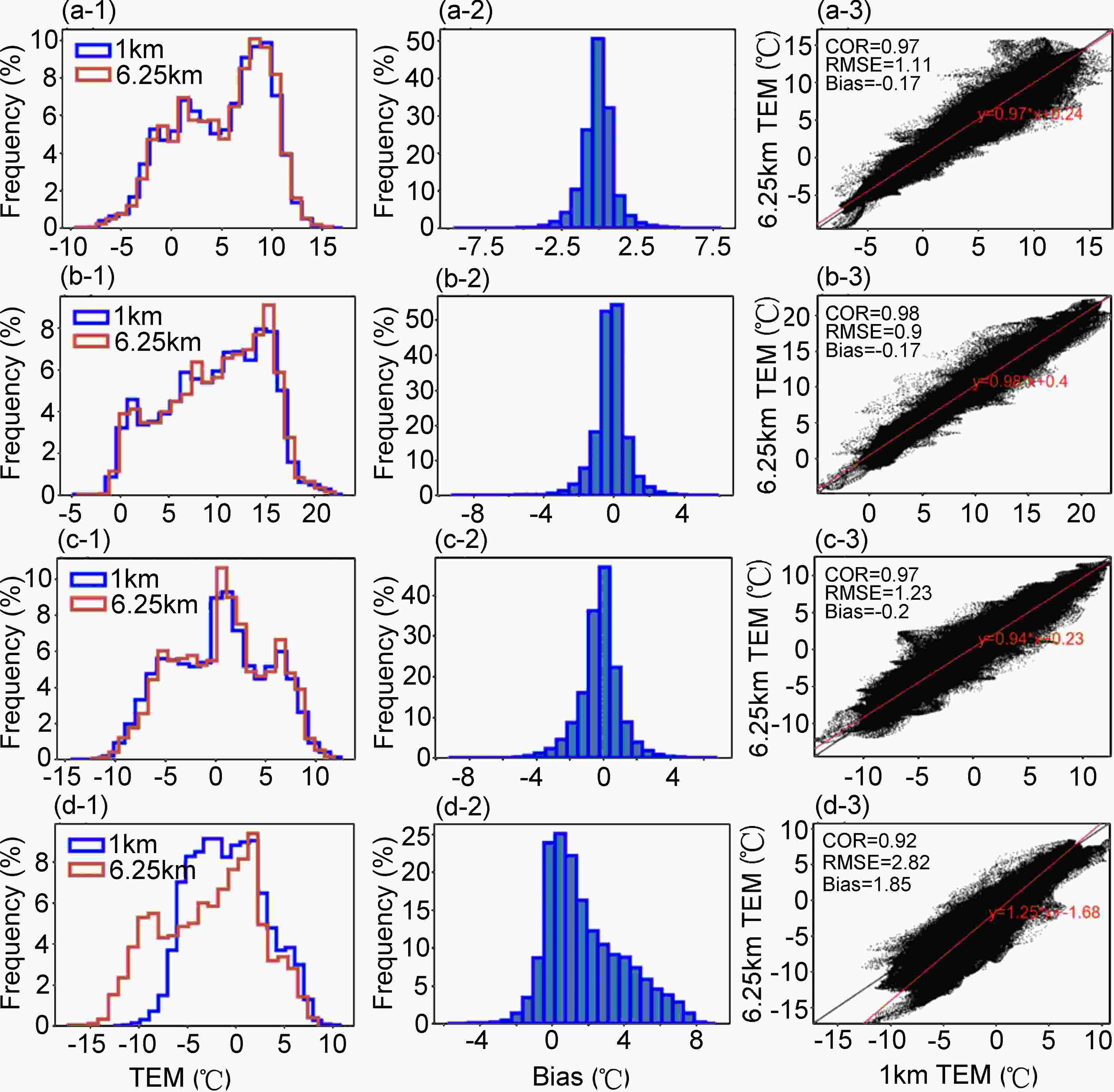
Figure 2. Graphical displays of the paired data from CLDAS (the spatial resolution is 0.0625° × 0.0625°) and HRCLDAS (0.01° × 0.01°) on 12 May 2018, as an example to show the abnormal samples that need to be eliminated in our experiments. The leftmost column shows the histogram comparison between the two resolution products. The middle column is the histogram of the residuals between them. The rightmost column is their scatter plot. (a), (b), (c), and (d) represent 0000, 0600, 1200, and 1800 UTC, respectively.
Based on the above considerations, this article adopts the following quality control steps:
(1) Climatic range check: According to the national standard, the limit value should be between –80°C and 60°C. Data outside this range are eliminated.
(2) Data that lie outside the ±3σ confidence interval of the residual distribution between the high- and low-resolution data are eliminated.
(3) Finally, the final verification selection is performed on all test samples by manual methods.
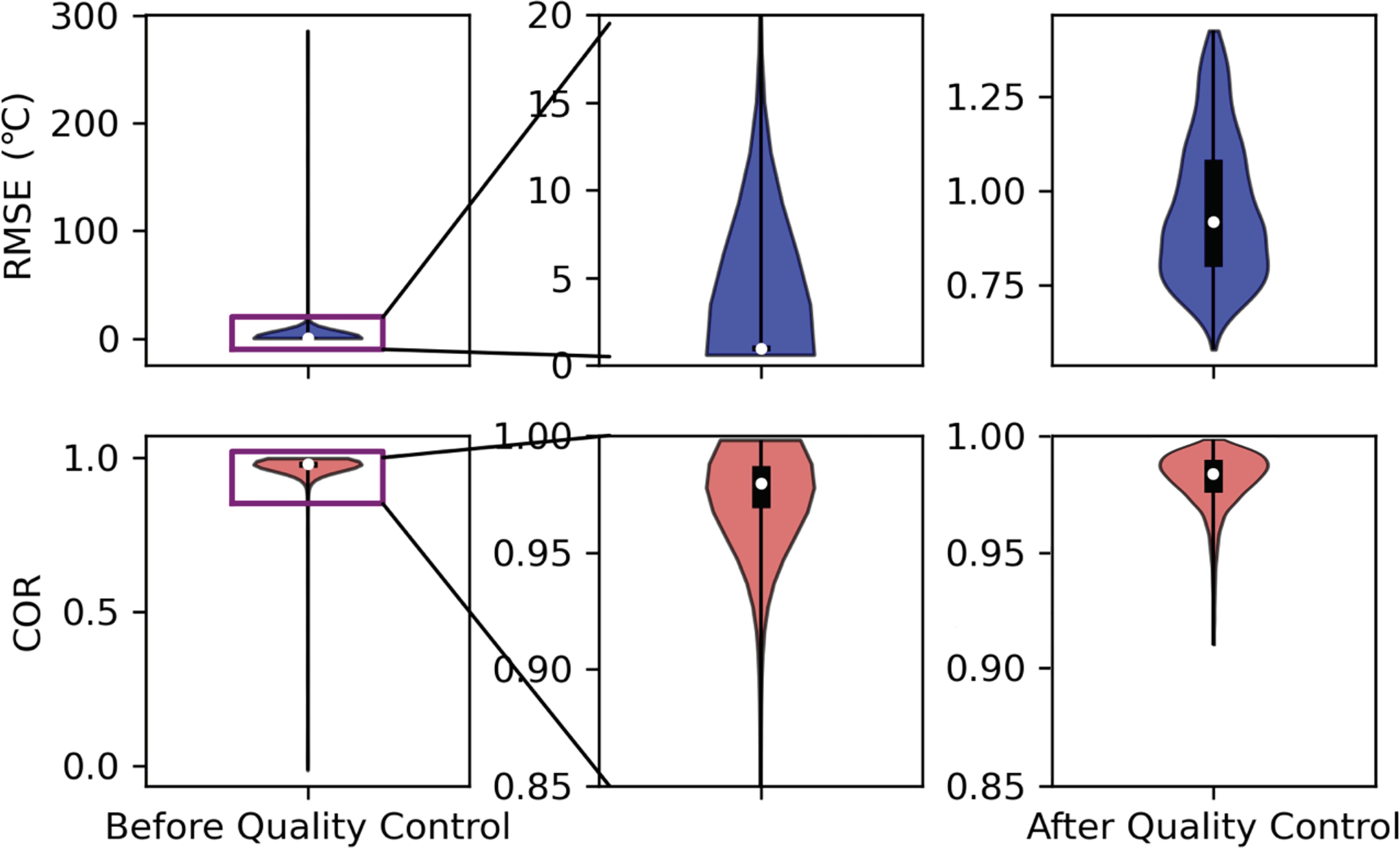
The effect of the entire database after quality control is shown in Fig. 3. We found that a large part of the RMSE of the data before quality control was greater than 5°C, and the COR was concentrated mainly above 0.9. After quality control, outliers can be eliminated, and the RMSE and COR then lie within a reasonable range.

Figure 3. A violin plot of the entire data set before and after quality control. After our effective quality control, most of the outliers have been eliminated.
-
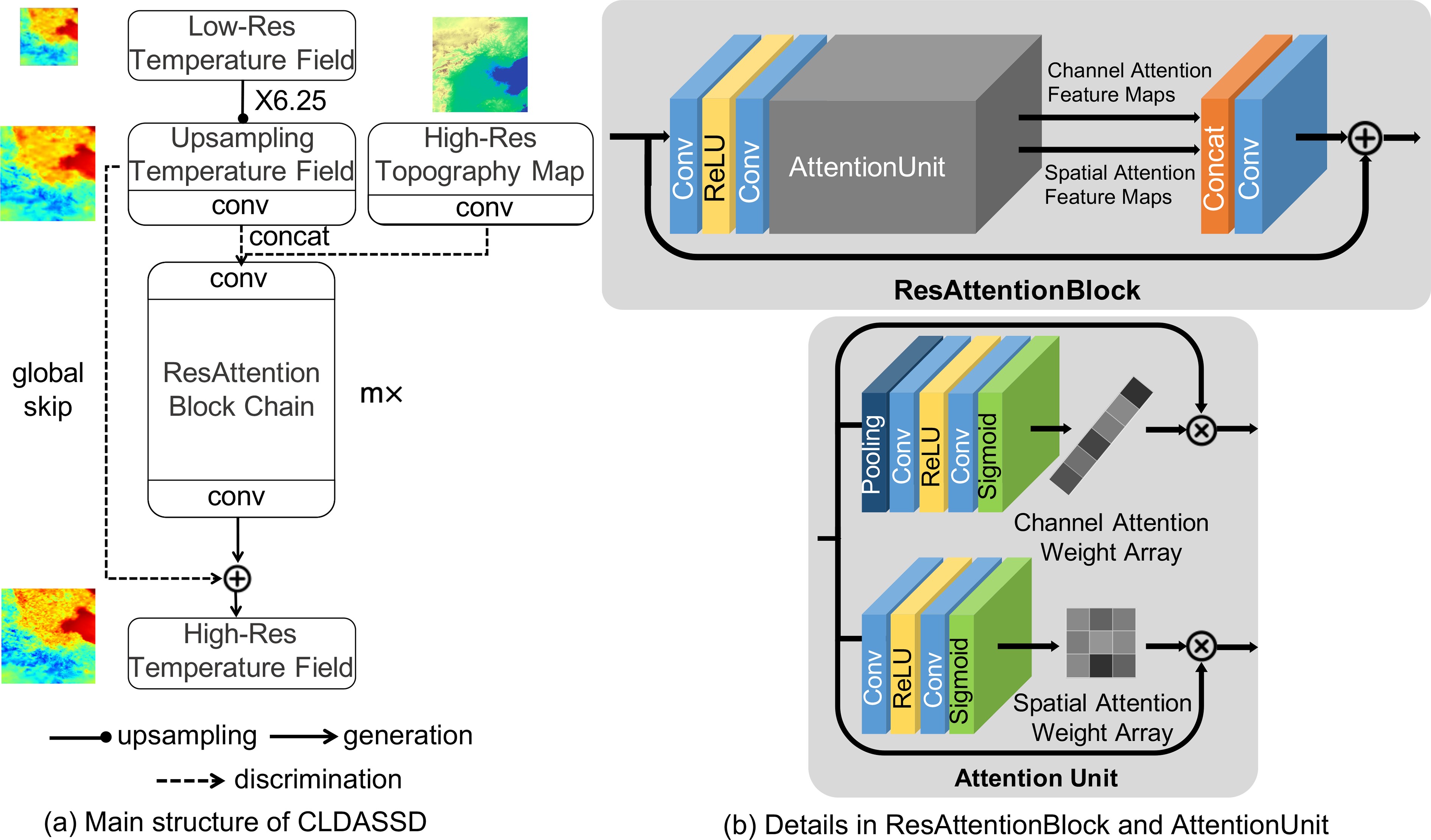
The backbone framework of our model uses VDSD (Mao, 2019). The very deep statistical downscaling model (VDSD) contains a large number of local skip connections. We have improved it, adding a global skip connection and attention mechanism, and call it the CLDAS Statistical Downscaling Model (CLDASSD). The input of CLDASSD is a coarse-resolution temperature field (0.0625° × 0.0625°) and fine-resolution DEM data (0.01° × 0.01°). After model training, the output is the temperature field magnified 6.25-fold (0.01° × 0.01°). CLDASSD mainly contains convolutional layers, pooling layers, rectified linear unit layers (ReLU), and sigmoid layers. The overall model design is shown in Fig. 4.
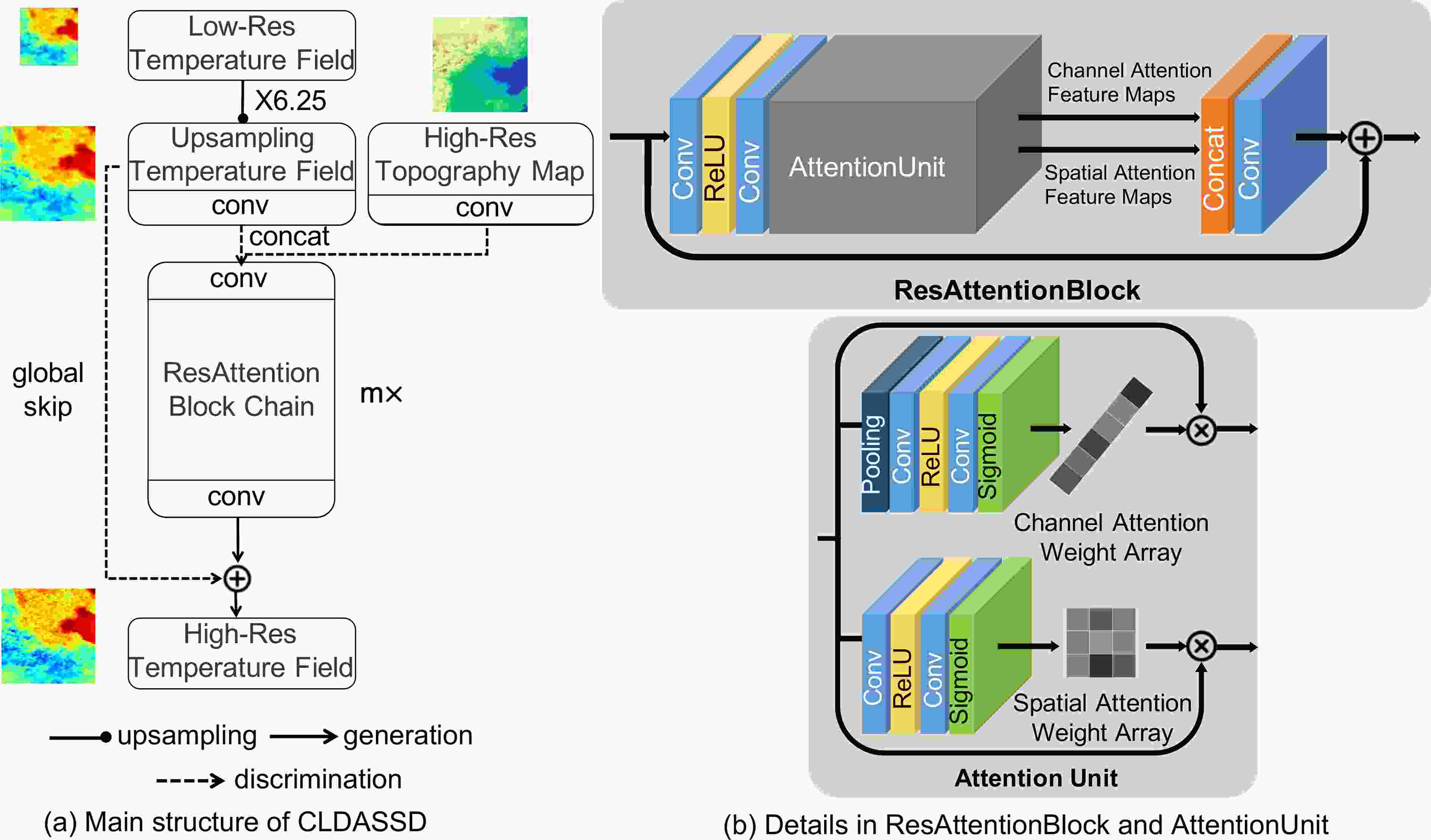
Figure 4. The design framework of CLDASSD. (a) shows the overall structure of the model; (b) shows the specific design details of the model's attention unit.
-
CLDASSD follows the pre-sampling structure of SRCNN (Dong et al., 2016), which locates the upsampling layer at the model's head. The upsampling method uses bicubic linear interpolation (Keys, 1981), within which we do not need to manually set any parameters for the models with different scale factors, which improves the model reusability. Furthermore, this approach can avoid the adverse effects of some learnable upsampling methods, such as a checkerboard effect from transposed convolution (Odena et al., 2016).
-
Suppose the model is
$ \mathcal{F}\left(*\right) $ , the input low-resolution temperature field denotes$ {T}_{\mathrm{c}\mathrm{o}\mathrm{a}\mathrm{r}\mathrm{s}\mathrm{e}} $ , the high-resolution DEM denotes$ H $ , and the output high-resolution temperature field denotes$ {T}_{\mathrm{f}\mathrm{i}\mathrm{n}\mathrm{e}} $ ; then,Here,
$ x $ is the residual error between the high- and low-resolution fields following the Gaussian distribution. The model fits a sparse Gaussian distribution, which is much easier than directly learning the mapping from low-resolution fields to high-resolution fields (Drozdzal et al., 2016). This connection method is widely used in single-image super-resolution (Kim et al., 2016; Tai et al., 2017a, b; Ahn et al., 2018).Therefore, we directly add the low-resolution field after the upsampling layer to the end of the model in CLDASSD (see Fig. 4a), which avoids learning the mapping of the entire temperature field to the entire temperature field and dramatically reduces the difficulty of model learning.
-
Our motive for using the attention mechanism is to be able to anticipate that the model can effectively extract critical information and suppress useless information during the training process. The design inspiration of CLDASSD is influenced by a channel-wise and spatial feature modulation network (CSFM, Hu et al., 2020), so we add an attention unit at the end of the standard residual structure.
The details of the attention unit are shown in Fig. 4b. We call the residual structure containing the attention unit ResAttentionBlock. The attention unit of each ResAttentionBlock contains two branches: a channel attention branch and a spatial attention branch. The spatial attention branch is used for pixel-level feature map processing: a two-dimensional weight vector can be obtained to suppress the low contribution area on each feature map. The channel attention branch is used to perform channel-level feature map processing: a one-dimensional weight vector can be obtained, and the feature map with a low contribution is directly assigned a lower weight. ResAttentionBlock then fuses the feature maps of the two branches after attention weight processing.
-
The formula for the vanilla L1 loss and its derivative is
$ {\mathcal{L}}_{\mathrm{L}1} $ is not derivable at 0. However, when the model fits the residual mentioned in section 3.2.1, there will be many zero values in the residual spatial distribution, making the model's output unstable. Therefore, we use Charbonnier loss (Lai et al., 2017), a kind of improved vanilla L1 loss, to serve as the model's loss function. The formula iswhere
$ {O}_{i} $ denotes the model output grid i,$ {G}_{i} $ denotes the HRCLDAS data grid i, and$ n $ denotes the number of grids.$ \epsilon $ is a constant, generally set to$ {10}^{-3} $ . This improvement makes the loss function derivable everywhere, and the model training process is more stable than with the vanilla L1 loss. -
CLDASSD is built on TensorFlow 1.4, and the entire model is trained on one NVIDIA 2080ti GPU. All convolution structures in the model use a convolution kernel with a size of 3 × 3 and a step size of 1 and perform Gaussian initialization; padding technology is used to ensure that all feature maps in the data stream maintain their shape. The number of ResAttentionBlocks, mx, means that there are m blocks (see Fig. 4a). In these paper m is 9, and the training batch size is 64 (these parameters are adjusted repeatedly). The Adam optimizer is used, and the learning rate is set to 0.001 to optimize the network model's parameters.
-
To evaluate the results of CLDASSD in detail and comprehensively, we design the "double true values" evaluation. Specifically, first, we use the observation data as the "true value" and take bias, root mean square error (RMSE), mean absolute error (MAE), and COR as metrics to evaluate the reconstruction field of the model. Moreover, we also care about the spatial distribution of the model’s reconstruction field and the accuracy of the texture details at high resolution. Therefore, we take HRCLDAS as the “true value” and use the peak signal-to-noise ratio (PSNR) and structural similarity (SSIM), which are often used in super-resolution, to evaluate the similarity between the reconstruction field and HRCLDAS.
Bias, RMSE, MAE, and COR are used mainly to evaluate the reconstruction field's pixel-level error. Their formulas are as follows:
where
$ {O}_{i} $ denotes the observations at weather station$ i $ (i.e., the true value),$ {G}_{i} $ denotes the reconstruction field interpolated to the corresponding station$ i $ , and$ N $ denotes the number of stations.For spatial distribution evaluation of the model downscaling results, we use PSNR and SSIM (Wang et al., 2004). The formulas are as follows:
$ {I}_{\mathrm{m}\mathrm{a}\mathrm{x}} $ refers to the bit depth of the data, and the value of$ {I}_{\mathrm{m}\mathrm{a}\mathrm{x}} $ is 255 for the natural image uint8 data type. Therefore, when calculating the PSNR of the temperature field, we convert the data range to (0, 255) so that$ {I}_{\mathrm{m}\mathrm{a}\mathrm{x}} $ can be calculated as 255.In Eq. (10),
$ {\mu }_{G} $ is the mean value of the reconstruction field,$ {\mu }_{O} $ is the mean value of the real high-resolution field (i.e., the second “true value,” the data from HRCLDAS),$ {\mathrm{\sigma }}_{\mathrm{G}} $ is the standard deviation of the reconstruction field,$ {\sigma }_{O} $ is the standard deviation of the real high-resolution field, and$ {\sigma }_{GO} $ is the covariance between the reconstruction field and the real high-resolution field.To compare with the results of CLDASSD, we use bilinear interpolation as the baseline for comparison experiments. The formula for bilinear interpolation is as follows:
$ Z\left({I}_{1},{J}_{1}\right) $ ,$ Z({I}_{1},{J}_{2}) $ ,$ Z\left({I}_{2},{J}_{1}\right) $ , and$ Z({I}_{2},{J}_{2}) $ are the variable values on the grid;$ Z\left({I}_{1},J\right)\;\mathrm{a}\mathrm{n}\mathrm{d}\;Z\left({I}_{2},J\right) $ are the interpolation results obtained after linear interpolation on the latitudes$ {I}_{1} $ and$ {I}_{2} $ , respectively; and$ Z\left(I,J\right) $ is the value at a specific position after interpolation.To illustrate the contribution of the attention mechanism and global skip connection proposed in this paper, we conduct a series of ablation experiments (sub-models) as shown in Table 1.
Model Structure CLDASSD_w The entire network has only a simple stack of residual structures. CLDASSD_a Based on the residual structure, we added the attention unit we designed. CLDASSD_g Based on CLDASSD_w, a global skip connection is added. CLDASSD This model has both a global skip connection and an attention mechanism. Table 1. Design framework of several ablation experiments (sub-models). It is used to evaluate the contribution of global skip connection and attention mechanism.
-
In the following results and discussion, it is assumed that the evaluation metrics results are all in the test set if no specific explanation is given. Except for PSNR and SSIM, we take the products from HRCLDAS as the “true value”; other metrics take site observation data as the “true value.”
First, the average of the evaluation metrics on the test set is given in Table 2. Compared with bilinear interpolation, our model provides an improvement, especially the improvement of SSIM by approximately 0.2. The apparent improvement of the visual evaluation metric, SSIM, can preliminarily illustrate the great potential of CLDASSD in estimating the structural features of high-resolution temperature fields.
Metrics Bilinear CLDASSD_w CLDASSD_a CLDASSD_g CLDASSD RMSE 1.37 1.34 1.34 1.31 1.30 MAE 0.97 0.95 0.95 0.94 0.93 PSNR 29.90 30.68 30.81 31.06 31.21 SSIM 0.35 0.57 0.59 0.59 0.60 Table 2. The average statistics for each metric in the test set (bold stands for the best). It can be seen that there is an improvement in SSIM.
To explore the model’s ability to reconstruct the temperature field under different types of terrain, we divide the DEM maps of the research area into an 8 × 8 chessboard, i.e., 64 small, uniform patches; the ID of each small patch is shown in Fig. 5. Then, we classify each patch into one of four terrain types (plain, water body, mountain, and plateau). Table 3 shows the specific content of each terrain set. Table 4 shows the evaluation results under the four terrain types. Compared with bilinear interpolation, CLDASSD provides a more substantial improvement in mountain areas, where the RMSE can be reduced by approximately 0.1°C, and a small improvement in plain, water body, and plateau areas. These results show that CLDASSD is particularly outstanding in reconstructing areas with complex terrain gradients. The remainder of this section will combine daily and seasonal change to evaluate the performance of CLDASSD.
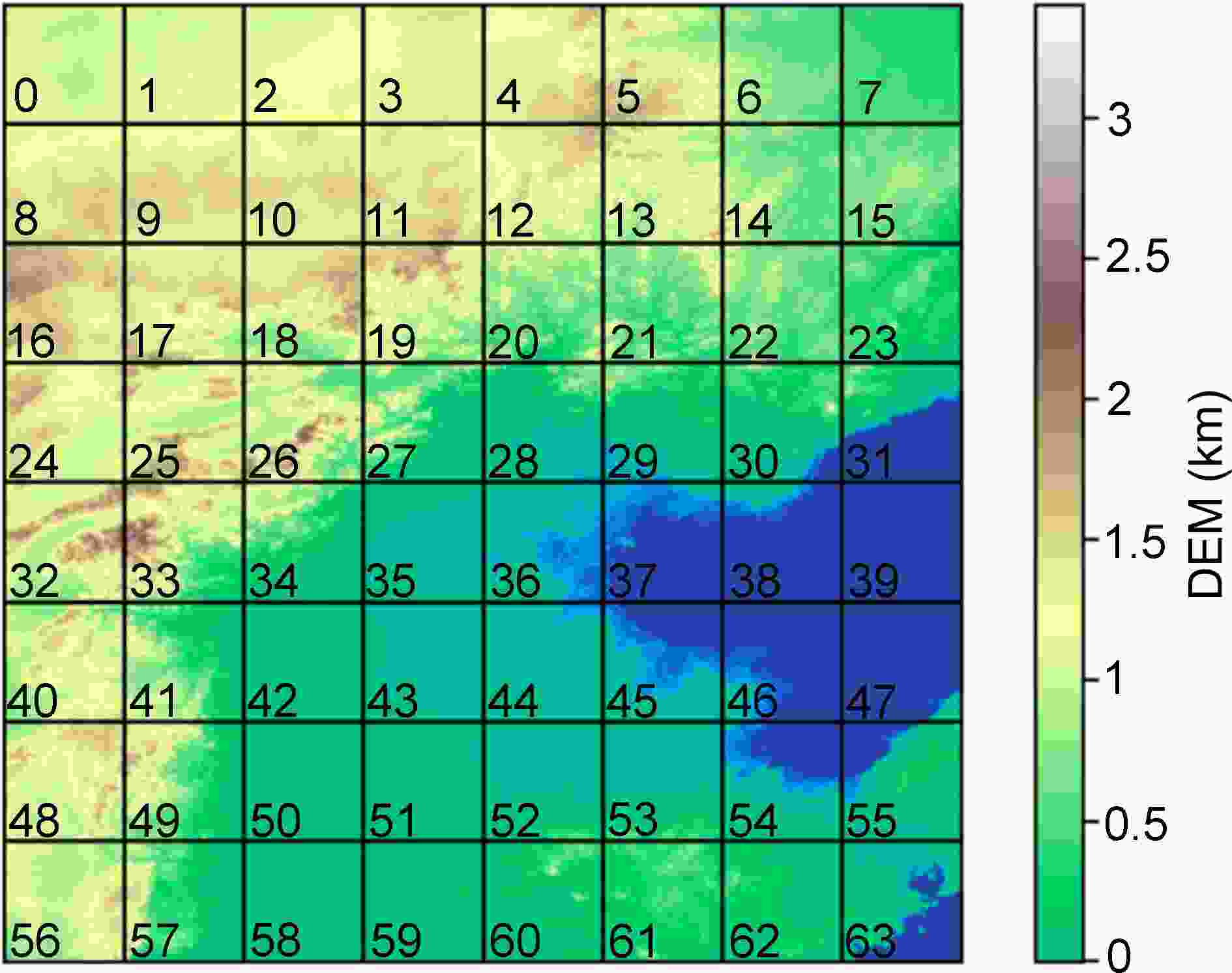
Figure 5. DEM map of the Beijing-Tianjin-Hebei region. We divided it into an 8 × 8 chessboard and assigned an ID to each patch.
Terrain type Set Mountain {5, 12, 13, 18, 19, 20, 21, 22, 25, 26, 27, 32, 33, 34, 40, 41, 48, 49, 56, 57, 60, 61} Plain {6, 7, 14, 15, 23, 28, 29, 30, 35, 36, 42, 43, 44, 50, 51, 52, 53, 55, 58, 59} Water body {31, 37, 38, 39, 45, 46, 47, 54, 62, 63} Plateau {0, 1, 2, 3, 4, 8, 9, 10, 11, 16, 17, 24} Table 3. Classification of all the patches in Fig. 5. We divided them into four types, i.e., mountain, plain, water body, and plateau.
Metrics Type Bilinear CLDASSD_w CLDASSD_a CLDASSD_g CLDASSD RMSE Plain 1.01 1.01 1.01 1.0 0.99 Water body 1.19 1.18 1.19 1.19 1.17 Mountain 1.61 1.55 1.55 1.51 1.50 Plateau 1.35 1.33 1.33 1.33 1.32 MAE Plain 0.73 0.73 0.73 0.73 0.72 Water body 0.87 0.86 0.86 0.87 0.85 Mountain 1.16 1.13 1.13 1.1 1.11 Plateau 1.0 0.99 0.99 0.99 0.98 Table 4. The reconstruction field for each time was divided into four different terrain types mentioned in Table 3 for evaluation. Although the RMSE is the highest in the mountainous area, it has the biggest improvement compared with that in bilinear interpolation (bold stands for the best).
-
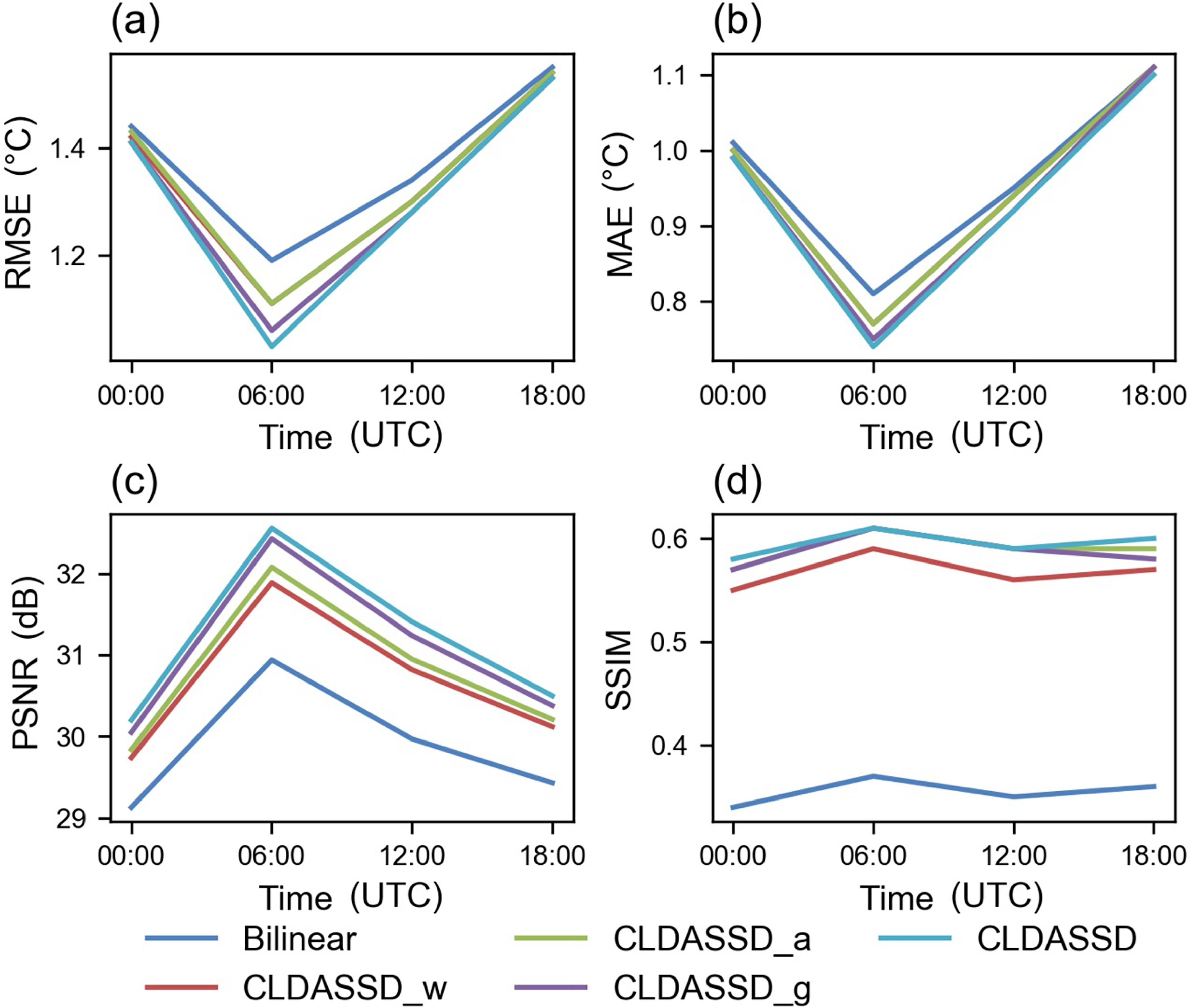
We evaluate the model according to different daily times (we use UTC times), and Fig. 6 shows the evaluation results. Figure 6a shows that the RMSE at 0600 UTC is the lowest, reduced by 0.13°C compared with that in bilinear interpolation. It is noteworthy that 0600 UTC occurs at noon in the local area when the spatial distribution of temperature has the strongest correlation with terrain elevation. As an auxiliary element, the terrain elevation data can provide more detailed information for the model at that time.

Figure 6. These four figures show the evaluation results of different metrics of different models in daily times (All times are coordinated universal time, UTC). (a), (b), (c), and (d) represent RMSE, MAE, PSNR and SSIM, respectively. CLDASSD performs best at 0600 UTC, i.e., noon in the local area.
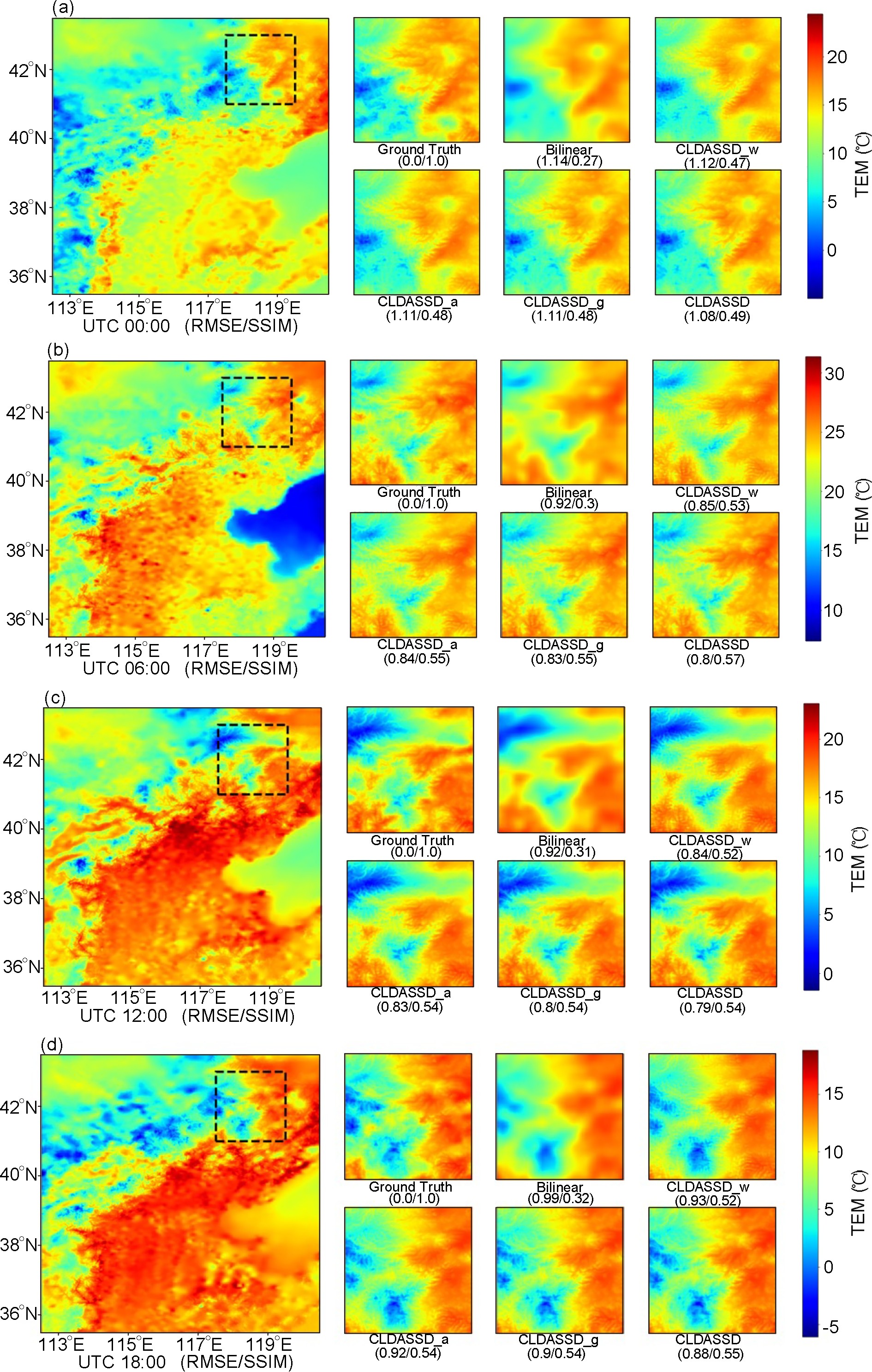
To evaluate the ability of CLDASSD to capture the spatial features of daily change in the temperature field, we use four daily times on 15 April 2019, as an example. Specific spatial details of the reconstruction are shown in Fig. 7. It can be seen that the spatial distribution of our model output is more similar to ground truth than that produced by bilinear interpolation (our models include CLDASSD and all sub-models). Specifically, our models have obvious advantages in the fine-scale reconstruction, noting that the output of bilinear interpolation is not detailed due to its averaging scheme. Our models also perform better in terms of metrics than bilinear interpolation in RMSE and SSIM; overall, CLDASSD is superior.
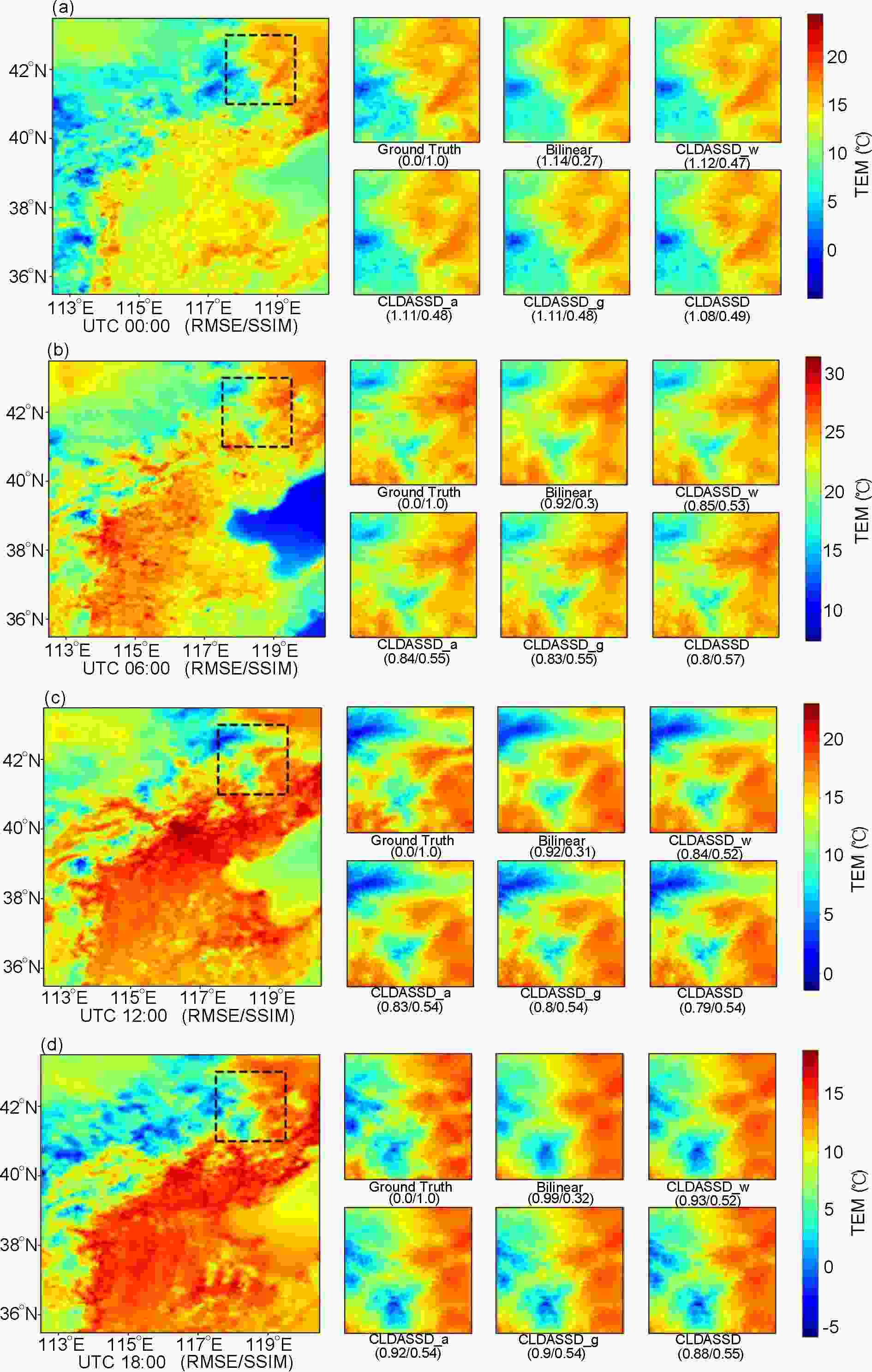
Figure 7. Analysis from 15 April 2019 used as an example to show the daily change of the spatial distribution of the temperature field in a fixed mountainous area (the area in the black box). (a), (b), (c), and (d) denote 0000, 0600, 1200, and 1800 UTC, respectively.
In summary, regardless of the visualization of spatial distribution or evaluation metrics, the reconstruction field of CLDASSD at each daily time is close to the “double true values,” which shows that CLDASSD has performance robustness regarding daily changes.
-
In this section, our models are re-evaluated according to season. The evaluation metrics results are shown in Fig. 8. Based on bilinear interpolation, CLDASSD has a similar improvement of RMSE for each season, with an average of approximately 0.07°C. Among the four seasons, the lowest RMSE is observed in summer, likely because the plains area is greatly affected by the summer monsoon. However, the plateau and mountainous areas are less affected by the summer monsoon. Thus, the temperature difference is most affected by terrain, and CLDASSD can make full use of the terrain’s data to reconstruct fine-scale details that are not observable in the coarse-scale temperature field. However, in winter (DJF), we found that the model fares much worse than in summer. The main reasons which explain this, center around the facts that the latent and sensible heat fluxes in winter are not as strong as in summer, and the spatial distribution of temperature is less affected by topography compared to summer. The auxiliary information input of our model only adds a DEM, resulting in poor results in winter. We also mention in section 4.3 that we will consider adding more factors that affect the spatial distribution of temperature in future work.

Figure 8. These four figures show the evaluation results of different metrics of different models in all seasons. (a), (b), (c), and (d) represent RMSE, MAE, PSNR, and SSIM, respectively. CLDASSD performs best in summer.
We select the seasonal representative day (the first of the month) at 0600 UTC, and the outputs of CLDASSD and bilinear interpolation are compared, as shown in Fig. 9. It can be found that in mountain and plateau areas, CLDASSD can estimate several subtle textures more accurately than bilinear interpolation. However, CLDASSD cannot evaluate small disturbances in the plains area, as can HRCLDAS products. Ground truth, bilinear interpolation, and CLDASSD are consistent in the water body, reflecting an insufficient improvement in water body representation.
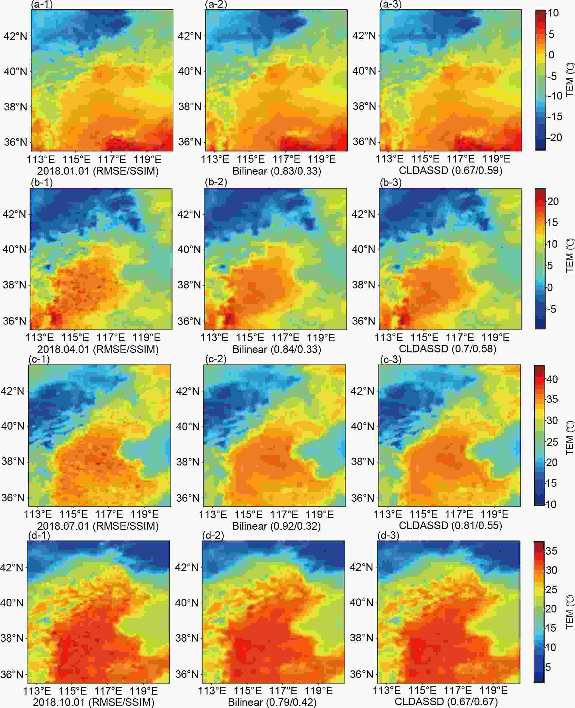
Figure 9. Analysis from the first day in each representative month of four seasons at 0600 UTC as an example to compare the seasonal change in reconstruction fields of bilinear interpolation and CLDASSD. The leftmost column is the product of HRCLDAS, the middle column is the output of bilinear interpolation, and the rightmost column is the output of CLDASSD. (a), (b), (c), and (d) denote the first day in January, April, July, October, respectively.
Reconstructing the subtle disturbances in the areas of the plains are not the primary task of our experiments. Such disturbances may arise from various physical processes. Moreover, for the plains area, the spatial gradient of the temperature field is not large, so ordinary interpolation methods can also reconstruct the fine-scale temperature field with very small error. However, temperature reconstruction for complex terrain requires the precise spatial distribution of temperature. Moreover, CLDASSD can estimate the fine texture of the temperature field, similar to HRCLDAS products, under complex terrain gradients. Moreover, from seasonal change, CLDASSD can reconstruct detailed textures in complex mountainous areas in every season. This robustness is similar to the robustness in daily change.
-
We have discussed the evaluation results according to daily times, seasons, and space. In terms of evaluation metrics and spatial distribution, CLDASSD has a lower RMSE than bilinear interpolation and can present finer-scale details.
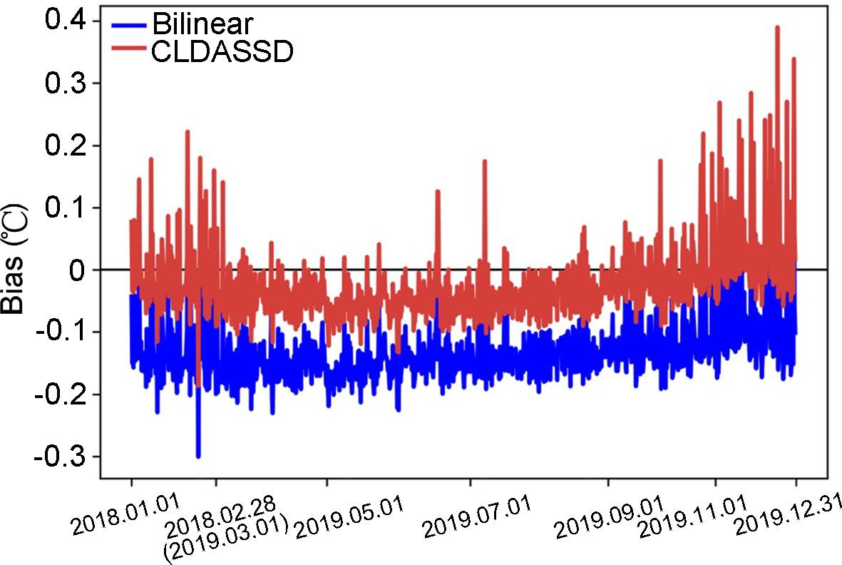
To further compare the output quality of CLDASSD and bilinear interpolation on the test set, it can be seen in Fig. 10 that the bias of bilinear interpolation is basically between –0.1°C and –0.2°C. Furthermore, CLDASSD has an improvement of approximately 0.1°C. In addition, the bias in summer is stable and close to zero, which echoes the previous analysis. We then determine the COR and RMSE frequency between the outputs of CLDASSD and bilinear interpolation, as shown in Fig. 11. The reconstructed field, with a COR greater than 0.98 and RMSE greater than 0.75°C, demonstrates an improvement.

Figure 10. The line chart of bias compares the bias of bilinear interpolation and CLDASSD on the test set. Because a different amount of data is discarded by quality control each month, the axis scale is not uniform.
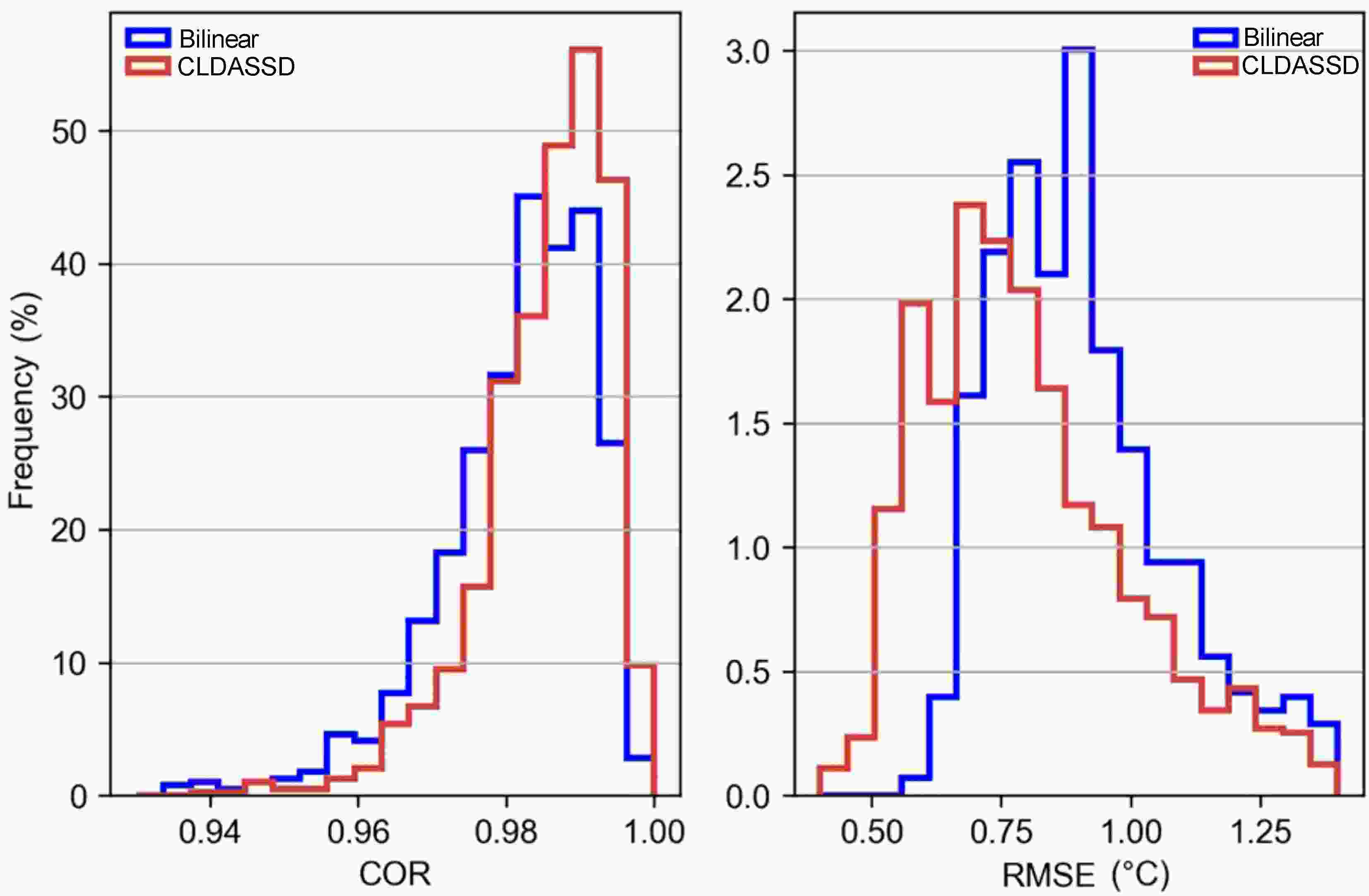
Figure 11. The frequency of COR and RMSE for bilinear interpolation and CLDASSD. It is clear that the output quality of CLDASSD is better than that of bilinear interpolation.
However, CLDASSD still has shortcomings. As discussed in section 4.2, CLDASSD performs only slightly better than bilinear interpolation in plains areas, but some subtle disturbances were absent or not well-simulated. This shortcoming is due to the small terrain gradient in plains areas, whereby the spatial distribution of temperature is less affected by the terrain. Therefore, in future work, we will select the underlying surface elements that influence the small disturbances in the plain areas, such as land cover, land utilization, ground incident solar radiation, and ground surface albedo. In addition, there is almost no improvement in the water area. This shortcoming may be due to the direct use of the same background field between CLDAS and HRCLDAS, precluding us from obtaining better results.
In addition to the above analysis of the advantages and disadvantages of the model results, we want to re-emphasize the advantages of the downscaling method based on deep learning in engineering. First, the deep learning model is a powerful feature extractor, which saves us from complicated feature engineering (e.g., accurately selecting sensitive factors related to temperature) during the data preparation phase. Second, many physical parameters need to be adjusted before running the test in a physical model, but the deep learning model only needs to adjust a few parameters that are independent of physics. Finally, the biggest advantage of the deep learning model in downscaling tasks is that it saves considerable amounts of computing power (Reichstein et al., 2019). It only needs a few GPUs to complete our needs, which is especially useful when the research area is larger and the resolution is higher, because the time complexity of the physical model will increase exponentially.
Finally, the downscaling task involves complex physical processes, and our experimental results still have room for improvement. We also need to have a deeper understanding of the use of deep learning for downscaling, such as designing more suitable models for downscaling tasks.
-
To fill the vacancy of assimilation data from HRCLDAS caused by the lack of surface observation data before 2008, we have designed a model based on deep learning for a preliminary study of this problem.
First, we propose an effective quality control method to control the quality of the paired data from CLDAS and HRCLDAS within a time range from 2018 to 2019. Then, informed by the deep-learning-based super-resolution algorithm, we propose a new temperature field downscaling model, named CLDASSD. The design of this model considers the attention mechanism and the global skip connection. To test the downscaling ability of CLDASSD in a variety of terrain areas, we take the Beijing-Tianjin-Hebei region with multiple landforms as the research area. Moreover, we use the experimental data from 31 March 2018 to 28 February 2019, to train the model, and the remaining data are used for testing. Finally, the performance of CLDASSD is evaluated by the “double true values” scheme from the perspectives of daily change, seasonal change, and spatial distribution.
The comparison experiment results and the ablation experiments show that CLDASSD is far superior to bilinear interpolation in evaluation metrics and spatial distribution. CLDASSD can estimate finer-scale temperature field details, which are close to HRCLDAS 2-m temperature products. The performance of CLDASSD is superior, especially regarding complex terrain, because CLDASSD can effectively make use the terrain data, which can provide considerable information for downscaling the temperature field.
Our research reveals the effectiveness of using the deep learning-based super-resolution algorithm for temperature field downscaling tasks. As noted in the introduction, our work is a preliminary study, so CLDASSD has not been evaluated on historical data (before 2008). In future work, we will continue to improve CLDASSD and back-calculate the data prior to 2008.
Acknowledgements. We would like to thank the National Key Research and Development Program of China (Grant No. 2018YFC1506604) and the National Natural Science Foundation of China (Grant No. 91437220) who supported this research.
| Model | Structure |
| CLDASSD_w | The entire network has only a simple stack of residual structures. |
| CLDASSD_a | Based on the residual structure, we added the attention unit we designed. |
| CLDASSD_g | Based on CLDASSD_w, a global skip connection is added. |
| CLDASSD | This model has both a global skip connection and an attention mechanism. |


 AAS Website
 AAS WeChat