


 DownLoad:


-
Zonda wind (Argentinian foehn) is a strong, warm, and very dry wind associated with adiabatic compression upon descending over the eastern slopes of the Andes Cordillera and occurs most often in winter and spring, mainly in the provinces of Mendoza and San Juan (Norte, 2015; Otero and Norte, 2015). Despite the constant improvement of numerical weather prediction (NWP) models and the advances in the understanding of mountain meteorology dynamics over the past decades, downslope windstorms forecasting is still limited by several factors. These factors include the dependency and sensitivity to the model’s resolution (e.g., Reinecke and Durran, 2009b; Jackson et al., 2013), numerical schemes, vertical coordinates and diffusion parametrizations (e.g., Smith, 2007), physical formulations (the boundary layer especially, see Smith, 2007), and initial condition uncertainties (e.g., Reinecke and Durran, 2009a). Thus, it is necessary to predict occurrence using statistical forecasting models specifically developed for these stations, which can improve or contribute to the NWP models.
In the 1960s, Widmer developed a “foehn test” for the Altdorf, Switzerland foehn station that was refined by Courvoisier and Gutermann (1971). This test remains as the operational tool used today. Later, Dürr (2008) developed an automated method for identifying foehn (i.e., nowcasting foehn). His procedure is based on 10-min real-time data from the automated Swiss surface network. Quite recently, Drechsel and Mayr (2008) developed an objective, probabilistic forecasting method for foehn in the Wipp Valley (Innsbruck) based on the ECMWF model output. In Sprenger et al. (2017), a new objective method for foehn prediction based on a machine learning algorithm (called AdaBoost, short for adaptive boosting) is proposed to distinguish between foehn and non-foehn events. Further improvement will require the use of not only deterministic, but also statistical methods. In particular, ongoing work shows that model output statistics (MOS) are a promising tool for improving foehn forecasting.
Considering the influence on the flow response when interacting with a topographic barrier, the development of the phenomenon is closely related to the vertical structure of the atmosphere, where mountain height, buoyancy frequency, and incident wind control the mountain waves activity and the dynamics of downslope wind (Durran, 1990; Smith and Skyllingstad, 2011; Damiens et al., 2018, among others). The application of statistical techniques, such as the study of Empirical Orthogonal Functions (EOF) or the Principal Component Analysis (PCA), allow the objective statistical characterization of vector and scalar variables or other physical variables, like temperature, humidity, wind, and stability. Otero et al. (2018) obtained an index for predicting the Zonda occurrence through the vertical sounding of the lee side of the Andes. A PCA is used to identify the patterns of the vertical structure of the atmosphere leading up to a Zonda wind event and used to construct the index model. A Zonda/non-Zonda index is calculable from T and Td profiles and is dependent on the climatological features of the region.
In the present work, the methodology of Otero et al. (2018) is followed. Here, a substantial improvement is presented with respect to the previous work, where only two combined leeward variables were used (temperature and dewpoint temperature). In this new version, not only are windward soundings (Chilean side) added, but so are new and different combinations between variables and soundings, combining up to four variables on each side of the Andes. The newly added variables are wind (U and V) and the squared Brunt–Väisälä frequency (N2), which are key factors in the atmospheric conditions for the development of this kind of downslope windstorm. Likewise, new metrics of the prediction model (not presented in Otero et al., 2018) are calculated such as the probability of detection (POD), probability of false detection (PODF), missing ratio (MR), false alarm rate (FAR), missing alarm ratio (MAR), and correct alarm ratio (CAR). In this case, the PCA is used to characterize the vertical structure on both sides of the Andes Mountains prior to the onset of a downslope windstorm (Zonda). A complete description of the vertical structure of wind, temperature, dewpoint, and stability for Zonda and non-Zonda events and the characteristic structure that discriminates between both classes are obtained.
The structure of this paper is as follows: Section 2 describes the data and methodology, where the PCA and index model are described. Section 3 presents the results including mean and Zonda soundings, the index model efficiency and metrics, and the discriminant sounding. Finally, the discussion and conclusions and their applications are presented in section 4.
-
For this study, available daily sounding data at 1200 UTC for the 1981–2019 period are taken for both sides of the Andes Mountains. The Santo Domingo surface station (33.65°S, 71.61°W, 75 m A. S. L.) on the Chilean side (Andes windward) and the Mendoza Airport surface station (32.83°S, 68.77°W, 704 m A. S. L.) on the Argentinean side (Andes lee side) are used (Fig. 1). The selected pressure levels for Mendoza´s soundings are those standard levels between 850 hPa and 300 hPa (i.e., 850, 700, 500, 400, and 300 hPa) and for Santo Domingo those between 1000 hPa and 200 hPa (i.e., 1000, 850, 700, 500, 400, 300 and 200 hPa). The sectioned levels are due to the vertical resolution of the vertical soundings of each side, those on the windward side having the highest vertical (as well as temporal) resolution, as well as the altitude of the locations. The selected variables are temperature (T), dewpoint temperature (Td), zonal (U) and meridional (V) wind components, and the squared Brunt–Väisälä frequency (N2). A data consistency is made by removing those inconsistent values. Missing data are detected and marked along with suspicious and out of range values, which is extremely challenging due to the event’s extreme nature.

Figure 1. (a) South America region with topographic height (shading, units: m) and (b) zoomed-in region over surface weather stations. Black dots and white line correspond to sounding stations and filled black dots correspond to the stations used for Zonda wind classification.
-
The Zonda wind classification is made using hourly data from three surface stations on the lee side (Fig. 1, black dots) belonging to the National Weather Service of Argentina (SMN): Mendoza Airport, Mendoza Observatory (32.9°S, 68.866°W, 827 m A. S. L.), and San Juan Airport (31.56°S, 68.5°W, 598 m A. S. L.). The predictor variables are temperature (T), dewpoint temperature (Td), surface pressure (P), and 10-m wind speed (V). The surface stations report hourly and have data records of 35 years for Mendoza Airport, 24 years for San Juan Airport, and 13 years for Mendoza Observatory. This classification is made manually (subjective) according to an abrupt increase in temperature and decrease in dewpoint temperature in conjunction with an increase in wind speed.
Figure 2a shows the Zonda climatology for the three surface stations and for the sounding data. Note that the Zonda wind presents higher frequencies of occurrence in winter and spring (mainly from June to October). The soundings used in this work must meet the requirements of section 2.1, in addition to having soundings on both sides of the Andes on the same day. This implies a total of 58 soundings (previous to the onset of the events) that presents the maximum frequency in October. The duration of Zonda events shows maximum frequencies between two to eight hours for Mendoza’s station and longer for San Juan Airport (Fig. 2b). The onset time presents highest frequencies in the afternoon, from 1500 UTC to 2100 UTC during winter, and a second maximum between 0000 UTC to 0300 UTC in spring (Fig. 2c).
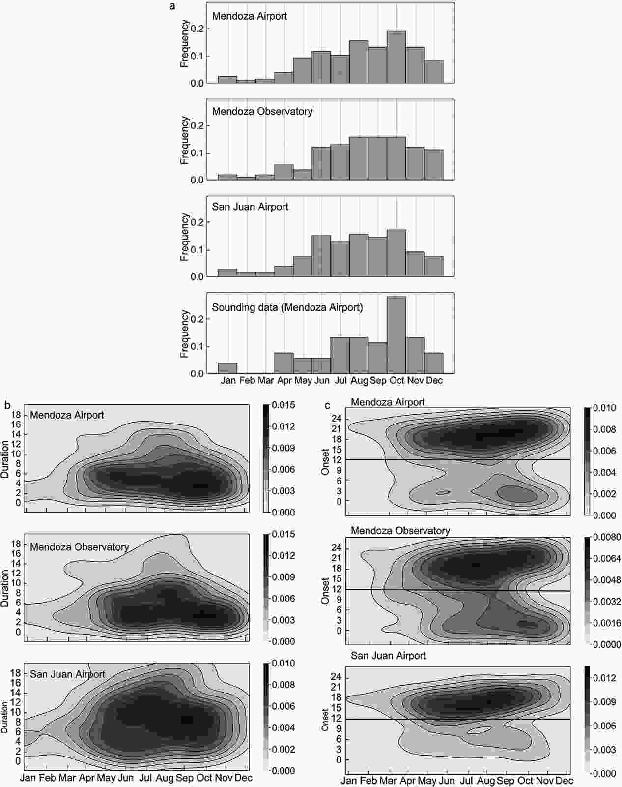
Figure 2. (a) Zonda events distribution for the surface stations and for sounding data used. (b) Zonda duration annual frequency distribution. (c) Zonda onset time annual frequency distribution. The straight line corresponds to the sounding hour (1200 UTC).
Once all Zonda events and their onset times have been found, the sounding data series is constructed. For this, the 1200 UTC sounding closest to the onset time of each event is considered (according to the onset time frequency, the 1200 UTC sounding is more likely to be closer to the event than the 0000 UTC sounding, and at the Mendoza Airport, no sounding for 0000 UTC is carried out, at least in a large part of the record). For example, if the event starts at 1500 UTC, the 1200 UTC sounding on the same day is considered (i.e., three hours after the event). If the event starts at 0900 UTC, the 1200 UTC sounding of the previous day is considered (i.e., 21 hours after the event). It is in this way that these soundings represent the characteristics of the atmosphere prior to the development of the Zonda wind.
The selection of the days without Zonda is done in such a way that the closest Zonda day is at least five days away. In this way, it is ensured that the synoptic conditions are as different as possible from those of a Zonda day. Data from a total of 116 soundings associated with Zonda and non-Zonda events are chosen to perform the PCA. This dataset is the same used in Otero and Araneo (2021).
-
The methodology for the PCA follows that used in Araneo et al. (2011) and Otero et al. (2018). The Zonda/non-Zonda probability index is obtained from a logistic regression between the PCA loading components and a vector of 0 and 1, associated with Zonda/non-Zonda. To detect the patterns capable of discriminating between Zonda and non-Zonda cases, they must first be compared with random non-Zonda conditions. The selection of those dates is carefully made so that they are not close to any Zonda events. As a necessary condition, it is considered that these days are at least five days away from any Zonda events.
For the calculation of the PCA, the sounding data are arranged forming a matrix
${\left[\boldsymbol{X}\right]}_{5\times 116}$ ($[{\boldsymbol{X}]}_{5\times 116}$ is a matrix of size 5 × 116) in which the rows contain the values corresponding to each pressure level for the variable to evaluate (T, Td, U, V, or N2), and each column represents the sounding for a given day. After that, the mean sounding is removed, obtaining the deviations matrix${\tilde{\left[{{\boldsymbol{X}}}\right]}}_{5\times 116}$ . This matrix is then standardized by columns. Of the 116 days, half correspond to Zonda soundings, and the other half correspond to non-Zonda soundings. In the case of Santo Domingo, the matrix has dimensions of [7 × 116] because more vertical levels are considered.The probability model (index) is built with the fit coefficients of a logistic regression for a binomial function. So, the logistic regression is transformed into probability values between 0 and 1. Then, for the ith element, the probability will be given by:
where
$ {w}_{i} $ is the ith element of$\boldsymbol{w}={{b}_{0}+b}_{1}{\boldsymbol{f}}_{1}+{b}_{2}{\boldsymbol{f}}_{2}+\dots $ $ +{b}_{n}{\boldsymbol{f}}_{n}$ ,${\boldsymbol{f}}_{1},{\boldsymbol{f}}_{2}, \dots ,{\boldsymbol{f}}_{n}$ are the principal component loadings (columns of F),$ {b}_{0},{b}_{1},\dots \dots ,{b}_{n} $ are the regression coefficients (fitted with the maximum likelihood method), and$ n $ is the number of significant components retained. Then,$ {\widehat{c}}_{i} $ is an estimator of the ith coefficient of$ \mathit{c} $ (known vector of zeros and ones, associated with Zonda/non-Zonda events) corresponding to the ith day. This estimator represents the probability that day has of being classified as Zonda or non-Zonda based on a preset cutoff threshold of the index.The component loadings matrix can be written as
$\boldsymbol{F}={{\tilde{\boldsymbol{X}}}_{\mathrm{s}}}'{\boldsymbol{Z}}_{\mathrm{s}}/(m-1)$ where$ m $ is the number of rows (days) of$\boldsymbol{X}$ . So,$\boldsymbol{w}={{\tilde {\boldsymbol{X}}}_{\mathrm{s}}}'{{\boldsymbol{Z}}^{*}_{\mathrm{s}}}{\boldsymbol{b}}^{*}/(m-1)+{b}_{0}\left[1\right]$ where${{\boldsymbol{Z}}^{*}_{\mathrm{s}}}$ is the matrix containing the standardized score components corresponding to the predictor variables used in the model (i.e., all those components related to the significant fit coefficients$ {b}_{i} $ ),${\boldsymbol{b}}^{*}$ is the vector matrix containing the coefficients$ {b}_{0},{b}_{1},\dots \dots ,{b}_{n} $ , and [1] is a column vector of elements equal to 1.The vector
$\boldsymbol{A}={{\boldsymbol{Z}}^{*}_{\mathrm{s}}}{\boldsymbol{b}}^{*}/(m-1)$ only depends on the PCA results and the regression analysis. Once$\boldsymbol{A}$ and$ {b}_{0} $ are determined from the statistical analysis described, given any standardized anomaly sounding${\tilde {\boldsymbol{x}}}_{\mathrm{s}}$ (not necessarily belonging to this analysis), the Zonda/non-Zonda index can be estimated by the equation:where
$\hat{c}$ represents the Zonda wind occurrence probability, serving as a useful forecast tool for that particular day.In order to estimate prediction errors, the leave-one-out cross-validation method is implemented. In other words, for the construction of the Zonda index, all the dates except one are used in each step, which is used for its verification. Thus, in each step, the set formed by
$ n-1 $ observations is considered the fitting set. The observation which is left out is then used to test the regression model obtained with the remaining ones. This procedure is performed with each date, obtaining a verification for each particular date.This procedure can be generalized using all the predictor variables in a single prediction index to improve the efficiency of the forecast index. Suppose the case with 2 variables, in principle with the same number of cases
$ {n} $ ,${\boldsymbol{X}}_{1}$ and${\boldsymbol{X}}_{2}$ , with dimensions$ t $ and$ r $ , respectively. For example, suppose that we have$ n $ days,${\boldsymbol{X}}_{1}$ is the matrix containing the Mendoza station’s soundings for each day’s temperatures at$ t $ vertical levels, and${\boldsymbol{X}}_{2}$ is the matrix containing the Santo Domingo station’s soundings for each day’s squared Brunt–Väisälä frequency at$ r $ vertical levels; then:From a separate PCA for each variable, the components of each variable
$ {\boldsymbol{Z}}_{{s}_{1}} $ and$ {\boldsymbol{Z}}_{{s}_{2}} $ are obtained. Neglecting the non-significant components of each PCA (suppose$ {d}_{1} $ and$ {d}_{2} $ components, respectively), the significant standardized score components are${{\boldsymbol{Z}}^{*}_{{s}_{1}}}={\left[{{\boldsymbol{Z}}^{*}_{{s}_{1}}}\right]}_{t\times (n-{d}_{1})}$ and${{\boldsymbol{Z}}^{*}_{{s}_{2}}}= $ $ {\left[{{\boldsymbol{Z}}^{*}_{{s}_{2}}}\right]}_{r\times (n-{d}_{2})}$ , and the associated matrices of eigenvectors and eigenvalues are${{\boldsymbol{Q}}^{*}_{1}}={\left[{{\boldsymbol{Q}}^{*}_{1}}\right]}_{n\times (n-{d}_{1})}$ ,${{\boldsymbol{Q}}^{*}_{2}}={\left[{{\boldsymbol{Q}}_{2}}^{*}\right]}_{n\times (n-{d}_{2})}$ ,${{\boldsymbol{D}}^{*}_{1}}={\left[{{\boldsymbol{D}}^{*}_{1}}\right]}_{n\times (n-{d}_{1})}$ , and${{\boldsymbol{D}}^{*}_{2}}={\left[{{\boldsymbol{D}}^{*}_{2}}\right]}_{n\times (n-{d}_{2})}$ . With these matrices as a whole, the logistic regression is carried out, correlating the$ \boldsymbol{c} $ vector with the joint matrix$\tilde {\boldsymbol{Q}}= $ $ {\left({{\boldsymbol{Q}}^{*}_{1}}|{{\boldsymbol{Q}}^{*}_{2}}\right)}_{n\times (2n-{d}_{1}-{d}_{2})}$ from which the regression coefficients$\boldsymbol{b}={\left[{\boldsymbol{b}}\right]}_{(2n-{d}_{1}-{d}_{2})\times 1}$ are obtained, where$ {b}_{0} $ is the independent coefficient, the following$ {b}_{1},\dots \dots ,{b}_{n-{d}_{1}} $ correspond to the first variable$ {\boldsymbol{X}}_{1} $ (Temperature for Mendoza’s sounding), and the following$ {b}_{n-{d}_{1}+1},\dots \dots ,{b}_{n-{d}_{2}} $ correspond to the second variable$ {\boldsymbol{X}}_{2} $ (squared Brunt–Väisälä frequency for Santo Domingo’s sounding). With this data, the matrices$ {\left[{\boldsymbol{A}}_{1}\right]}_{t\times 1} $ and$ {\left[{\boldsymbol{A}}_{2}\right]}_{r\times 1} $ are calculated as:where
${\boldsymbol{b}}_{1}$ and${\boldsymbol{b}}_{2}$ are the column vectors formed by the coefficients$ {b}_{1},\dots \dots ,{b}_{n-{d}_{1}} $ and$ {b}_{n-{d}_{1}+1},\dots \dots ,{b}_{n-{d}_{2}} $ , respectively. Finally, the joint index for these variables is obtained as:Note that
${\left[{\boldsymbol{A}}_{1}\right]}_{t\times 1}$ and${\left[{\boldsymbol{A}}_{2}\right]}_{r\times 1}$ have the same dimensions of the predictor variable (i.e., number of vertical levels of Mendoza and Santo Domingo’s soundings, respectively) and that the$ \widehat{c} $ value depends on the dot product with the particular variable of the day to forecast. The value of$ \widehat{c} $ will be closer to 1 as the larger the scalar products between the particular variables and the vectors$\boldsymbol{A}$ with a positive sign, and it will be closer to 0 as less the smaller the scalar products with a negative sign be. Therefore, the$\boldsymbol{A}$ vectors can be interpreted as a "discriminant" vertical sounding of Zonda or non-Zonda situations. -
To compare among the models and the predictive skills of each one, different metrics, obtained from the confusion matrix, are used following the corrigendum of Barnes et al. (2007) (Tables 1 and 2).
Predicted Yes (Zonda) No (non-Zonda) Observed (Zonda) TP FN (Hit Zonda) (surprise) No event (non-Zonda) FP TN (Zonda False Alarm) (Hit non-Zonda) Table 1. Contingency table. TP (true positives), FP (false positives), FN (false negatives), and TN (true negatives).
Expression Description POD TP/(TP+FN) Probability Of Detection (event-based) MR FN/(TP+FN) = 1−POD Miss Ratio (event-based) CAR TP/(TP+FP) Correct Alarm Ratio (alarm-based) FAR FP/(TP+FP) = 1−CAR False Alarm Ratio (alarm-based) POFD FP/(TN+FP) Probability Of False Detection (event-based) MAR FN/(TN+FN) Missed Alarm Ratio (alarm-based) Table 2. Description of metrics used for the validation of the model.
-
The objective of this work is to detect those vertical profiles that may be able to detect the development of a Zonda event. For the statistical analysis (i.e., PCA), soundings anomalies with respect to the mean sounding of each station are used.
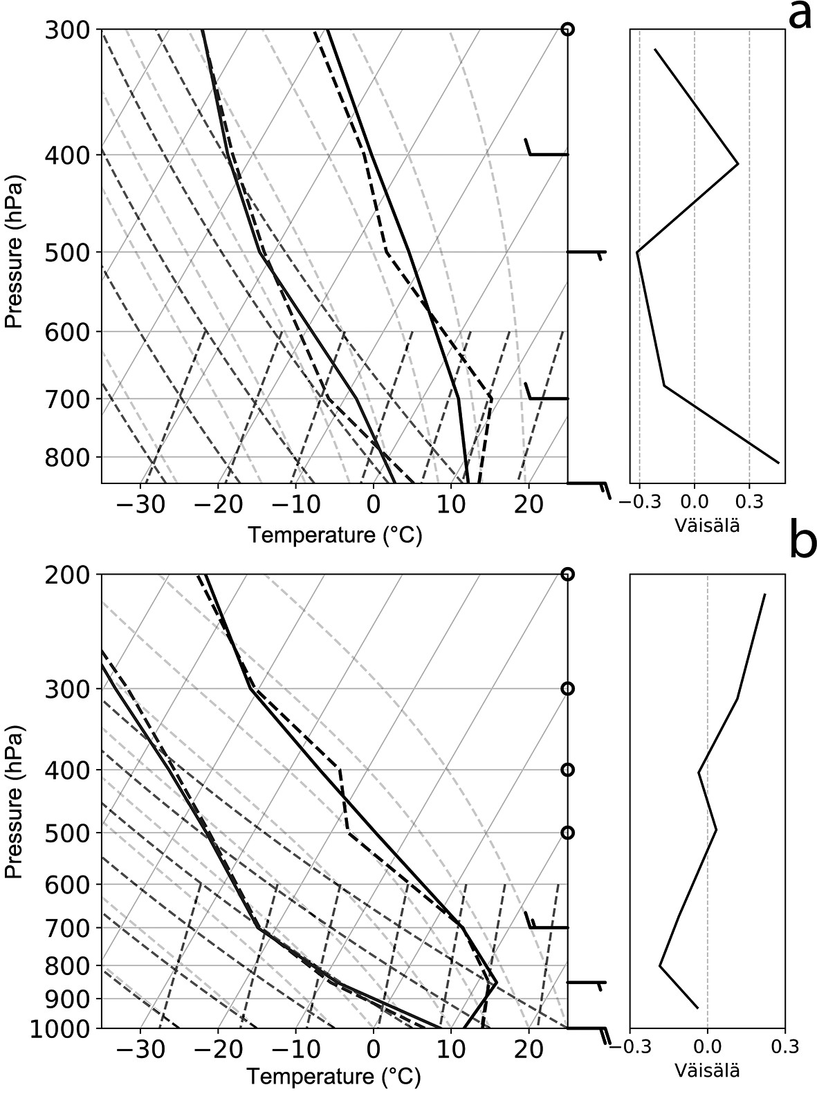
Figure 3a shows Mendoza’s mean sounding (full line) and the mean sounding for Zonda events on a skew-T diagram. The mean sounding is a statically stable profile throughout the vertical. The vertical profile associated with Zonda is also stable, but in this case, it is less stable (than the mean sounding) due to the lower levels warming. Dry conditions throughout the profile are observed, with a dew point depression of approximately 10°C and higher at midlevels. Surface winds are weak up to 700 hPa from a northwest direction, rotating to the west with a maximum of 45 kt (knot; where 1 kt = 0.51 m s−1) at 300 hPa. The mean sounding associated with Zonda events shows positive temperature anomalies from 850 hPa up to 600 hPa in conjunction with negative dewpoint anomalies, with a maximum dewpoint depression at 700 hPa. Above 500 hPa (approximately the height of the orographic barrier), there are no significant differences with the mean sounding, other than small negative temperature anomalies in the Zonda soundings. Positive wind anomalies are observed from 700 hPa to upper levels. The observed speeds are generally greater than mean conditions, exceeding 60 kt at 300 hPa, while directions are almost the same as in the mean sounding.

Figure 3. (a) Mean (solid line) and Zonda (dotted line) vertical soundings at 1200 UTC for Mendoza Airport and (b) Santo Domingo (right). Wind barbs on the left correspond to the Zonda sounding, and wind barbs on the right correspond to the mean sounding.
The Santo Domingo station’s mean sounding presents a vertical profile with a quasi-isothermal layer between 1000 hPa and 850 hPa, mainly associated with subsidence due to the presence of the Semipermanent Pacific Anticyclone (Fig. 3b). Near-surface winds are weak and rotating to the NW at 700 hPa with a maximum speed of 60 kt at 200 hPa. The vertical windward profile associated with Zonda events presents a relatively wetter and colder environment throughout the vertical. The surface layer is less stable and the winds are more intense, with values of 45 kt at 500 hPa and a maximum of 95 kt at 200 hPa. The windward mid and upper level winds are greater than those observed on the lee side, indicating the incidence of the mountain waves (Durran, 1990).
-
The PCA is primarily used as an exploratory tool in data analysis and for making predictive models. In this work, this analysis is used to characterize the vertical structure of the atmosphere on both sides of the Andes Mountains previous to a Zonda wind event. Also, by implementing a multiple logistic regression model for a binomial function between the response vector
$ \mathit{c} $ and the loadings components${\boldsymbol{f}}_{j}$ , a probability index of Zonda occurrence is defined (probabilistic predictive model) as shown in the methodology.For the PCA and the index construction, 116 soundings from the Mendoza and Santo Domingo stations at 1200 UTC are taken, constructing the anomaly matrix for the selected variables and levels. Half of these soundings correspond to Zonda wind events and the other half to random dates, where the presence of Zonda was not recorded (see their selection in methodologies). To obtain the index, an iteration is carried out in the PCA, with 115 soundings and leaving 1 out to evaluate the efficiency of the model for each cut-off value of the index. This procedure is carried out for each date, obtaining the Principal Components (
$\boldsymbol{F}$ ), the regression coefficients ($ {b}_{0},{b}_{1},\dots \dots ,{b}_{n} $ , related to the predictors used in the regression), the discriminant sounding ($\boldsymbol{A}$ vector, see section 2.2.3), the standardized score components (${{\boldsymbol{Z}}^{*}_{\mathrm{s}}}$ ), and the eigenvalues ($\boldsymbol{D}$ ) and eigenvectors ($\boldsymbol{Q}$ ).After performing the PCA, an index value is obtained for each date. Taking into account that the Zonda and non-Zonda events are known in advance, the obtained index values for each date are assigned to each class, and their distribution is analyzed. The model efficiency depends on the selected cut-off value of the index. Let’s firstly consider the model for the Mendoza soundings (lee side) for temperature.
-
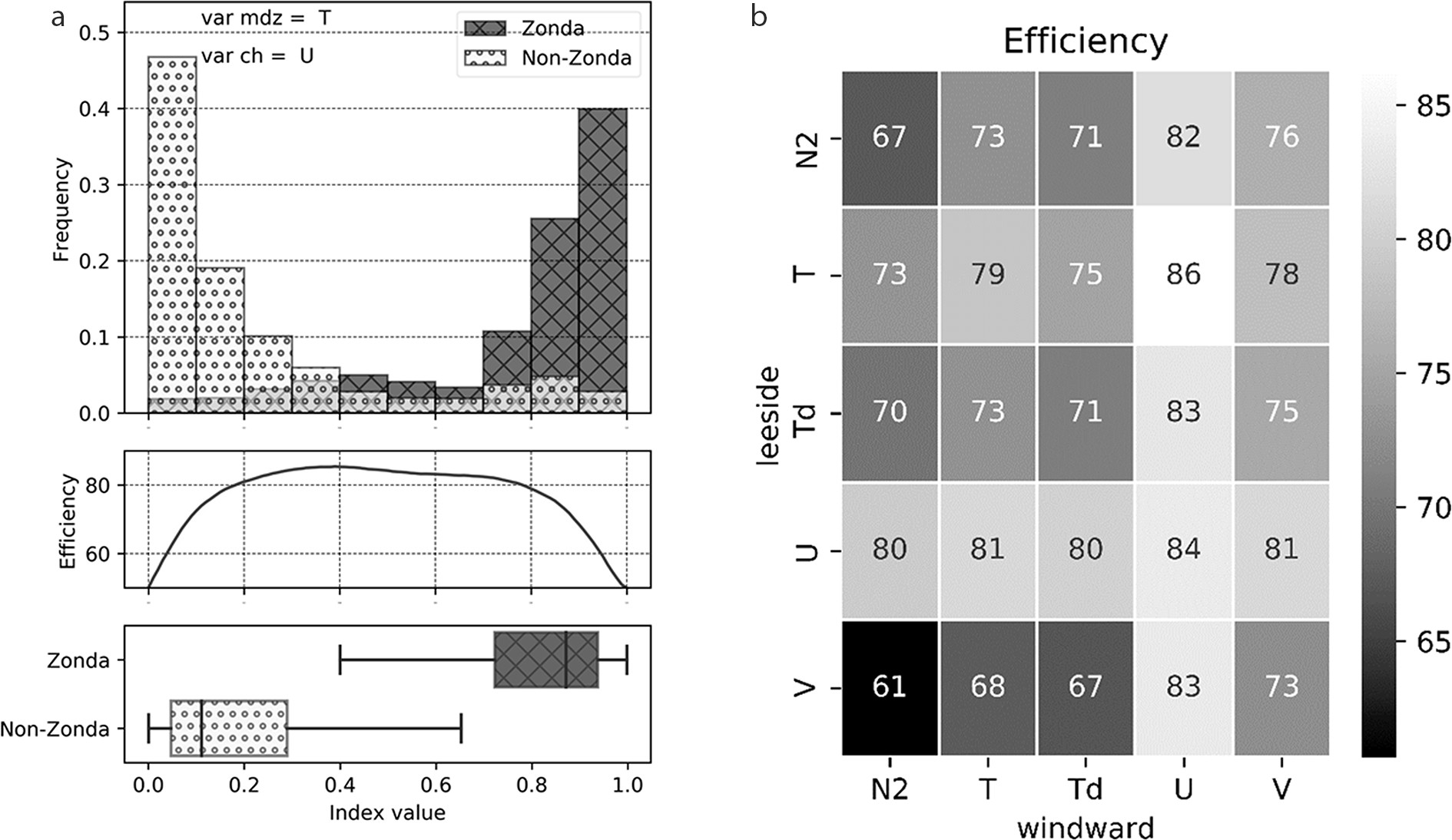
The index distribution for Zonda (dark) and for non-Zonda (light) classes, using only the vertical profile of temperature at Mendoza, the total efficiency for each cut-off value and a boxplot that indicates the dispersion of the index for the two classes are shown in Figs. 4a, 4b and 4c respectively. An index value equal to one corresponds to the Zonda class and an index value equal to zero corresponds to the non-Zonda class, whiskers represent the 3%–97% interval). If, for example, an index cut-off value of 0.5 is chosen, the number of hits for Zonda events is 80.4%, while the non-Zonda events hits represent 58.4%, and the total efficiency is below 70%. The total efficiency (Fig. 4b) reveals that, for this particular model, the best cut-off point (i.e., the value associated to the maximum efficiency) is located at 0.41, giving a total efficiency of 72.23% (86.44% hits of Zonda events and 53.84% for non-Zonda). Thus, the maximum effectiveness of the index is 72.23%, with an error of 27.77%, divided into 6.77% probability of surprise (i.e., Zonda cases that present an index value lower than the cut-off and therefore are predicted as non-Zonda) and 21% probability of false alarm (i.e., cases of non-Zonda that present an index value higher than the cut-off, so they are predicted as Zonda events). Those error values can be modified by changing the cut-off value of the index. If this value is closer to one, the non-Zonda surprises are reduced, but Zonda false alarms are augmented. Likewise, if the cut-off value is closer to zero, the Zonda false alarms are reduced and the non-Zonda surprises are augmented.
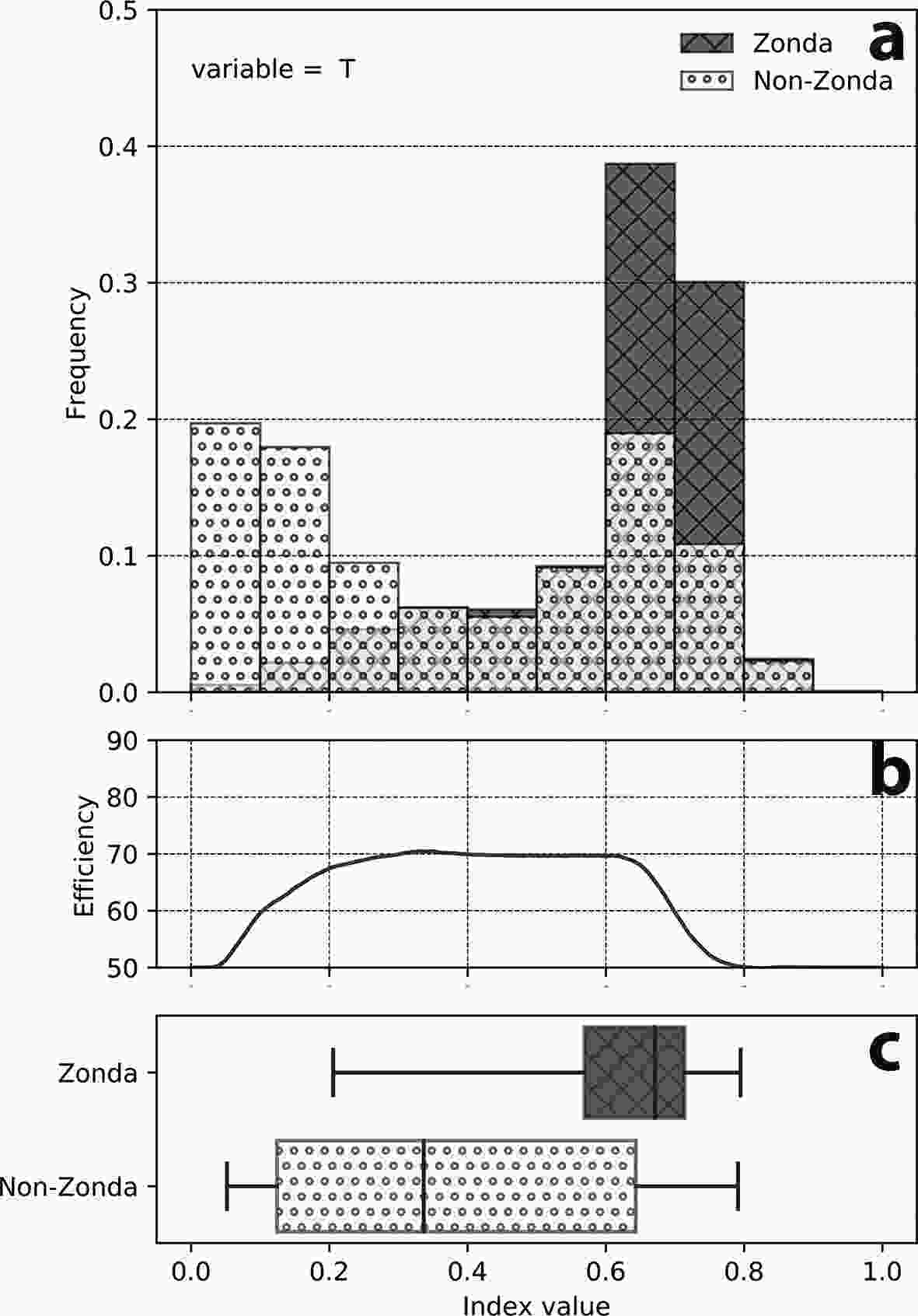
Figure 4. Leeside model for temperature. (a) Index values distribution for Zonda (dark) and for non-Zonda (light) events, (b) model efficiency according to each cut-off value, and (c) index boxplot.
For example, a cut-off value of 0.78 (50.54% efficiency) yields 1.89% and 47.56% for false alarms and surprises, respectively. Furthermore, looking at the boxplot diagrams (Fig. 4c) and their dispersion, index values higher than 0.78 correspond to the right tail of the 3rd percentile for the non-Zonda cases, while index values lower than 0.2 correspond to the left tail of the 97th percentile for Zonda cases. Therefore, for a given new sounding for which the index is calculated, values greater than 0.78 would indicate a Zonda occurrence, with an error lower than 3%. Likewise, an index value lower than 0.2 would indicate a non-Zonda occurrence with the same error. The range between those index values represents an uncertainty interval in which the index fails to discriminate between classes (at least with the previous error rates).
The same analysis is done for the windward side using the Santo Domingo vertical soundings and using both soundings at the same time (same variables). Figure 5 shows the index distribution for the zonal component of wind for the leeward (Fig. 5a), windward (Fig. 5b), and mixed (Fig. 5c) models. The windward model efficiency surpasses that for the lee side. However, the windward true positives (82.36%) are considerably lower than those obtained for the lee side (91.53%), but the true negatives and false alarms results are better. If both soundings are combined using the same variables, the model efficiency increases for some variables. The total efficiency (Fig. 5) reaches 83.57% for the zonal component of wind, slightly higher than the windward model. Again, the true positives are lower than for the leeside model, but higher than for the windward model, and false alarms are substantially reduced. Observe that the separation between classes (boxplot) is more evident in the mixed model. This indicates that moving the cut-off value of the index to the left leads to a large increase in true positives with relatively fewer surprises, but there is a higher false alarm rate and vice versa for moving the cut-off value to the right.
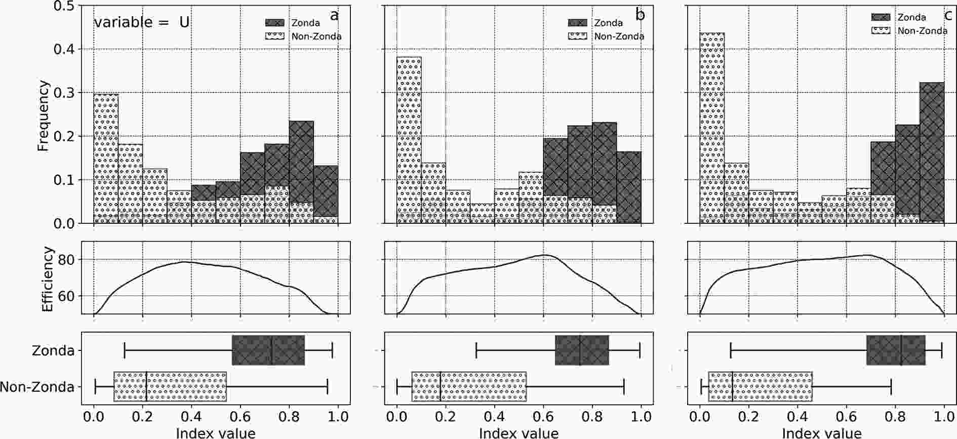
Figure 5. Same as Fig. 4 but for the zonal component model. (a) Leeside sounding, (b) windward sounding, and (c) mixed model.
If different variables for each side are combined, a new mixed model is obtained. Figure 6a shows the mixed model using temperature (T) for the lee side and U-wind for the windward side. Here, the model efficiency is maximum (86.23%), and separation between classes is greater. Note that an index value lower than 0.18 leads to 3% of Zonda surprises and a value greater than 0.9 leads to 3% of Zonda false alarms (whiskers are 3%–97%). The total efficiency for all possible combinations with one variable for each side is shown in Fig. 6b. The highest efficiency is achieved using temperature for the lee side and the U-wind for the windward side (a total efficiency of 86.31%). It is worth noting that the zonal component of the wind as a predictor is a key factor on both sides, followed by temperature on the lee side and by the meridional component on the windward side. Although this model increases the total efficiency (i.e., decreases the total error) and decreases the false alarms, the true positives and surprises results are better when only considering the leeside soundings, and the true negatives results are better for the windward soundings.

Figure 6. (a) 1-var mixed model for temperature for the lee side and zonal component of wind for the windward side and (b) the total efficiency for all possible combinations with one variable on each side.
Table 3 shows the total efficiency, the Zonda hits (true positives), the non-Zonda hits (true negatives), and the total error separated into surprises and false alarms for all variables and models. These results show that the U-wind component is the best variable predictor for all models, with a maximum efficiency of 83.57% for the mixed model. Also, the true positives are maximized for the leeward model with 91.53% and a minimum of surprises of 4.23% (leeside model, U), and true negatives and a minimum of false alarms are best predicted for the mixed model (U).
(a) Leeside Model 1-var var MDZ Total efficiency Best cut-off value True positives True negatives Error Surprises False alarms T 71.64 86.45 53.84 28.36 6.78 21.59 Td 70.56 88.95 48.12 29.44 5.53 23.91 U 79.35 91.53 64.28 20.65 4.23 16.41 V 57.11 46.12 61.4 42.89 26.94 15.95 N2 67.33 65.9 65.16 32.67 17.05 15.62 (b) Windward Model 1-var var CH Total efficiency Best cut-off value True positives True negatives Error Surprises False alarms T 65.91 49.45 77.59 34.09 25.28 8.82 Td 68.32 67.24 66.9 31.68 16.38 15.3 U 83.06 82.36 82.67 16.94 8.82 8.12 V 72.16 72 69 27.84 14 13.84 N2 58.15 68.52 41.33 41.85 15.74 26.11 (c) Mixed Model 1-var var MDZ-CH Total Efficiency Best cut-off value True Positives True Negatives Error Surprises False Alarms T 78.84 86.83 67.36 21.16 6.59 14.57 Td 70.88 83.16 54.95 29.12 8.42 20.7 U 83.57 77.97 86.57 16.43 11.02 5.41 V 72.52 72.67 69.41 27.48 13.66 13.82 N2 67.21 62.91 68.03 32.79 18.54 14.25 Table 3. Model metrics for the best cut-off index value. MDZ, Mendoza’s sounding, CH, Santo Domingo’s sounding and MDZ-CH, mixed model for same variable on each side.
-
To compare models’ skills, their metrics are shown in Table 4. Following an event-based statistic, with a POD value of 95.58% the leeward U model is the best of all. This model also has the lower MR. The POFD result is lower for the mixed model U. From an alarm-based perspective (which may be more important for a forecasting point of view), the models’ performances show that the mixed model result is better than the others, except for the MR. The False Alarm Ratio (FAR) is below 8%, and the CAR is above 92% for the mixed model U.
(a) Leeside Model 1-var Leeside var POD Best cut-off value POFD MR FAR MAR CAR T 92.73 30.00 7.27 21.07 11.18 78.93 Td 94.15 35.03 5.85 22.58 10.30 77.42 U 95.58 21.75 4.42 16.33 6.18 83.67 V 63.13 23.92 36.87 29.50 30.50 70.50 N2 79.44 21.10 20.56 20.91 20.74 79.09 (b) Windward Model 1-var Windward var POD Best cut-off value POFD MR FAR MAR CAR T 66.17 12.62 33.83 18.48 24.57 81.52 Td 80.41 19.83 19.59 19.75 19.67 80.25 U 90.33 9.49 9.67 9.52 9.64 90.48 V 83.72 18.34 16.28 17.71 16.87 82.29 N2 81.32 41.52 18.68 29.98 27.58 70.02 (c) Mixed Model 1-var Combined var POD Best cut-off value POFD MR FAR MAR CAR T 92.95 19.50 7.05 15.82 8.91 84.18 Td 90.80 29.08 9.20 21.32 13.29 78.69 U 87.62 7.20 12.38 7.93 11.29 92.07 V 84.17 18.05 15.83 17.39 16.45 82.61 N2 77.24 19.02 22.76 20.26 21.42 79.74 Table 4. Model metrics for the best-cut value. MDZ, Mendoza’s sounding, CH, Santo Domingo’s sounding, and mixed model for same variable on each side. POD (probability of detection), POFD (probability of false detection), MR (miss ratio), CAR (correct alarm ratio), FAR (false alarm ratio), and MAR (missed alarm ratio).
Figure 7 shows all metrics used for the mixed model, where the dark colors represent an enhancement of the models. The true positives are mainly controlled by the lee side (Fig. 7a). The leeside model surpasses the mixed model for T, Td, and N2. For the mixed model, the true positives are increased using U-wind, followed by temperature and dewpoint on the lee side. On the windward side, the squared Brunt–Väisälä frequency, aside from U, also increases the true positives. To the contrary, the true negatives (Fig. 7d) appear to be controlled by the windward side, in a similar case as the true positives. According to the definition of the metrics, the surprises (Fig. 7g), POD (Fig. 7e), and MR (Fig. 7c) result in similar patterns to those of the true positives and, false alarms (Fig. 7b), and FAR (Fig. 7f), and POFD (Fig. 7h) results in similar patterns to the true negatives. The MAR (Fig. 7i) is a combination of both patterns.
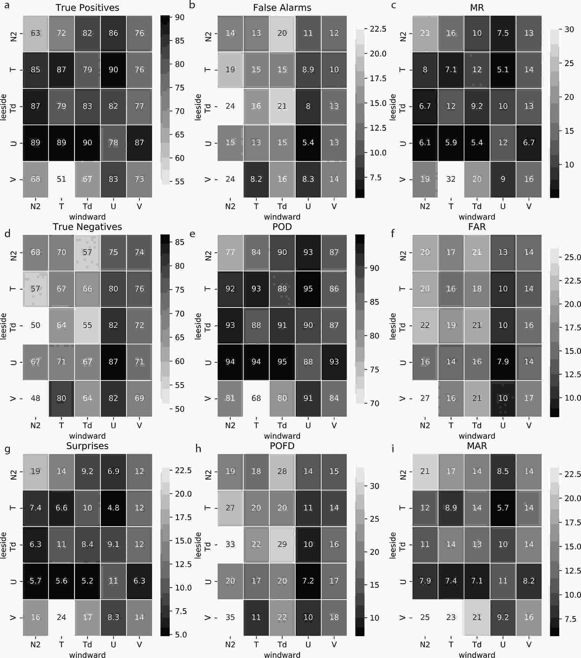
Figure 7. 1-var mixed model metrics: true positives (a) and negatives (d), surprises (g) and false alarms (b), POD (e), POFD (h), MR (c), FAR (f), and MAR (i).
So, it is clear that the leeside soundings are better predictors for the detection of Zonda events, while the windward side helps to improve false detections and alarms.
-
The discriminant sounding (
$\boldsymbol{A}$ vector, see section 2.2.3) between Zonda and non-Zonda classes obtained from the PCA is shown in Fig. 8. For the lee side (Fig. 8a), this vertical sounding is characterized by positive temperature anomalies between 850 hPa and 600 hPa and negative anomalies in upper levels. The low-level temperature increase is accompanied by positive anomalies of dewpoint near the surface and negative anomalies between 800 hPa and 500 hPa. The zonal component of wind shows negative anomalies at low levels with two relative maximums of positive anomalies at 700 hPa and 400 hPa, while the meridional component is the opposite of the previous one (not shown). The squared Brunt–Väisälä frequency has positive anomalies at low and upper levels with negative anomalies at midlevels.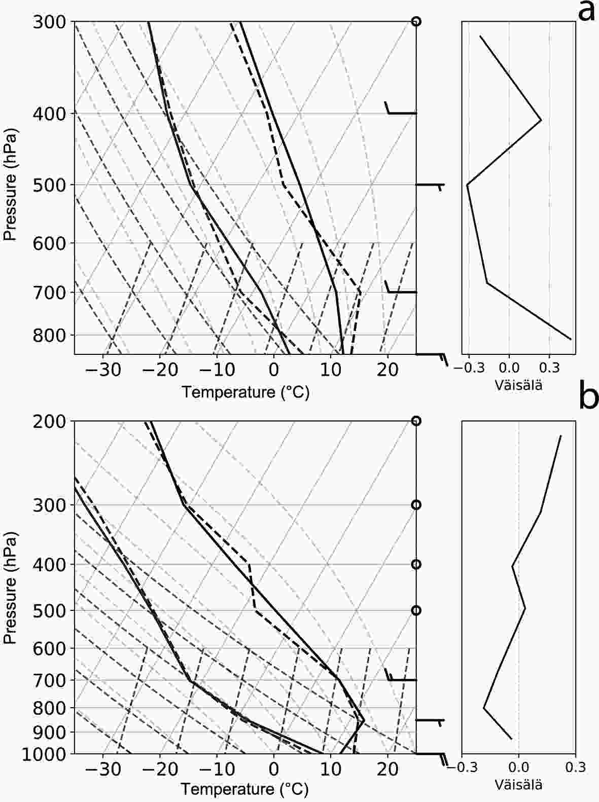
Figure 8. (a) Discriminant sounding between Zonda and non-Zonda classes for the 1-var models for the lee side and (b) for the windward side. Since the discriminant soundings are anomalies with respect to the mean profile, temperature and dewpoint temperature variables are multiplied by a factor of five and added to the mean sounding to better appreciate the differences with the mean sounding. The zonal component (U) of the wind is multiplied by a factor of 10 as anomalous values (i.e., the mean sounding is not added). The meridional component is omitted due to its lesser relevance in the models. The squared Brunt–Väisälä frequency presents the original values of the discriminant sounding.
This leeside discriminant sounding represents a sounding that tends to become unstable at midlevels due to strong heating at low levels and cooling at midlevels, with greater drying at 700 hPa and moistening near the surface. Above this layer, the sounding tends to normalize in humidity and temperature, approaching the climatological one, but with positive anomalies of zonal wind and more static stability at 400 hPa. According to this profile, a stable layer near the surface is present and the windstorm probably is already present at 700 hPa (the soundings are previous to the event at land level) with a NW component of wind. Also, the upper-level jet streak could be present at this time.
For the windward model (Fig. 8b), the vertical sounding is characterized by a temperature positive anomaly near the mountain top, between 500 hPa and 400 hPa, with a stable region above this layer. The layer below this region has negative anomalies of the squared Brunt–Väisälä frequency, with U-wind anomaly maximums at 700 hPa and near the surface with opposite values. The meridional component acts only at low levels (not shown).
So, in accordance with the highest efficiency values to discriminate between classes, a vertical sounding that presents positive U-wind (westerly) anomalies at 700 hPa on the windward side and two maximums of positive anomalies on the lee side are the key predictors for Zonda occurrence. The leeside U-wind anomalies correspond to the presence of Zonda at midlevels and to the jet streak in upper levels. This vertical structure could be accompanied by a temperature inversion (and a stable layer above) near the mountain top windward side and significant drying at midlevels on the lee side.
-
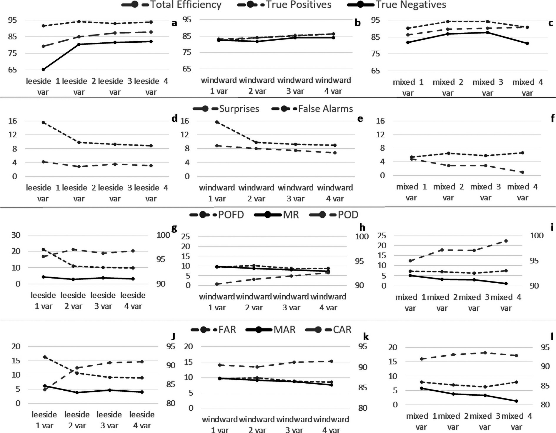
If more variables are added to the model, an efficiency gain is observed, especially for the lee side. Figure 9 (a, d, g and j) shows the best result (i.e., best variables combinations) of the metrics for the leeside models by adding more variables. The total efficiency and the true negatives present a considerable increase from one variable to two, with little variation when adding more than two. The efficiency goes from 80% to 88%, and the true negatives go from 65% to 82%. The true positives seem not to change much by adding more variables and present a maximum for two variables. False alarms are also reduced, but surprises are not. The event-based statistic presents a considerable diminution in the POFD and a rise in the POD between one and two variables, but the MR remains almost constant. From an alarm-based perspective, the CAR and the FAR are improved, and the missing alarm ratio does not present any changes.
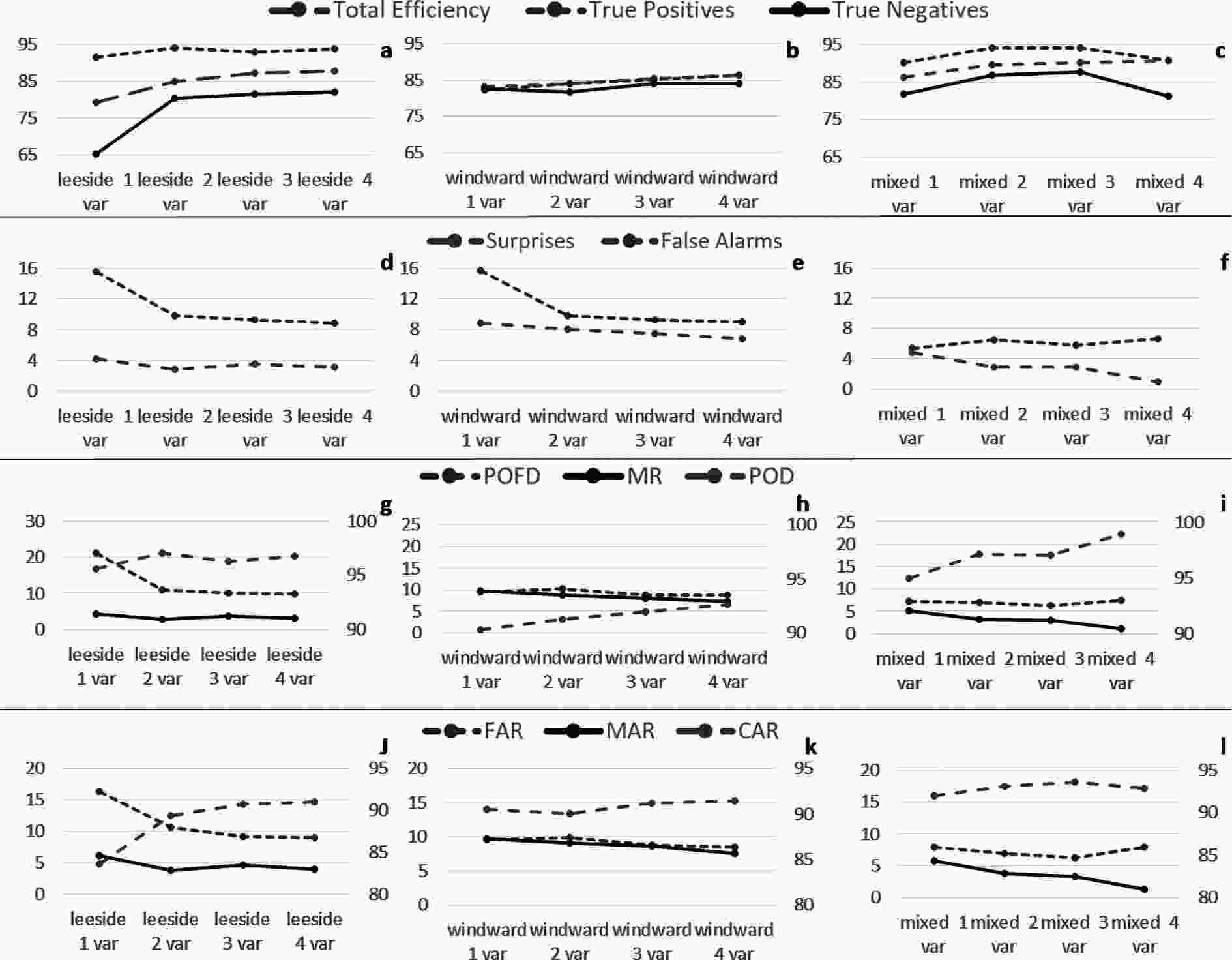
Figure 9. Total efficiency, true positives and true negatives, false alarms, POD (right axis), POFD, MR, CAR (right axis), FAR, and MAR for the lee side (a, d, g, and j), for the windward side (b, e, h, and k), and for mixed models (c, f, i, and l).
For the windward side (Figs. 9b, e, h and k), the total efficiency and true negatives increase almost linearly by adding more variables, while true negatives sightly increase adding more variables. Surprises decrease 2 point up to four variables, and the false alarms highly improve going from one to two variables. The event-based statistic presents almost no change in the POFD (or even decrease), the POD linearly rises, and the Missing Ratio presents a diminution. From an alarm-based perspective, the False Alarm Ratio and the Missing Alarm Ratio decrease, improving the model. The Correct Alarm Ratio increases 1.5 times going from two to four variables.
The mixed model (Figs. 9c, f, i, and l) presents its maximums of true negatives and positives for two and three variables, while the total efficiency reaches its maximum for four variables but almost with a small change for two, three, and four variables. In this model, the false alarms seem not to improve by adding variables, as observed for the previous models. From an event-based perspective, the POD increases 4 point (from 94.94% to 98.9%) from one to four variables and the MR also presents an improvement, but the POFD does not. Finally, the MAR is highly reduced, while the CAR and FAR reach their optimal values for three variables.
It is clear that the mixed models turn out to be significantly better than the separate models. On the other hand, adding a greater number of variables to the mixed model does not always improve the metrics, as is the case of the true positives and negatives, POFD, CAR, and FAR, whose maximums are reached with two or three variables and not with four (Table 5).
Mixed Efficiency True Positives True Negatives Surprises False Alarms POD POFD MR FAR MAR CAR 1-var 86.31 90.36 81.83 4.82 5.41 94.94 7.20 5.06 7.93 5.71 92.07 2-var 89.66 94.34 86.97 2.83 6.52 97.09 6.97 3.34 6.91 3.74 93.09 3-var 90.41 94.16 87.66 2.91 5.81 97.00 6.17 3.00 6.36 3.36 93.64 4-var 90.77 90.88 81.38 0.86 6.56 98.90 7.47 1.05 7.92 1.36 92.94 Table 5. Mixed model metrics for the best combination.
Figure 10 shows the best mixed models (considering the total efficiency) for two, three, and four variables. As can be noted, the separation between classes is more evident (than the 1-var mixed model), causing the uncertainty interval to decrease considerably. The Zonda 25th–75th percentile intervals are reduced to the index interval [0.8–1] (the 1-var mixed model is [0.7–0.9]), while for non-Zonda cases, this interval is reduced to [0–0.2] (the 1-var mixed model is [0.0.5–0.45]). This value is greater than the 3rd percentile of the Zonda cases. For the 2-var mixed model (Fig. 10a), an index value lower than 0.19 leads to only 3% surprises for Zonda events. Unlike the 1-var mixed model, the 25th percentile, which was located at 0.7, is above 0.78, and the 75th percentile moves towards a value of 0.98 in the 4-var mixed model (Fig. 10c). In this way, surprises are considerably reduced. The total efficiencies for all two-variable mixed models (figure not shown) clearly show maximums by considering T-U (89.66%) and T-N2 (89.2%) for the lee side combined with T-U for the windward side.

Figure 10. Best mixed models considering the total efficiency for two, three, and four variables. (a) 2-var mixed model for temperature and zonal component for each side. (b) 3-var mixed model for temperature, zonal component, and squared Brunt–Väisälä for both sides. (c) 4-var mixed model for temperature, zonal and meridional components, and squared Brunt–Väisälä for the lee side and temperature, dewpoint, zonal component, and squared Brunt–Väisälä for the windward side.
Table 6 shows the best combinations of variables for the leeside, windward, and mixed models with two, three, and four variables. It can be seen that the variables U, N2, and T and Td (to a lesser extent) are the best classifiers between Zonda and non-Zonda soundings. In addition, note the little difference that exists by adding a greater number of variables. For example, for the mixed model, there is a difference of 1.02 and 1.11 points between the 2-var model and 3-var and 4-var models, respectively. These differences are greater when considering the leeward model, where the differences in efficiency between two and three variables is almost 2.5%, and between three and four variables the difference is 0.5%. The windward models do not seem to be very sensitive to the addition of variables.
(a) Leeside Model 2-var Efficiency windward model 2-var Efficiency mixed model 2-var Efficiency U-N2 84.83 U-V 84.12 T-U−T-U 89.66 T-U 83.28 U-N2 83.21 T-N2−T-U 89.21 U-V 79.83 Td-U 83.08 T-N2−U-V 89.07 Td-U 79.44 T-U 82.78 T-U−U-V 88.84 T-Td 77.11 T-V 75.35 T-U−U-N2 88.84 T-N2 73.75 V-N2 75.06 T-U−Td-U 88.68 T-V 72.46 Td-V 73.78 T-Td−U-V 88.41 Td-N2 71.08 T-Td 70.93 T-V−T-U 88.33 Td-V 70.78 T-N2 68.59 T-Td−T-U 88.27 V2-N2 69.18 Td-N2 68.53 T-N2−U-N2 88.25 (b) Leeside Model 3-var Efficiency windward model 3-var Efficiency mixed model 3-var Efficiency T-U-N2 87.26 U-V-N2 85.34 T-U-N2−T-U-N2 90.68 Td-U-N2 84.38 Td-U-N2 84.97 T-Td-U−T-U-N2 90.41 T-U-V 83.87 T-U-V 83.71 T-Td-U−T- Td -U 90.03 U-V-N2 83.81 Td-U-V 83.66 T- Td -U−T-U-V 89.94 T-Td-U 83.47 T-U-N2 83.28 T-V-N2−T-U-N2 89.86 Td-U-V 80.72 T-Td-U 83.25 T-U-N2−T- Td -U 89.78 T-Td-N2 78.10 T-V-N2 77.51 T-U-V−T-U-N2 89.63 T-Td-V 78.01 T-Td-V 76.62 T-U-N2− Td -U-N2 89.39 T-V-N2 74.25 Td-V-N2 74.85 T- Td -V−T-U-N2 89.22 Td-V-N2 72.75 T-Td-N2 74.43 T-U-N2−U-V-N2 89.13 (c) Leeside Model 4-var Efficiency windward model 4-var Efficiency mixed model 4-var Efficiency T-Td-U-N2 87.75 Td-U-V-N2 86.34 T-U-V-N2−T-Td-U-N2 90.77 T-U-V-N2 87.25 T-U-V-N2 85.65 T-Td-U-V−T-Td-U-N2 90.26 Td -U-V-N2 85.48 T-Td-U-N2 85.60 T-Td-U-N2−T-Td-U-N2 90.22 T-Td-U-V 84.64 T-Td-U-V 84.86 T-Td-U-N2−T-U-V-N2 89.99 T-Td-V-N2 79.01 T-Td-V-N2 79.47 T-Td-V-N2−T-U-V-N2 89.83 Table 6. Best 10 mixed models considering the total efficiency for two and three variables and best 5 mixed models for four variables. First column: leeside 2-, 3- and 4-var best 10 models, with second column for the windward side and third column for the mixed models.
From Table 6, it is also concluded that, regardless of whether there is a single sounding or soundings for both (windward and leeward) for the forecasting day, the efficiency values of the models presented here can be high, with a difference of less than 5% (this is the case between the windward and mixed models). However, the presence of the leeside sounding is of greater importance in obtaining greater precision in the detection of Zonda events and in reducing false alarms.
-
The combination of soundings on both sides of the Andes produces a slight change in the obtained profiles due to the change in the fit coefficients of the new model. The discriminant sounding between Zonda and non-Zonda classes obtained from the PCA is shown in Fig. 11 for the 4-var mixed model.
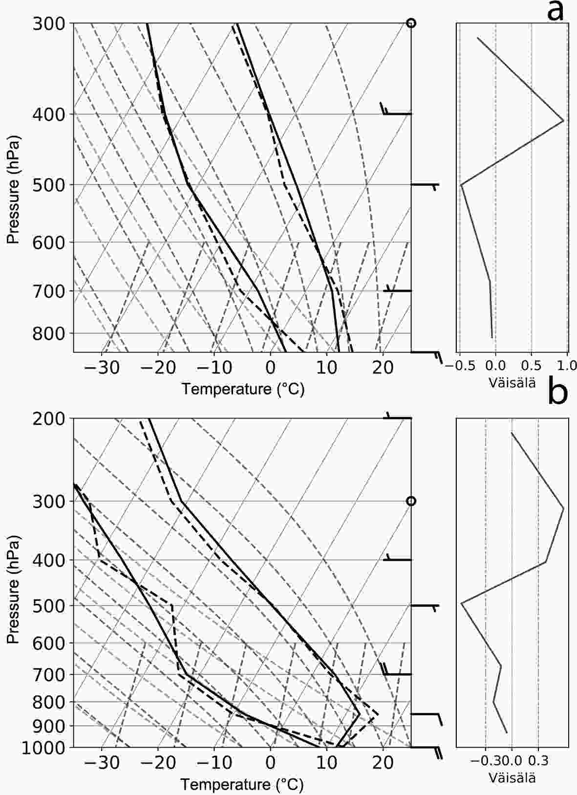
Figure 11. Discriminant sounding between Zonda and non-Zonda classes for the 4-var model (a) for the lee side and (b) for windward side.
This model presents a leeside (Fig. 11a) vertical structure characterized by positive temperature anomalies between 850 hPa and 650 hPa and a minimum of negative anomalies at midlevels, which tends to represent an unstable profile. The vertical structure of dewpoint presents negative anomalies at 700 hPa and a maximum of positive anomalies near the surface. The vertical structure of U anomalies correlates well with the presence of vertically (backward) propagating waves, with an alternating pattern of negative and positive anomalies, with a maximum of negative anomalies at 850 hPa and positive anomalies at 400 hPa. The vertical sounding is accompanied by a stable layer at 400 hPa and a statically more unstable layer at midlevels.
The windward (Fig. 11b) discriminant sounding presents positive anomalies at 850 hPa and negative anomalies in upper levels. Similarly to the lee side, this sounding becomes unstable. This vertical sounding does not present a temperature inversion like the 1-var model (Fig. 8b). Positive anomalies of dewpoint can be seen near the surface and at 500 hPa, while the negative anomalies are observed at 800 hPa and at 400 hPa. The U-wind anomalies present strong maximums at 700 hPa and near the surface, with opposite values. Like for the lee side, positive and negative changes in the zonal component anomalies can be seen and the vertical sounding is accompanied by a stable layer above 450 hPa and a statically more unstable layer at 500 hPa.
-
This paper represents an improvement over work previously carried out. In Otero et al. (2018), soundings were used for T and Td along with surface values for the same variables only for the lee side. The development of the Zonda phenomenon is closely related to the vertical structure of the atmosphere, where the mountain height, the buoyancy frequency, and incident wind control the mountain wave activity and the dynamics of downslope wind, which the previous work did not consider. Here, the characteristics on both sides of the barrier of stability, wind, temperature, and humidity that are more favorable for this type of event could be known. Thus, in this new paper, progress in understanding the characteristics of the atmosphere, both windward and leeward, prior to the development of a Zonda event, is made. The efficiency values obtained in this new work are even higher, without the need of surface data. Statistical values (event-based and alarm-based model metrics) associated with the model were also recognized and can provide additional information for decision makers.
The results show that this index model is able to discriminate between Zonda and non-Zonda events with an effectiveness close to 80% using only one variable on one side of the barrier, increasing to almost 84% by using one variable on each side of the barrier. These values of effectiveness in class separation increase to almost 91% using four variables on each side of the Andes. The number of Zonda hits is mainly captured by the leeside soundings, while the non-Zonda hits are mostly controlled by the windward soundings. The soundings combination in the mixed model produces better class separation and significantly reduces false alarms. The correlation values between the real index and the estimated index increase considerably when adding variables, reaching values of more than 0.84.
It is found that the zonal component of the wind (U-wind) on both sides and the windward temperature are the key variables in class discrimination. The true positives and surprises are mainly controlled by the leeside sounding, while the POFD improves with the mixed model (i.e., by adding the windward sounding). Even though mixed model maximum efficiency, surprises, POD, MR, and MAR turn out to be with four variables on each side, the true positives and negatives, POFD, CAR, and FAR reach their maximums with two or three variables.
The vertical profile that best succeeds to discriminate between Zonda and non-Zonda is characterized by a leeside sounding that tends to become unstable at midlevels and presents two wind maxima, possibly associated with the foehn effect at low levels and the presence of the jet streak at high levels. On the windward side, there is also a wind maximum at 700 hPa, accompanied by a relatively more stable layer near the top of the barrier.
The methodology used in this work could be replicated in any region that has sounding data (preferable on both sides of the barrier). Although the results obtained may vary from region to region, it could represent a valuable tool for this type of phenomena that are so difficult to forecast. After determining the discriminant vector A from the PCA and the multiple regression model, the probability index for Zonda/non-Zonda occurrence can be easily obtained to forecast the Zonda occurrence up to 24 hours in advance.
This work ensures, in a preliminary way, that the PCA is a useful tool in the detection of the Zonda phenomenon. However, using more data (such as surface values or reanalysis) could significantly improve the efficiency of the model. In addition, the monthly anomalous soundings were tested, but the model did not significantly improve, so it was decided not to consider separate seasons. The seasonality could affect the frequency of events but not the atmospheric conditions (synoptic and local) under which they originate.
| Predicted | ||
| Yes (Zonda) | No (non-Zonda) | |
| Observed (Zonda) | TP | FN |
| (Hit Zonda) | (surprise) | |
| No event (non-Zonda) | FP | TN |
| (Zonda False Alarm) | (Hit non-Zonda) | |


 AAS Website
 AAS WeChat