Determination of Surface Precipitation Type Based on the Data Fusion Approach

According to the Glossary of Meteorology, the term “precipitation” denotes “all liquid or solid phase aqueous particles that originate in the atmosphere and fall to the earth’s surface” (American Meteorological Society, 2019). In practice, the atmospheric precipitation type (PT) can take liquid, solid or mixed forms. Liquid precipitation refers to drizzle and rain, while mixed precipitation includes freezing drizzle, freezing rain, and a mix of rain and snow. Solid precipitation consists of snow, snow grains, ice pellets, hail, snow pellets/graupel and ice crystals (Thériault et al., 2010; Reeves et al., 2014).

PTs are strongly determined by thermodynamic and boundary-layer processes. The vertical temperature profile, horizontal and vertical air motion, moisture content, cloud microphysics, size distribution of droplets, precipitation rate, hydrometeor interactions, and their initial-phase composition all have a strong influence on the resulting surface PT (Reeves et al., 2016).

In operational forecasting, the temperature profile plays typically the most important role in the determination of PT (Reeves et al., 2014; Stewart et al., 2015). In midlatitudes, the classic example of a rapid transitions between solid, liquid or mixed PT is a passage of a warm front composed of a warmer air layer (T > 0°C) overlaying a colder one (T < 0°C) (Groisman et al., 2016; Matte et al., 2019). Hydrometeors, which are in a solid state in the early stages, begin to melt as they fall through the warmer air layers. The degree of melting depends on the ambient temperature and size of condensation nuclei. Moreover, the collision of ice pellets and snowflakes can also impact the degree of melting (Thériault et al., 2010; Kämäräinen et al., 2017).

Typically, two main procedures have been used to determine PT in atmospheric models (Matte et al., 2019). The first uses microphysics equations to predict the mixing ratio and concentration of hydrometeors (Morrison and Milbrandt, 2015) while the second, the so-called “diagnostic approach”, is more frequently applied. The latter is based on the vertical profile of variables such as air temperature, relative humidity, mixing ratio and/or lapse rate applied as proxies for determination of PT (Bourgouin, 2000; Reeves et al., 2014; Czernecki et al., 2019).

Proper identification of PT is important for the initial stage of numerical modeling. The initial error may increase uncertainty in the forecasting of PT, which may appear later as a systematic error. A proper identification of rain and snow is less troublesome than mixed PT. The latter is usually defined as a mixture of partially melted larger hydrometeors and/or completely melted smaller ones (Kain et al., 2000). The degree of partial melting has quite an influence on the PT. An additional problem is that microphysical schemes in operational numerical weather prediction (NWP) models often do not account for mixed-phase hydrometeors (Thériault and Stewart, 2010). Another reason for the uncertainty in forecasting the specific PT is related to the reliability of NWP models. In some situations, a variation of only 0.5°C is sufficient to induce a transition between different phases of hydrometeors, while the forecast uncertainty is usually larger (0.5°C–4.0°C; Bourgouin, 2000; Coniglio et al., 2010; Reeves et al., 2014).

Given these limitations, it is not surprising that operational forecasting of PT is often based on both the explicit and the implicit methods. The lower-tropospheric mixing ratio and air temperature are used as input data to determine the PT by explicit methods, while the temperature and moisture of the ambient environment are used by implicit methods. However, usually none of the two aforementioned methods is significantly better (Reeves et al., 2014).

The PT and the possibility of its prediction are crucial for decision making in terms of economics and human health protection, especially with respect to significant climate change in the foreseeable future. According to IPCC (2013), the increase in global mean air temperature will be accompanied by an increasing number of hazardous weather conditions like heavy precipitation, large hail, freezing rain and icing. This will also have a major financial impact, especially in midlatitudes (e.g. Vajda et al., 2014; Borsky and Unterberger, 2019). The currently observed climate change also impacts the ratio of specific PTs, with a systematic increase in the probability of liquid precipitation, and a general shift toward more rain and less snow (Mekis and Vincent, 2011), as well as an increase in freezing rain (Hanesiak and Wang, 2005). According to Cheng et al. (2011) and Lambert and Hansen (2011), future occurrence of freezing rain over North America will be shifted substantially northward.

Accurate forecasting of the PT is important in numerous areas of human life, but especially in the field broadly defined as social safety (Ikeda et al., 2013). Therefore, we want to answer the question: “How can machine learning techniques applied in observational and NWP data help to improve the recognition of the surface PT?” We aim to achieve this goal by estimating the accuracy of the post processing–based solution that might be applied by means of machine learning (ML) algorithms with a combination of multiple data sources, leading to further improvements in NWP-based forecasting systems. Among many modeling attempts that have been made for identification of PTs (Allen et al., 2015; Gagne et al., 2017; Ukkonen et al., 2017), only a few used a combination of NWP data with real-time remote sensing observations (Gagne et al., 2017; Czernecki et al., 2019). Therefore, it is especially valuable to investigate the application of the so-called data fusion approach, which is becoming increasingly popular thanks to advances in computational power capacity (Gagne et al., 2017; McGovern et al., 2017; Czernecki et al., 2019). In this paper, three PTs (according to SYNOP report codes) were taken into consideration: (i) liquid precipitation (drizzle and rain); (ii) mixed precipitation (freezing drizzle, freezing rain, mix of rain and snow); and (iii) solid precipitation (snow, snow grains, ice pellets, sleet, snow pellets/graupel, ice crystals).

Three data sources are used to evaluate PT: surface synoptic observations (SYNOP reports), meteorological radar data (maximum column reflectivity), and ERA5 reanalysis on model levels (full names of parameters and their abbreviations are presented in Table 1). Data concern the area of Poland and the period from 2015 to 2017. All observations are merged into one homogeneous database by assigning radar reflectivity and reanalysis-derived variables to the corresponding geographical location of observed PT. In the following subsections, further details on each dataset are provided.

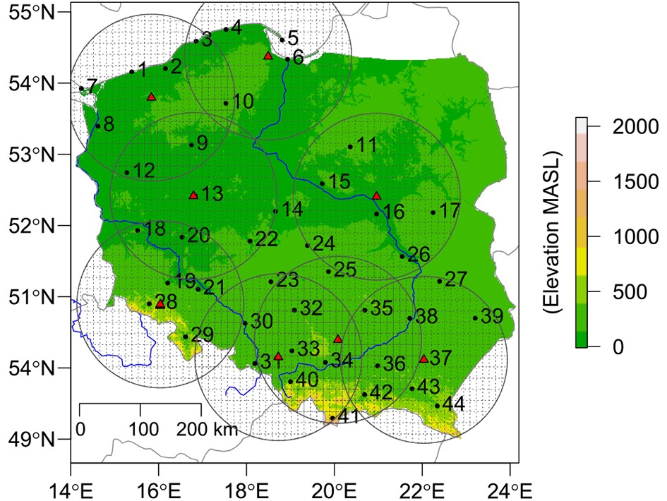
Surface synoptic observations with hourly resolution were taken from the 44 meteorological stations maintained by the Polish Institute of Meteorology and Water Management−National Research Institute (IMGW-PIB; Fig. 1). A total of 8645 manned observations of PT were considered. PTs were gathered into three main categories according to the subdivision used in the METAR reports for: (1) liquid precipitation (drizzle and rain); (2) mixed precipitation (freezing drizzle, freezing rain, mix of rain and snow); and (3) solid precipitation (snow, snow grains, ice pellets, sleet, snow pellets/graupel or ice crystals) (Thériault et al., 2010; Reeves et al., 2014). The sample size was 6269 (72.4%), 98 (1.1%), and 2278 (26.5%) cases (percentages) for the aforementioned categories, respectively. Hail events were not taken into account as we found only 12 hail reports in the period of analysis and most precipitation algorithms consider them usually as a separate category (Czernecki et al., 2019). Additionally, information about other near-surface meteorological variables such as air temperature, specific humidity and wind speed were also taken into account.

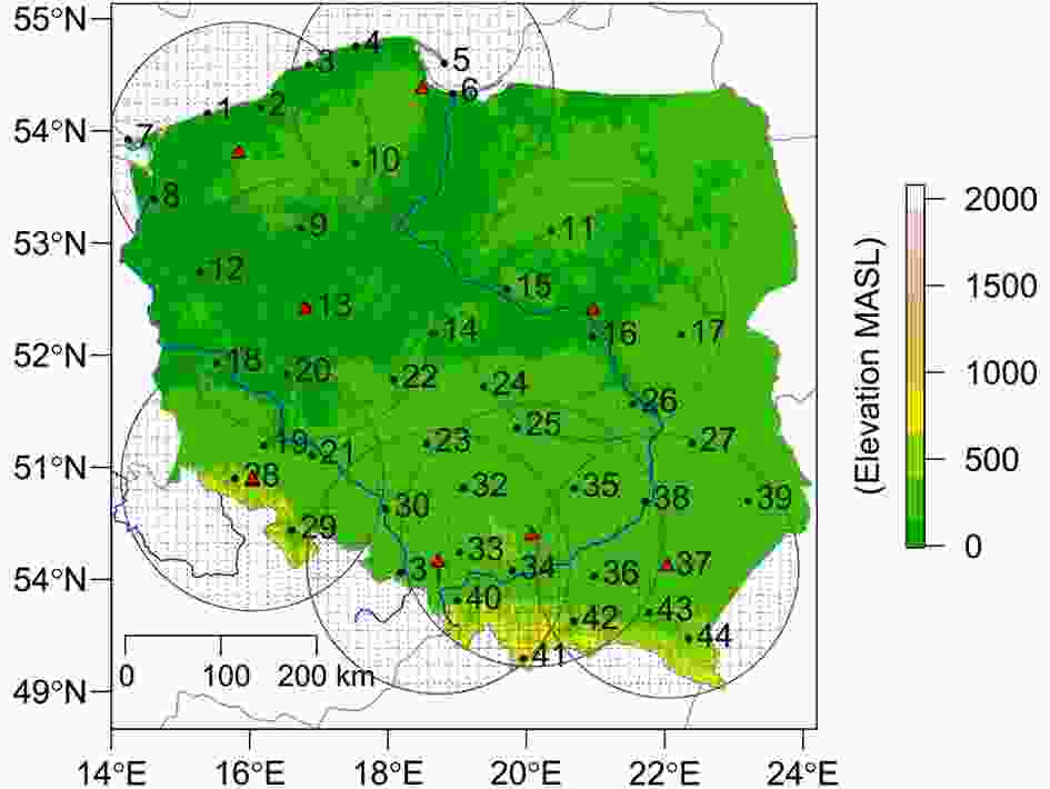
Figure 1.  Location of meteorological radar sensors (red triangles) with 125-km buffer zones. Black points and numbers show the locations of meteorological stations. Black dashed lines indicate ERA5 grid nodes.

Reanalysis allows generation of a synthetic dataset in a location with no observational record or for a longer period of time regardless of possible inhomogeneities in in-situ measurement (e.g., relocation of stations, data gaps, changes in measuring techniques) (Allen and Karoly, 2014; de Leeuw et al., 2015; Ukkonen et al., 2017).

In this study we used ERA5, whose production started in 2016 (Hersbach et al., 2020). The ERA5 reanalysis is distributed with a 0.25° horizontal grid spacing, 137 vertical sigma levels, and a 1-h temporal resolution. The nearest observational dataset from a meteorological station was assigned to a nearest grid point (by geographical distance) from ERA5 that corresponds to a given location and time (Fig. 1). For the purposes of this analysis, air temperature, specific humidity, and zonal and meridional winds were interpolated to vertical profiles (from ERA5 hybrid-sigma model levels) for altitudes of 2 (10 for wind components only), 100, 250, 500, 1000, 1500, 2000, 2500 and 3000 m above ground level (AGL). In addition, the height of the freezing level and vertical temperature lapse rate in the 0–3000 AGL layer were also computed to account for melting and mixing processes. The depth of the melting layer was another variable that was also computed, and defined as a layer within 0–1 km AGL where air temperature was above 0°C. This parameter was calculated based on vertically (linearly) interpolated data with a resolution of 1 m. In total, 29 parameters derived from ERA5 reanalysis were taken into account (Table 1).

The POLRAD weather radar network, maintained by IMGW-PIB, consists of eight C-band Doppler radars: Meteor 500C (Poznań, Brzuchania, Świdwin), Meteor 1500C (Legionowo, Gdańsk), and the dual-polarimetric Meteor 1600C (Pastewnik, Rzeszów, Ramża) of Selex ES (formerly Gematronik) (Ośródka et al., 2014) (Fig. 1). In this study, we used a product of maximum radar reflectivity (CMAX). The original temporal resolution of 10 min was aggregated to a maximum hourly value and then regridded from a 1 km to 0.25° grid to match the ERA5 resolution. For each SYNOP report, the nearest (by geographical distance) grid point (and corresponding timeframe) from POLRAD was assigned. In order to account for the decreasing magnitude of the radar beam along with an increasing distance, our results consider only those stations located no more than 125 km away from the radar site.

ML algorithms enable the analysis of large amounts of data and can deliver more accurate results than traditionally applied statistical linear regression models. Classification problems (as stated in this study) can be solved by a supervised learning approach that learns on the basis of the input data and then uses an uncovered regularity from historical data to classify new observations. That classification problem may be defined as a binary (e.g., precipitation is liquid or not?) or multi-class form (as in this case: liquid, solid or mixed precipitation). The Random Forest (RF) results were classified as the probability that allows to distinguish between mixed, liquid, and solid PTs. The RF implementation was performed in the R programming language within the “ranger” package (Wright and Ziegler, 2017). The model was built with 100 trees and split into a minimum of 5 nodes for each variable. Model parameters not mentioned in the above part were set as default based on the “ranger” and “caret” packages of the R programming language (Kursa and Rudnicki, 2010; R Core Team, 2015; Kuhn, 2020).

To avoid model overfitting, a bootstrap resampling was used. This was done by splitting the training dataset into 10 folds, with 30% of the original data removed from each fold. Also checked was that no more than 60% of mixed precipitation records could be used in each of the cross-validation chunks, to avoid overfitting for the smallest class. The model was built on a clipped dataset of a near-surface air temperature ranging from −4.0°C to 5.6°C. This was done in order to avoid classification of trivial cases where only one type of surface PT occurred, and could potentially bias model performance. The trimmed database for modeling purposes consisted of 2261 cases with 1091 (48.2%) of liquid, 98 (4.3%) mixed and 1077 (47.5%) solid PT events.

It is worth mentioning that most of the meteorological parameters considered are cross-correlated. Therefore, the decision to apply the RF algorithm was related to its robustness with respect to multicollinearity issues (in terms of obtained accuracy). In particular, it is relevant for a mixed type of precipitation where a significant portion of the signal might overlap with other PTs. Prior studies have indicated that, in such situations, RF will outperform other ML methods (Gagne et al., 2017; McGovern et al., 2017; Czernecki et al., 2019), considering also rare and severe weather events.

Although the overall accuracy of ML models is one of the main reasons for choosing a decision-tree model, it is also important to underline other advantages of RF algorithms. These are related to finding relevant features that impact the modeled process, as well as reducing the number of predictors used. To perform the abovementioned steps, the “Boruta” algorithm was used (Kursa and Rudnicki, 2010). The calculated “relative influence” (Friedman, 2001) confirmed that all 30 chosen variables (Table 1) are relevant and contain a signal stronger than random noise. This means that all parameters are potentially useful in determining surface PTs. The variable importance was computed separately for each type of precipitation (liquid, solid, mixed) as well as for multi-class combinations. Scaled values (i.e., max = 100) of the variable importance indicate which predictors contribute the most to the developed model, making it also possible to specify the top 15 parameters that impact a given surface PT.

In order to address the question as to whether the proposed RF model shows any added value, it was decided that a baseline model be created using simplified classification trees. It is quite common forecasting practice to use T2 and T1000 values to determine the PT based on historical data or user experience. A similar solution was adopted in this study with a tree being built for a single variable that splits the main node into two sub-groups. This process is then applied in each sub-group, but in order to avoid very deep trees it was decided that a maximum of three nodes would be used. These models were built on the same database as for the RF model, but without application of the cross-validation procedure and for the single-class approach (i.e., single PT vs. others).

The obtained threshold values for the three models remain in agreement with results described later on and presented in Figs. 2 and 3. For solid PT, the classification tree is based on threshold values of T2 = 0.85°C and T1000 = −1.68°C; for mixed, T2 = 0.36°C, T2 = 1.45°C and T1000 = −1.02°C; and for liquid PT the classification tree uses T2 = 0.85°C and T1000 = −0.97°C.

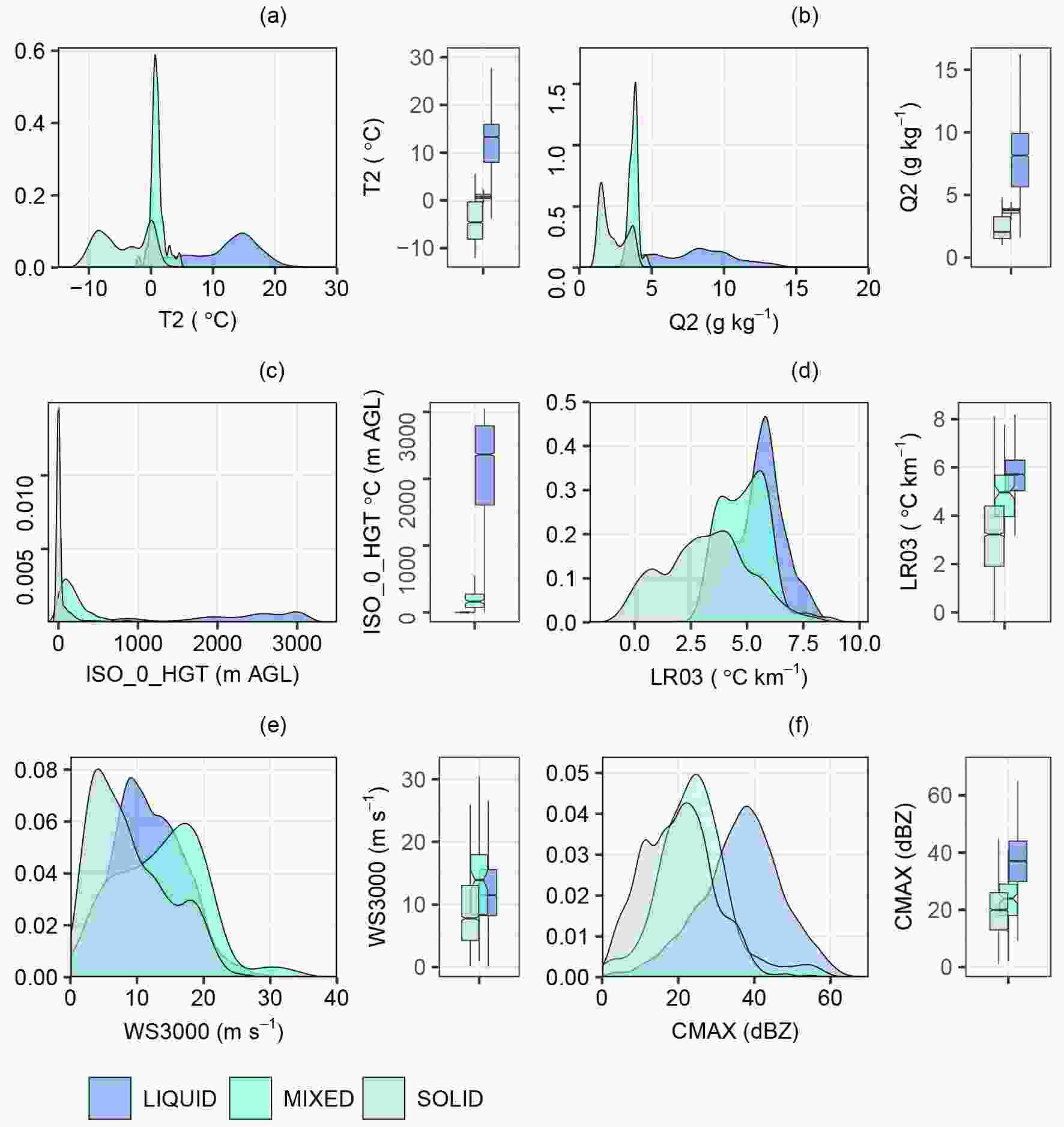
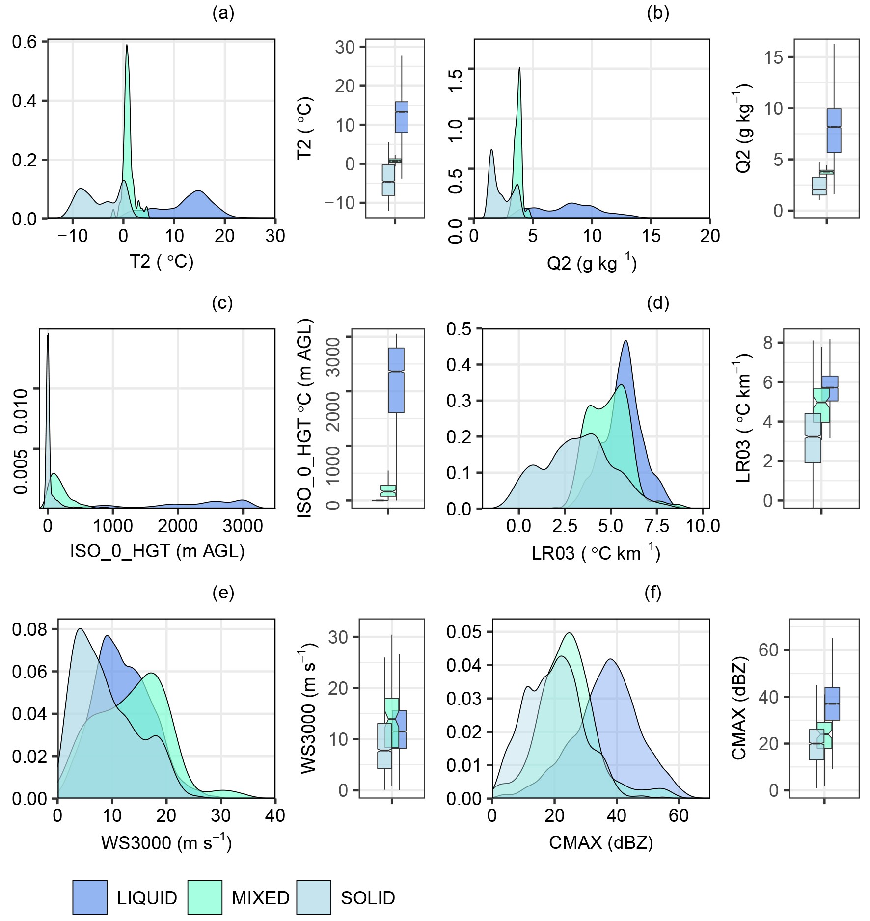
Figure 2.  Kernel Density Estimation and boxplots for selected types of precipitation (liquid, mixed and solid) according to (a) temperature at 2m AGL (T2), (b) specific humidity (Q2), (c) height of the 0°C isotherm (ISO_0_HGT), (d) 0–3 km temperature lapse rate (LR03), (e) Wind speed at 3000 m (WS3000), and (f) radar reflectivity (CMAX). The middle value on the boxplot denotes the median, with box extension from Q1 (first quartile) to Q3 (third quartile). The whiskers’ upper range is equal to Q3 + 1.5 × IQR (interquartile range), while the lower shows Q1 − 1.5 × IQR.

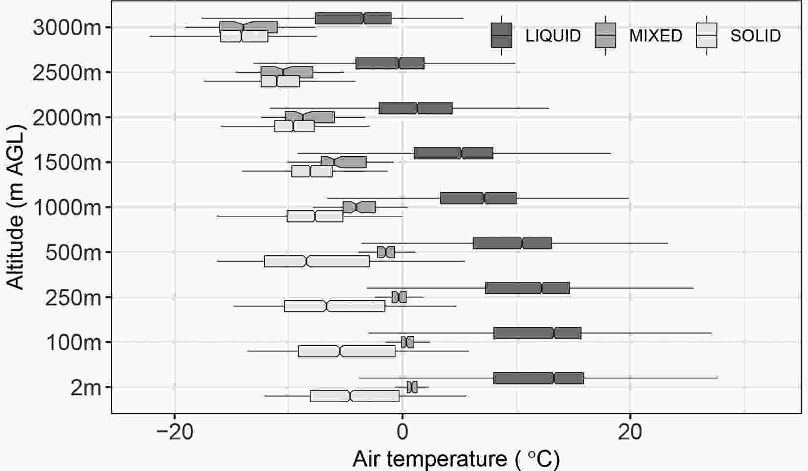
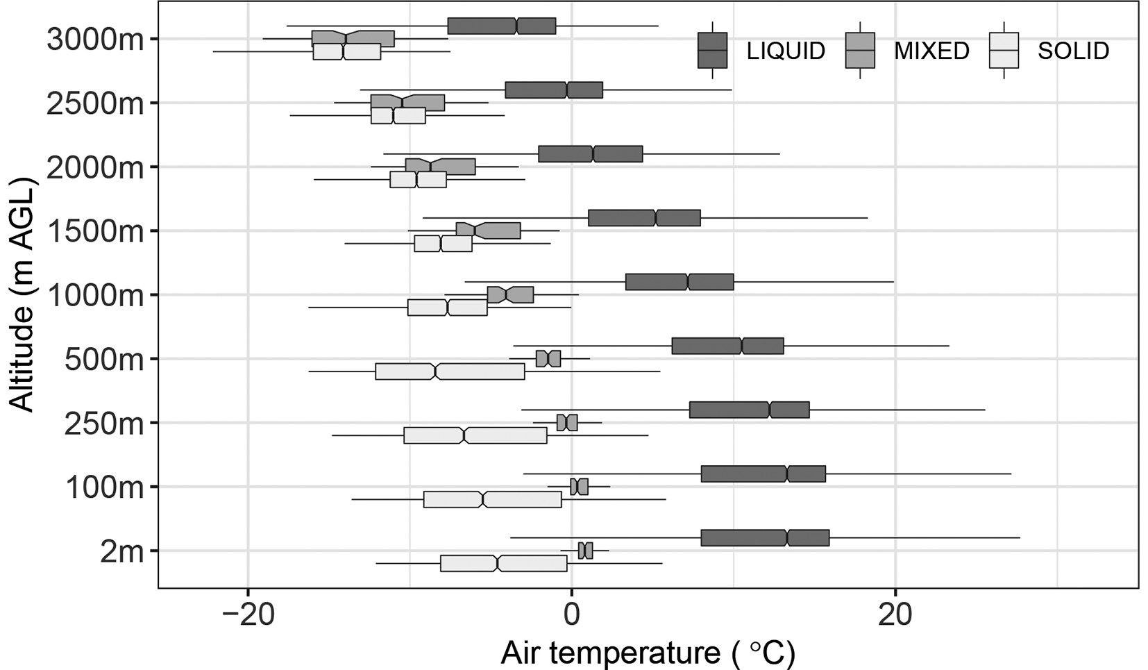
Figure 3.  Distribution of air temperature for liquid, mixed, and solid PT at selected altitudes above ground level. The details of the boxplot are the same as in Fig. 2.

The RF and the baseline classification tree (BCT) models were evaluated based on assessment of the deterministic forecast’s probability of binary events (Wilks, 2011). In the present study, the obtained probabilities of an event’s occurrence for the RF model were subsequently classified into a multi-category (3 × 3) contingency table. They show the frequency of predictions and observations in the various bins similar to scatterplots for categories. The scheme of the contingency table adopted in this study is shown in Table 2, with the observed and forecasted events split into four categories: (a) number of correct hits; (b) false alarms; (c) misses; and (d) correct rejections. In the table, n(O_i, P_j) is the number of predictions in category i that had observations in category j; N(P_i) denotes the total number of predictions in category i; N(O_j) is the total number of observations in category j, where N is the total number of forecasts.

In the case of a perfect prediction, the obtained contingency tables have non-zero elements only in the diagonal, and zero values occur only outside the diagonal. The forecast’s error measure is obtained from the off-diagonal elements of the contingency table. The marginal total of distributions (Ns on the right and at the bottom of the table) shows the accuracy of the forecast relative to the observations (Brooks and Doswell III, 1996).

Six verification measures for the contingency table were calculated to assess the robustness of the RF and BCT models. For all measures shown in Table 3, a particular PT was tested against other events. The most fundamental measures included the following: Hit Rate (H), Proportion Correct (PC), False Alarm Rate (F), and False Alarm Ratio (FAR). Moreover, it was decided to use the Critical Success Index (CSI) and Equitable Threat Score (ETS), which are more suitable for rare events, as in our case for the mixed precipitation phenomenon, which is outnumbered by solid and liquid PTs. The CSI (also called the Threat Score, TS) and ETS are used to evaluate the number of correct hits among all positive signals from the forecast of observations. The difference between the CSI and ETS (also known as the Gilbert skill score) is that the latter one additionally accounts for hits associated with random chance (Table 3), which may be more informative for imbalanced classes.

The Kernel Density Estimations (KDEs) show dependencies of the probability distribution of liquid, mixed and solid PTs as a function of air temperature, specific humidity, temperature lapse rate, wind speed, and height of the 0°C isotherm, as well as radar reflectivity (Fig. 2). These visualizations were created to help identify sharp changes in probabilities among the used variables that may potentially be applied as discriminators between the three investigated PTs.

The most remarkable factor for determination of PT is the air temperature at 2 m AGL. The shapes of the KDE curves for liquid and solid precipitation are relatively similar (broad and flat), and different from the shape of the mixed precipitation curve (Fig. 2a). The median value for the liquid PT is 13.3°C, while for mixed it is 0.8°C and for solid it is −4.6°C. Any PT may occur in a relatively narrow range of air temperature between −4.0°C and 5.6°C.

Specific humidity at an altitude of 2 m AGL (Fig. 2b) is relatively similar to the patterns in air temperature. Their median values are 8.2 g kg⁻¹ (liquid), 3.8 g kg⁻¹ (mixed), and 2.1 g kg⁻¹ (solid).

In the case of the 0°C isotherm, the distribution of probability has a significantly different shape for all considered PTs (Fig. 2c). The 0°C isotherm height for liquid precipitation ranges from 0 to 3000 m AGL (the highest level of the adopted dataset), for mixed precipitation it is from 0 to 540 m AGL, and for solid precipitation it is from 0 to about 800 m AGL. The calculated median values for the analyzed PT are 2362 m AGL for liquid, and 165 m AGL for mixed precipitation. Only in 33% of all solid precipitation cases is the 0°C isotherm located above ground level (i.e., only in those cases where the melting layer was detected). In the aforementioned 33% of analyzed solid precipitation cases, the median height is 126.3 m AGL, and the maximum value can reach even up to 791.3 m AGL. In other cases (67%), only negative air temperature values occur throughout the entire vertical profile (i.e., up to 3000 m AGL) from the ground surface.

Thermodynamic processes changing PT in a vertical aspect are often connected to the temperature lapse rate (Kain et al., 2000; Singh and Goyal, 2016), which was also taken into consideration between 2 m AGL and 3000 m AGL (Fig. 2d). The distribution is similar to the normal distribution and with better overlap compared to temperature, specific humidity and height of the 0°C isotherm. For all PTs, the lapse rate varies from −1.0°C km⁻¹ to 9.6°C km⁻¹. This means that cases with solid PT also occurred with temperature inversions. In total, 31 such situations were observed out of 2278 considered in the study. Lapse rate medians for the liquid, mixed and solid PTs are 5.7°C km⁻¹, 5°C km⁻¹ and 3.2°C km⁻¹, respectively.

Melting effects can cause pressure perturbations and can thus impact the wind field (Kain et al., 2000). Therefore, the probability distribution for wind speed at different altitudes is also investigated (Fig. 2e). However, no sharp irregularities were found as in the case of the previously described parameters. All surface PTs are possible in all wind speed ranges (from 0.1 to 33.2 m s⁻¹) at a height of 3000 m. Despite quite similar wind speed ranges in liquid, mixed, and solid PTs, their medians (11.5, 14.0 and 7.8 m s⁻¹, respectively) are different.

Among the list of variables potentially contributing to the ability of PT identification, radar reflectivity is one of the most commonly chosen products, especially for recognizing hail events (Czernecki et al., 2019). However, the robustness of this variable is not that strong if the classified PTs are grouped. The median values for liquid, mixed, and solid PTs are 37, 24 and 20 dBZ, respectively (Fig. 2f).

A clear response of the PT is visible for air temperature between 2 and 3000 m AGL (Fig. 3). Regardless of the height, the air temperature for liquid PT is the highest, and ranges on average from 13°C at 2 m AGL to −4°C at 3000 m AGL. Lower air temperature values occur for mixed PT (on average from 1°C at 2 m AGL to −14°C at 3000 m AGL), and the lowest for solid PT (on average from −5°C at 2 m AGL to −14°C at 3000 m AGL). As the height above ground level increases, the differences between categories decrease.

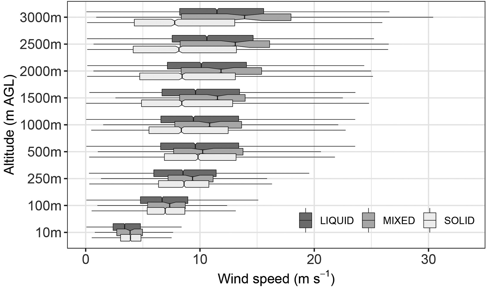
An obvious relationship can be found for the vertical profile of wind speed (Fig. 4). Above 500 m AGL, as the height increases, a slight increase in wind speed is observed for the liquid and mixed precipitation, and a decrease in wind speed for the solid precipitation. The differences in median values ​​for mixed and solid PTs are similar (especially in liquid and solid cases) for all precipitation categories of up to 500 m AGL. Above 500 m AGL, the analyzed medians of wind speeds for all precipitation categories are more diverse.

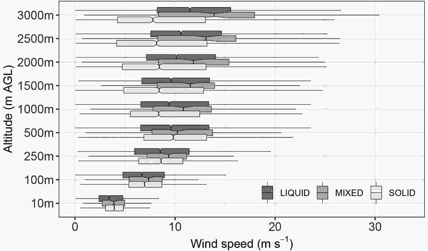
Figure 4.  Distribution of wind speed for surface precipitation types at selected altitudes above ground level. The details of the boxplot are the same as in Fig. 2.

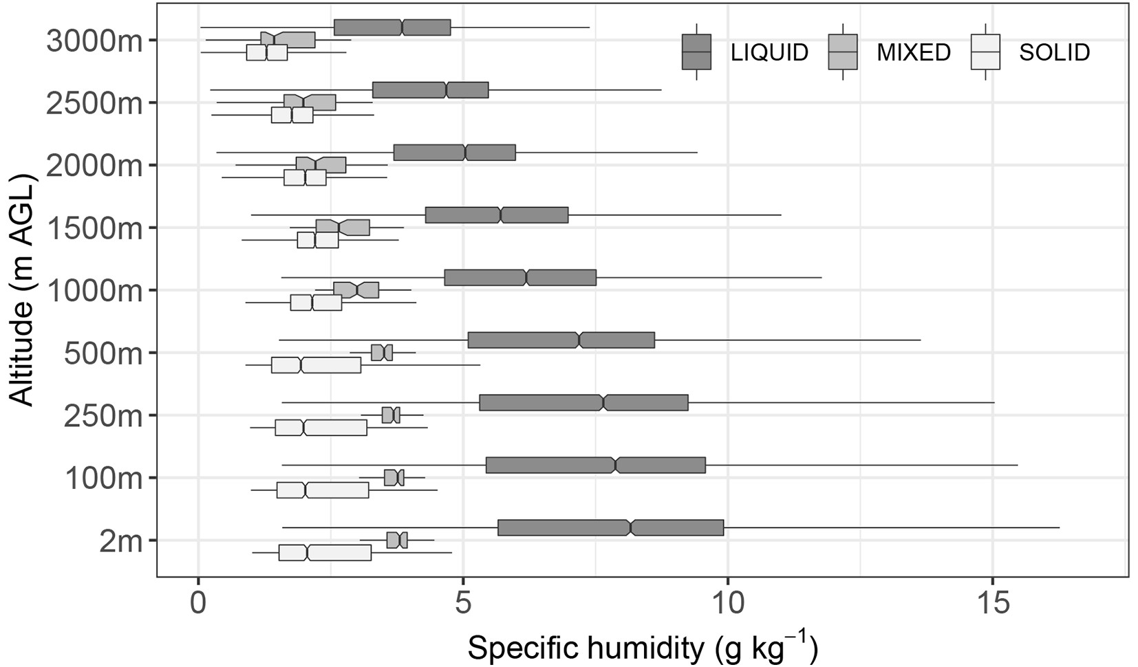
The analysis of the specific humidity ​​for individual levels indicates definitely higher humidity for liquid PT (Fig. 5). For this category, humidity drops from an average of 7 g kg⁻¹ at 2 m AGL to about 3 g kg⁻¹ at an altitude of 3000 m AGL. For mixed and solid PTs, a decrease in humidity is also observed with height, ranging from 2–4 g kg⁻¹ at 2 m AGL to about 1.5 g kg⁻¹ at an altitude of 3000 m AGL.

Figure 5.  Distribution of specific humidity for surface precipitation types at selected altitudes above ground level. The details of the boxplot are the same as in Fig. 2.

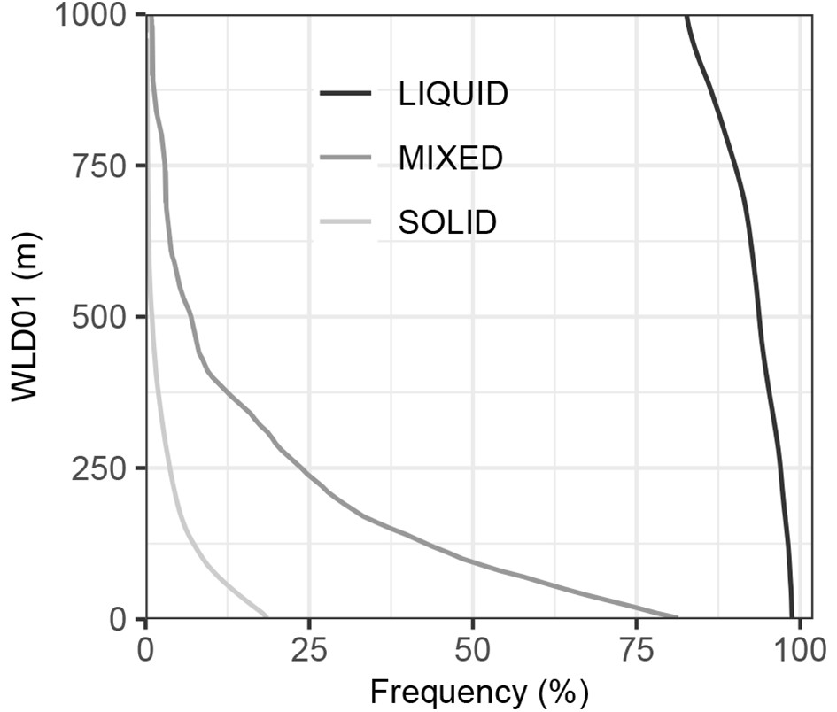
The importance of the melting effect for the determination of PT was investigated by calculating the warm layer depth with air temperature > 0°C in the range of 0–1 km AGL (Fig. 6). It was found that solid PT occurs in more than 80% of cases when the vertical profile of air temperature is above 0°C. The solid PT (i.e., ice pellets or ice crystals) may also occur when any melting layer appears above ground, which means that occurrence of such a layer is not a sufficient condition for converting solid to liquid or mixed precipitation. For the melting layer over 500 m, the frequency of solid precipitation is only 2%, while for the shallower layers the frequency of solid PT increases (12% of all cases if the melting layer is 60 m thick).

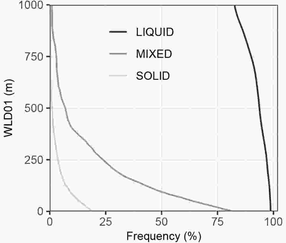
Figure 6.  Frequency of 0–1 km warm layer depth (WLD01) according to liquid, mixed and solid types of precipitation.

Atmospheric conditions accompanying mixed precipitation in the 0–1000 m AGL layer are different from those for solid PT. A quarter of the mixed precipitation occurs when the melting layer is about 250 m thick, and 50% of the cases were found when this layer reaches a thickness of about 100 m. About 20% of all cases with mixed PT can occur at a near-surface temperature below 0°C. Although the relation is clearly visible, mixed PT can occur even when the melting layer’s thickness is more than 750 m (c.a. 3% frequency) and less than a few meters. At the smallest thickness of the melting layer, the frequency of the analyzed PT is at its highest, reaching over 75%.

In turn, the conditions associated with liquid PT indicate very rare occurrences of layers with a temperature < 0°C. The vast majority of this type of precipitation (over 80% of cases) occurs when the thickness of the melting layer reaches at least 1000 m. In 95% of cases of this type of precipitation, the melting layer is 500 m thick, and in 98% of cases it reaches 250 m.

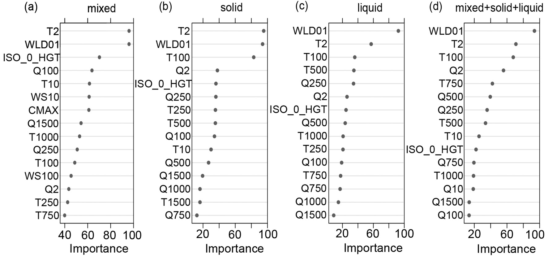
Considering the KDE values (Fig. 2) it can be assumed that some parameters might be used as robust covariates in modeling PT. The scaled variable importance of predictors used in the RF models are shown together in Fig. 7. Given the contribution of the variable importance to the RF models, it can be seen that values may differ for individual models, although some of them, e.g., T2 or WLD01, are in each case one of the leading factors. This is due to the complexity of the physical processes of forming liquid, solid or mixed PTs, as well as the properties of the chosen ML algorithm. To distinguish mixed PT from liquid PT, T2 is the dominant discriminator, while for liquid precipitation T2 is the second most important after the depth of the melting layer, which justifies adding this variable to the ML model setup.

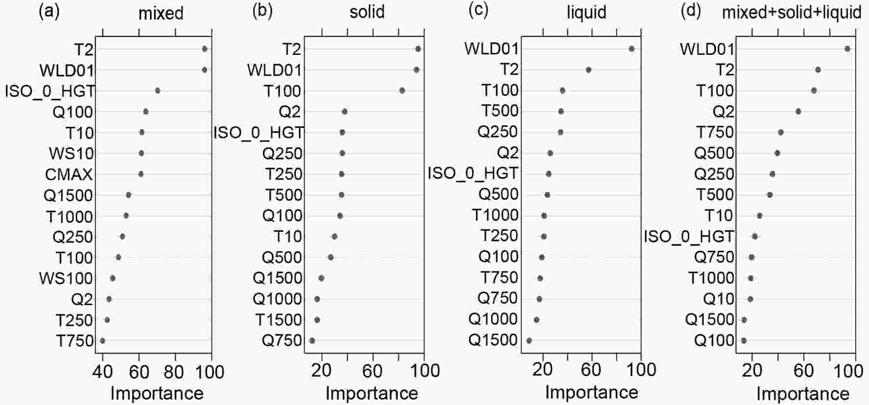
Figure 7.  Variables’ importance of predictors (0–100 scaled) applied in the RF models for (a) mixed, (b) solid, (c) liquid, and (d) all PTs.

It is worth noting that the RF model indicated significance of the wind speed parameters in the vertical profile (WS10, WS100) for the mixed PT only, along with a high impact of the 0°C isotherm height. In the case of liquid and solid PTs, the created model was based mostly on humidity parameters. Low importance was detected for CMAX radar reflectivity, which was only used by decision trees to determine mixed PTs.

We also tested how the variables’ importance changes if all factors and all PTs are used simultaneously (Fig. 7d). As it turned out, the most important predictor is WLD01, and the other predictors giving a significant signal for modeling PT are: T2, T100, Q2, then T750, Q500, Q250, and T500. Other covariates with lower importance (i.e., T10, ISO_0_HGT, Q750, T1000, and Q10) seem to slightly improve the model parameters.

The contingency table of observed and predicted PTs (Table 4) is computed for the benchmark model and most generic RF models that rely on using all meteorological predictors for classifying all PTs simultaneously. Table 5 presents the results relating to performance measures derived from the contingency table. For all analyzed cases, the RF model obtained better verification scores than the developed BCT model. Moreover, the differences between models were significant according to the p-value statistics obtained from the t-test, confirming a clear improvement while applying ML algorithms together with the data fusion approach.

The best evaluation measures were obtained for liquid PT, which occurred most frequently. In this case, among all observed 1091 cases, the RF model correctly predicted 1066, giving a high H of 0.980. For the unsuccessful cases of liquid PT, the model incorrectly indicated solid (13 cases) and mixed (14 cases) PT instead of liquid, which in total gave a slightly overestimated result (1093 forecasted cases). Hence, the F (also called Probability of False Detection, or POFD), which is conditioned on observations rather than forecasts, was 0.023. The number of false alarms described by the FAR was similar (0.025). Therefore, it is unsurprising that the CSI and ETS for liquid PT reached a high level of 0.956 and 0.917, respectively. Moreover, as the ETS indicator shows, the RF model detects liquid PT much better than the BCT model (0.655). Furthermore, the RF model’s better performance is especially noticeable with the reduced number of false alarms.

For the solid PT among all observed 1077 cases, the model correctly predicted 1062, giving a similarly high H value of 0.988. Among the incorrectly forecasted cases of solid PT, the model indicated mostly liquid (22 cases) as well as mixed (18 cases) PT, giving an overestimated result of 1102 forecasted solid PTs. For solid PT, the probabilities of the F and the FAR were the highest among all PTs, reaching a level of 0.034 and 0.036, respectively. Similar to liquid PT, in the case of solid PT, the CSI and ETS reached a high level of 0.953 and 0.911, respectively. Comparing the ETS values for RF and BCT, a large difference is noticeable (91.1% for RF and 65.1% for BCT), indicating a much better performance of the RF model.

Considering the mixed PT for all observed 98 cases, the model correctly predicted 66 cases giving the lowest H value (0.673). The incorrectly forecasted mixed PT deals with only five unsuccessful cases, when instead of mixed, the model predicted three liquid and two solid PTs. This means that the model underestimates the forecast for the mixed PT, and hence the F and the FAR were both 0.0. Different from the liquid and solid precipitation, in the case of the mixed PT, the CSI and ETS had their lowest values of 0.673 and 0.664, respectively. CSI and ETS are especially valuable when observed values are not frequent (mixed PT); their sensitivity towards taking into account both false alarms and missed events makes them more balanced scores than, for example, the H. However, because the mixed PT was unsuccessfully predicted only five times here, both measures (H and CSI) indicated the same value. Similar to the liquid and solid PT, for the mixed type, the ETS values indicate significantly greater robustness for the RF model than for the BCT one (66.4% and 10.7%, respectively).

The use of ML techniques provides the possibility of more accurate forecasts in areas where NWP models tend to be less skillful (Brimelow et al., 2002; Gagne et al., 2017; Dennis and Kumjian, 2017). It is particularly visible in microphysical and convective processes, which usually cannot be computed implicitly and therefore need to be parameterized (Allen et al., 2015; McGovern et al., 2017; Gagne et al., 2017; Ukkonen et al., 2017). Therefore, it has become increasingly common to use ML algorithms for identifying the most skillful variables in predicting specific types of weather phenomena.

In the present study, the data fusion approach using the RF technique was applied. The surface synoptic observations and ERA5 reanalysis, as well as radar data for predicting three PTs—namely, liquid, solid and mixed—were used. Using these methods and data, an attempt was made to answer the question: “How can ML techniques applied in observational and NWP data help to improve the recognition of the surface PT?”

The created generic model distinguishes PTs based mostly on the depth of the melting layer and the near-surface air temperature. The depth of the melting layer proved to be a very good predictor of the PT, which allowed us to conclude that, in 95% of all cases with liquid PT, the melting layer was > 500 m deep (in 98% of cases, this layer was > 250 m deep). Together with changes to the specific humidity in the vertical profile, it brings forth the largest signal in a proper identification of PT (Fig. 7d), which confirms that analysis of the vertical distribution of temperature and humidity is the key ingredient to a successful modeling of PTs (Gjertsen and Ødegaard, 2005; Thériault et al., 2010; Schuur et al., 2012; Ding et al., 2014; Reeves et al., 2016).

Attention should also be paid to the relationship between the higher wind speed at the height above 10 m AGL and the occurrence of mixed precipitation (Fig. 4). For the mixed PT, the wind speed ranks sixth (10 m AGL) and twelfth (100 m AGL) among the variables’ importance. For liquid and solid PTs, the wind speed does not appear among the first fifteen predictors.

The probability density estimation of the radar reflectivity (CMAX) for the conditional probability of the liquid, mixed and solid precipitation (Fig. 2) can be assumed to have high importance in recognizing the PT. However, the obtained results indicate that this is not the case for grouped classes of PT. As an important variable, the CMAX value signal was only indicated by the RF model in the case of the mixed PT. However, as indicated by the KDE distribution, the high values of CMAX (> 45 dBZ) demonstrate a potential to distinguish between liquid and other PTs as it is typically a rare situation for either solid or mixed PT to reach such a high reflectivity value. However, contrary to our findings, it should also be pointed out that Gjertsen and Ødegaard (2005), in their study of rainfall recognition during the winter season in Norway, used radar data as input variables and demonstrated their usefulness. Schuur et al. (2012) demonstrated the potential benefits of combining polarimetric radar data with thermodynamic information from the RUC (Rapid Update Cycle) model. According to Czernecki et al. (2019), applying ML techniques as well as the data fusion approach indicated CMAX to be a good predictor for large hail recognition. Therefore, it must be kept in mind that CMAX itself is a robust predictor for determining any precipitation occurrence, which admittedly was not the scope of our study where only situations with precipitation are considered. Therefore, even without the CMAX product, the developed RF model delivered more reliable classification results to date than other methods.

The obtained classification results are most promising for liquid and solid PTs, while mixed types are the most challenging. This should not be a surprise, as the classification of these phenomena may even vary among different station observers and thus may also impact the quality of input data. Forecasting of mixed precipitation is markedly more difficult than that of solid or liquid PT, as already stated in earlier studies (Kain et al., 2000). In the present study, the H value for liquid precipitation was 98.0% (1066 out of 1091 cases), while for solid precipitation it was 98.8% (1062 out of 1077 cases) and for mixed it was 67.3% (66 out of 98 cases) PTs. The F values were highest for solid precipitation (0.034), lower for liquid precipitation (0.0023), and lowest for mixed (0.000). Although a comparison of values may be challenging (or even impossible in many cases due to different evaluation indices, environmental circumstances, observational techniques, and the applied precipitation classification), the evaluation metrics clearly indicate the robustness of the ML approach, especially if compared with other NWP-based studies.

PT forecasts that took into account a division into different water phase types (e.g., rain, sleet, snow) from the HIRLAM (High Resolution Limited Area Model; Undén 2002), based on synoptic observations and weather radar data, was presented by Gjertsen and Ødegaard (2005). In this study, the obtained results of PT detection were 84% for rain and 97% for snow. Reeves et al. (2016), based on spectral-bin microphysical modeling for recognizing rain and snow in the winter season, obtained POD (Probability of Detection) values at a level of 91.4% to 98.3%. However, this comparison can only be done in a very generic way because a more detailed breakdown of PT was applied, not to mention that this study covered a relatively narrow range of air temperature that could not be used as a robust predictor. In turn, the proposed RF model gives much better results compared to the basic BCT. For each PT, all the performance measures indicate a significantly better robustness of the RF model, in particular for mixed PT, which is the most difficult to forecast.

The application of ML techniques and the data fusion approach in predicting different PTs brings to the fore a promising concept for future application as a post-processing tool that might easily be combined with operationally used NWP models. It may become especially useful during the winter season when a proper recognition of PT might reduce the risk of hazards in transportation, and thus may prevent adverse socioeconomic impacts (Gjertsen and Ødegaard, 2005; Ikeda et al., 2013).

Acknowledgements. This research was supported by grants from the Polish National Science Centre (project numbers 2015/19/B/ST10/02158 and 2017/27/B/ST10/00297). The computations were partly performed in the Poznań Supercomputing and Networking Center (Grant No. 331). We would like to thank the Polish Institute of Meteorology and Water Management – National Research Institute, for providing the radar-derived products.