


 DownLoad:


HTML
-
As a critical biogeochemical process, the nitrogen cycle involves the circulation of nitrogen among the atmospheric, terrestrial, and marine ecosystems. As a nutrient, nitrogen constrains vegetation carbon assimilation and plant growth (Fisher et al., 2012), which then impacts the hydrological cycle through plant transpiration (Liu et al., 2013).
Human activities have significantly modified the terrestrial nitrogen cycle (Vitousek et al., 1997; Erisman et al., 2013) and resulted in a plethora of environmental issues. Nitrogen fertilizer, as a typical example, is intensively applied in agriculture, which has increased dramatically in recent decades, accounting for half of the total nitrogen input to soil (i.e., fertilizer application, atmospheric deposition, and biological nitrogen fixation) (Fowler et al., 2013), especially in developing countries such as China. Excessive nitrogen fertilizer leaches into water bodies, causing eutrophication (Boesch et al., 2009; Conley et al., 2009), and releases ammonia gas into the atmosphere, causing air pollution (Suddick et al., 2013).
Land surface models (LSMs) quantitatively represent the complex interactions among the terrestrial nitrogen, carbon, and water cycles (Dickinson, 1991; Pitman, 2003) and are a vital tool to address the impacts of the natural variations of nitrogen availability and human perturbations on the environment. In recent years, several LSMs have represented the terrestrial nitrogen cycle, such as the augmented Integrated Science Assessment Model (Yang et al., 2009). Koven et al. (2013) and Shi et al. (2016) incorporated the impacts of nitrogen availability on the carbon cycle (CN) into the widely used Community Land Model (CLM). Their evaluations using site-level and global datasets exhibited good performances in modeling carbon balance and net primary production (NPP), but region-specific evaluations are still lacking, especially with regard to the environmental issues.
Incorporating the terrestrial nitrogen cycle into the Noah LSM with multi-parameterization options (Noah-MP) (Niu et al., 2011) is particularly appealing. Noah-MP has been coupled with the Weather Research and Forecasting (WRF) model (Barlage et al., 2015) and the National Water Model (NWM) (Maidment, 2017). WRF is widely used for high-resolution regional weather and air pollution forecasts (Barlage et al., 2015), and NWM is currently operational at the National Oceanic and Atmospheric Administration for nationwide streamflow forecasts over the continental United States. A regionally applicable nitrogen-augmented Noah-MP LSM would enable modeling studies of the impacts of fertilizer use on air and water pollution.
Noah-MP has been broadly evaluated in representing regional terrestrial carbon and water cycles (Cai et al., 2014; Ma et al., 2017; Lin et al., 2018; Liang et al., 2019). Cai et al. (2014) compared Noah-MP with the Variable Infiltration Capacity model, Noah, and CLM using the North American Land Data Assimilation System testbed and showed that Noah-MP performed the best in reproducing observed soil moisture. Lin et al. (2018) evaluated Noah-MP-simulated streamflow and showed its potential in enhancing the hydrological forecasting capability. Ma et al. (2017) evaluated the dynamic vegetation parameterization of Noah-MP over the continental United States. They showed that, with dynamic vegetation, Noah-MP successfully simulated net radiation, runoff and snow-cover fraction, but overestimated gross primary productivity (GPP) significantly and evapotranspiration (ET) moderately. They also suggested that incorporating dynamic nitrogen constraints may be a worthwhile method to correct the biases in GPP and ET.
Recently, Cai et al. (2016) incorporated the dynamic nitrogen constraints on photosynthesis into Noah-MP (hereafter referred to as Noah-MP-CN). Noah-MP-CN is lightweight and easy to operate in comparison to CLM-CN, but can reasonably reproduce the in-situ observed carbon and water cycles (Cai et al., 2016). However, the model has only been evaluated on the plot scale, and its performance in modeling regional-scale terrestrial water, carbon and nitrogen cycles is still unknown. Several difficulties exist in extending simulations from the plot scale to the regional scale. First, it has not been explored how the model parameters can be derived for different land-cover and land-use types. Second, collecting and processing soil texture−related datasets for the soil nitrogen module require tremendous efforts. Third, regional validation data are limited, especially for nitrogen-related variables such as soil nitrogen content.
By taking on the above challenges, this paper presents the first application of the nitrogen-augmented Noah-MP-CN on the regional scale. Section 2 describes the development of the regional-scale Noah-MP-CN by utilizing spatially varying parameters and inputs. Section 3 introduces the observational data and the simulation settings over China, a country with the largest amount of nitrogen fertilizer application. The modeled terrestrial water and carbon cycles are comprehensively evaluated. Sensitivity analyses with different amounts of fertilizer application are conducted, providing in-depth analyses of how water consumption and carbon fixation are affected by nitrogen availability. The evaluations and sensitivity analyses are detailed in section 4, followed by conclusions in section 5.
-
Noah-MP improves over the Noah LSM (Niu et al., 2011; Yang et al., 2011) by including a short-term dynamic vegetation scheme (Dickinson et al., 1998), a modified two-stream radiation transfer scheme (Yang and Friedl, 2003; Niu and Yang, 2004), TOPMODEL-based runoff and groundwater schemes (Niu et al., 2005, 2007), and a more permeable frozen soil scheme (Niu and Yang, 2006).
Noah-MP hosts multiple parameterization options for several major physical processes, including vegetation phenology, canopy stomatal resistance, runoff, groundwater, and soil moisture limitation to transpiration (Niu et al., 2011; Yang et al., 2011). In order to incorporate nitrogen dynamics into Noah-MP, the dynamic vegetation option [instead of commonly used static climatological leaf area index (LAI) values] has to be enabled to update plant biomass and LAI based on photosynthesis. Other options are the same as the settings used in the site-evaluation experiment by Cai et al. (2016), which are recommended options in this version of Noah-MP [shown in Table S1 in electronic supplementary material (ESM)]. Nitrogen availability constrains the rate of photosynthesis. The constraint is induced by a foliage nitrogen factor parameter (Running and Coughlan, 1988) and is currently static in Noah-MP (the version without the dynamic nitrogen module). The foliage nitrogen factor adjusts the calculation of the maximum rate of carboxylation (Vmax), a factor controlling the total carbon assimilation rate, shown in Eq. (1):
where Vmax25 is the maximum carboxylation rate at 25°C (μmol CO2 m−2 s−1), αvmax is a temperature-sensitive parameter, f(Tv) is a function that mimics the thermal breakdown of metabolic processes, and β is the soil moisture controlling factor. The term fNIT, less than 1, is a foliage nitrogen factor, which is always set as a constant (0.67), indicating that a 33% reduction in Vmax is due to the limitation of nitrogen.
-
The static nitrogen constraint of Noah-MP is augmented by incorporating plant nitrogen dynamics based on the Fixation and Uptake of Nitrogen (FUN) model (Fisher et al., 2010) and soil nitrogen dynamics based on the Soil and Water Assessment Tool (SWAT) (Neitsch et al., 2011). The resultant Noah-MP-CN (Cai et al., 2016) is different from CLM-CN in that the former focuses on short-to-medium-range weather and environmental forecasts, while the latter targets long-term climate assessments. The FUN model was adopted in Noah-MP-CN because it uses the advanced carbon cost theory in plant nitrogen uptake, and SWAT was chosen for its strength in agricultural management and water-quality modeling. Specifically, FUN models plant nitrogen uptake and its carbon cost (NPP reduction), and there are four plant nitrogen uptake pathways: passive (advection with soil moisture being the medium) and active soil nitrogen uptake, symbiotic biological nitrogen fixation, and leaf nitrogen retranslocation. SWAT separately models the mineral and organic forms of soil nitrogen through the interactions between them via processes such as atmospheric deposition and leaching. The model flow chart and detailed mathematical formulations of the processes can be found in Cai et al. (2016).
Model parameters are the same as those used in Cai et al. (2016), except the following differences adjusted for regional simulations (shown in Table S2 in the ESM). The scaling factor of the symbiotic biological nitrogen fixation process and the threshold value of the soil water factor for denitrification to occur have been found to be two sensitive parameters (Cai et al., 2016). In this study, these two parameters are set for each land-use/land-cover type, and their values are shown in Table 1 to represent our best guesses based on the literature suggesting the default values of these parameters and our own experience. Some input parameter datasets, whose sources are shown in Table 2, are spatially varying (i.e., values vary based on location or by certain soil types or land-use/land-cover types), and they were collected by this study. Specifically, the soil-texture-related parameters, provided by Wei et al. (2014), were downscaled from their original resolution to 0.25° to be consistent with the model. The slope steepness and length factors of the Universal Soil Loss Equation (ULSE) were obtained from the National Science & Technology Infrastructure of China with interpolation. Based on the classification of the global land-cover database for the year 2000 (GLC 2000), we obtained the USLE support practice factor. According to the equation from Sharpley et al. (1993), the ULSE erodibility factor was calculated based on the soil texture attributes.
Parameter s γsw,thr Cropland −40 0.91 Forest −6.25 0.91 Grassland −30 0.85 Savannas −40 0.85 Shrublands −6.25 0.85 Others −6.25 0.85 Table 1. Major sensitive parameters based on our own experience. s is the scaling factor. γsw,thr is the threshold value of soil water factor for denitrification to occur.
Definition Source Soil bulk density Wei et al. (2014) Available water capacity of the soil layer Wei et al. (2014) Organic carbon content Wei et al. (2014) Clay content Wei et al. (2014) Silt content Wei et al. (2014) Sand content Wei et al. (2014) Rock content Wei et al. (2014) Fraction of porosity from which anions are excluded Default: 0.15 USLE slope steepness (S) factor National Science and Technology Infrastructure of China USLE slope length (L) factor National Science and Technology Infrastructure of China USLE support practice (P) factor GLC2000 USLE soil erodibility (K) factor Sharpley et al. (1993) Table 2. Soil input data.
The nitrogen module requires two inputs: atmospheric nitrogen deposition and nitrogen fertilizer use. The atmospheric deposition is divided into wet and dry deposition, which are calculated by empirical formulae (Neitsch et al., 2011). The global fertilizer dataset, including the amount of nitrogen fertilizer of a year, provides the model inputs. The dataset does not have the fertilizer application date. We chose 1 June as the fertilizer application date according to previous point-scale work (Cai et al., 2016) because it is in the middle of the growing season. Note that this choice might be a source of uncertainty because the fertilizer application date varies spatially according to crop type. More comprehensive fertilizer-use datasets with detailed application dates are desirable in future work.
2.1. Noah-MP
2.2. Noah-MP-CN for regional applications
-
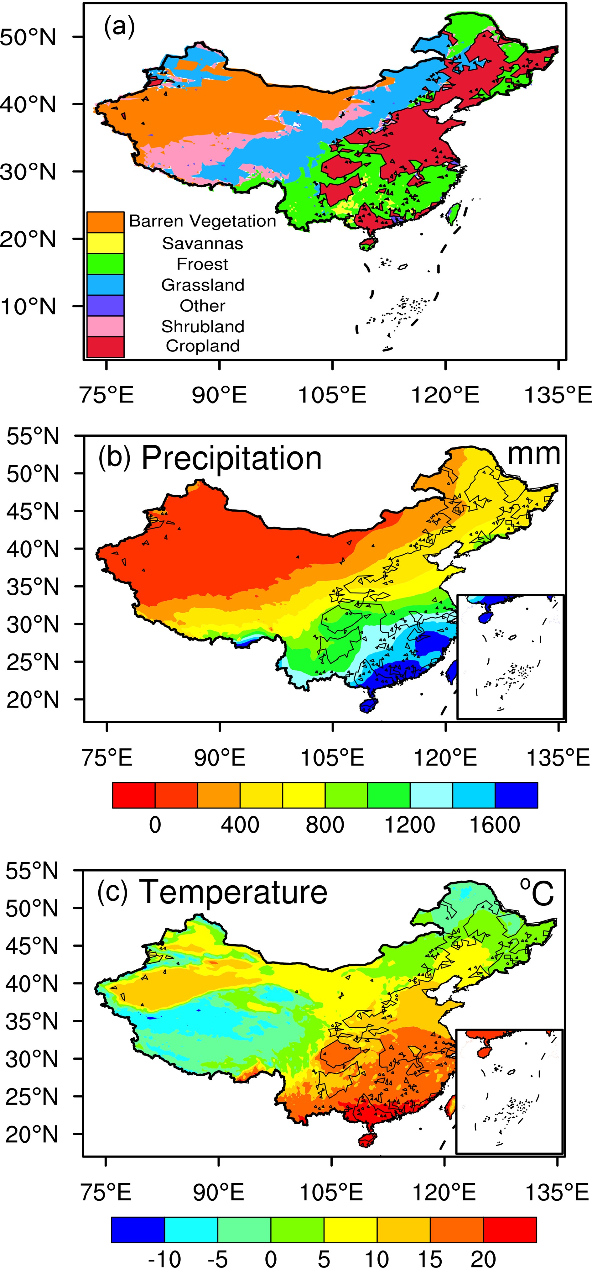
We chose China as our testbed for the regional application of Noah-MP-CN, which covers an area of 9.6 million km2, with considerable climate variation and various land-use/land-cover types. During the study period (2001−14), the average annual temperature is 7.68°C and the annual total precipitation is 720 mm, both of which show clear northwest to southeast gradients (Fig. 1) and very good spatial correspondence with different land-use/land-cover types. In addition to the whole country scale, we also focus our model evaluation efforts on croplands because fertilizer application globally contributes to ~50% of the total nitrogen input to the soil (Fowler et al., 2013). Moreover, croplands are a major source of nitrogen loading in water bodies, which has significant impacts on the environment, so it is evaluated with particular scrutiny in this study.

Figure 1. Map of China showing (a) land use and land cover, and average annual (2001−14) (b) precipitation and (c) temperature. The lines in (a) delineate the distribution of cropland in China.
-
We used NASA’s Global Land Data Assimilation System (GLDAS) (Rodell et al., 2004), version 2.1, meteorological data to drive the model. The forcing data were derived by combining atmospheric reanalysis, remote sensing, and ground observations. The spatial resolution is 0.25° and the temporal resolution is 3 h. There are other forcing datasets, including the dataset provided by the China Meteorological Administration (Meng et al., 2017). However, GLDAS is chosen for two reasons. First, the performance is sound. Our previous study (Liang et al., 2019) found that using GLDAS v2.1 for the same domain, Noah-MP simulates water budget components well. Second, GLDAS has the potential to be used in global simulations.
-
When coupled with the nitrogen module, soil attributes are key input datasets. As listed in Table 2, we obtained the bulk density, available water capacity, and organic carbon, clay, silt, sand, and rock content from the gridded Global Soil Dataset for use in Earth System Models (GSDE) (Wei et al., 2014). GSDE was generated based on the soil map of the world and various regional and national soil databases, including soil attribute data and soil maps, at a resolution of 30 arc-seconds (about 1 km at the equator). The vertical variation of soil properties in this dataset was captured by eight layers to the depth of 2.3 m (i.e., 0−0.045, 0.045−0.0901, 0.091−0.166, 0.166−0.289, 0.289−0.493, 0.493−0.829, 0.829−1.383 and 1.383−2.296 m), which were interpolated into four soil layers (i.e., 0−0.1, 0.1−0.4, 0.4−1.0 and 1.0−2.0 m) to be consistent with the model setup. The factors of the USLE were based on the Loess Plateau Data Center, National Earth System Science Data Sharing Infrastructure, National Science & Technology Infrastructure of China (http://loess.geodata.cn). Besides, GLC2000 (Bartholomé and Belward, 2005) and the equation from Sharpley et al. (1993) were also used to estimate the USLE factors. To be consistent with the resolution of the forcing data, the entire soil attribute dataset is bilinearly interpolated to 0.25°.
-
The amount of nitrogen fertilization is an important input to the nitrogen module. The global dataset of annual nitrogen fertilizer employed (Lu and Tian, 2016) was based on surveys of country-level fertilizer inputs collected by the IFA (International Fertilizer Industry Association) and FAO (Food and Agricultural Organization). It has a spatial resolution of 0.5°, covering 1961−2013. Here, we select the data for the period 2001−13.
-
The Global Land Surface Satellite (GLASS) dataset provides an LAI product with a long time series and high level of precision, which is derived from Moderate Resolution Imaging Spectroradiometer (MODIS) land surface reflectance data (MOD09A1) and released by the Center for Global Change Data Processing and Analysis of Beijing Normal University (Liang et al., 2013; Xiao et al., 2014). It is provided in a geographic projection of the Climate Modeling Grid at a high spatial resolution of 0.05° and a temporal resolution of eight days. Due to its reliability, spatial integrity, and temporal consistency, this product has been used in a range of applications (Xiao et al., 2016; Zhang et al., 2016) in global change and climate studies, especially showing its advantages in our domain among other remotely sensed datasets (Li et al., 2018), which gives us confidence to use it as evaluation data in the present study.
-
The GPP monthly data were obtained from FLUXCOM (Jung et al., 2011) and MODIS (Zhao et al., 2005). Based on 224 FLUXNET sites, the global GPP dataset is obtained, at a spatial resolution of 0.5° and a temporal resolution of monthly during the period from 2001 to 2013, and the ensemble mean of the total dataset is used here. MODIS GPP is available from the Numerical Terra Dynamics Simulation Group at the University of Montana. MOD17A2 has a spatial resolution of 0.05°, covering the period 2000−15, and the data from 2001−13 are used as one of the validation datasets. Considering the advantages and widespread use of MODIS (Zhao et al., 2005) and FLUXCOM (Jung et al., 2017), we use the mean of these two datasets as the validation data to eliminate the possible existence of observational errors.
-
Based on the remote sensing data provided by NASA’s Terra and Aqua satellites, Jung et al. (2011) generated global MODIS ET datasets (MOD16) with an improved algorithm, which have subsequently been used for different applications in science and management, such as calculating energy and water balances. The dataset is available for the entire global vegetated land area at eight-day, monthly and annual intervals, with a spatial resolution of 1 km. We use the MOD16A2 monthly ET dataset (covering the period 2001−11) as model validation data.
-
The observed soil moisture data were provided by the Chinese Crop Growth and Farmland Soil Moisture Dataset of the China Meteorological Administration’s Science Data-sharing Network (
https://escience.org.cn/ ). Observations were routinely measured in the warm season (March−November) every 10 days (usually on the 8th, 18th and 28th of the month). The cold-season observational data are not used here due to the freeze−thaw state of soil and quality assurance. The depth of observation mostly ranges from 10 cm to 100 cm with the units in relative humidity. Considering the availability of observations and matching with the simulation results, we only compare the soil moisture at the depth of 10 cm after converting the units to volumetric water content. Although its spatial and temporal resolution are relatively low, this soil moisture dataset is currently the most extensive in terms of spatial coverage in China and has the longest observational period, part of which was integrated into the global soil moisture database produced by Robock et al. (2000). Therefore, we consider this dataset a reliable data source for evaluating LSMs. To ensure comparability and avoid continuity problems caused by missing values, we choose 2001−11 as the analysis period. -
The metrics used for evaluating the model are the correlation coefficient (R) and root-mean-square error (RMSE), which are calculated as follows:
where Mi and Oi denote the simulation and observation values, respectively; and
$\bar M$ and$\bar O$ denote the mean of the simulation and observed values, respectively. -
We conducted two experiments with the Noah-MP and Noah-MP-CN model respectively, assessing the impacts of the static and dynamic nitrogen constraints on photosynthesis as shown in Eq. (1): Noah-MP uses a static foliage nitrogen parameter, whereas Noah-MP-CN models the soil and plant nitrogen dynamics and represents the dynamic constraints of nitrogen availability on photosynthesis. At the beginning of each experiment, we repeat the simulation by using the forcing of 2000 for 200 times to reach model equilibrium, and the output for the last time step is used as model initialization for both experiments to obtain the modeling results of the period between 2001 and 2014.
Nitrogen fertilizer use can significantly influence nitrogen availability. Based on the above-described Noah-MP-CN experiment (denoted FT3) with the actual fertilizer application amount, two additional experiments with halved fertilization (denoted FT2) and without fertilization (denoted FT1) are conducted to investigate the sensitivity to the different amounts of fertilizer application.
3.1. Domain
3.2. Data
3.2.1. Model input data
3.2.1.1. Meteorological data
3.2.1.2. Soil input data
3.2.1.3. Fertilizer input data
3.2.2. Evaluation data
3.2.2.1. LAI
3.2.2.2. GPP data
3.2.2.3. ET data
3.2.2.4. Soil moisture data
3.3. Evaluation metrics


3.4. Model experiments
-
LAI is defined as the one-sided green leaf area per unit ground surface area. LAI is a controlling factor of major biophysical processes including photosynthesis, respiration, ET, and the carbon cycle.
Figure 2 compares the multi-year mean LAI between simulations and GLASS. Both Noah-MP and Noah-MP-CN capture the observed spatial pattern, which exhibits an obvious gradient increasing from northwest to southeast. Noah-MP overestimates LAI in most regions, especially in the southern areas. This assessment is consistent with that by Ma et al. (2017) over the continental United States. The overestimation is reduced to some extent in Noah-MP-CN. The improvements from considering nitrogen constraints on carbon are more obvious in terms of temporal correlation. Similar to the assessment of the multi-year mean values, the improvements in temporal correlation are also mainly located in southeastern China, where both Noah-MP and Noah-MP-CN show relatively reasonable correlations with GLASS. Including the limitation of nitrogen on carbon assimilation also reduces the RMSE of the simulated LAI, and these RMSE decreases are observed in almost the entire domain.
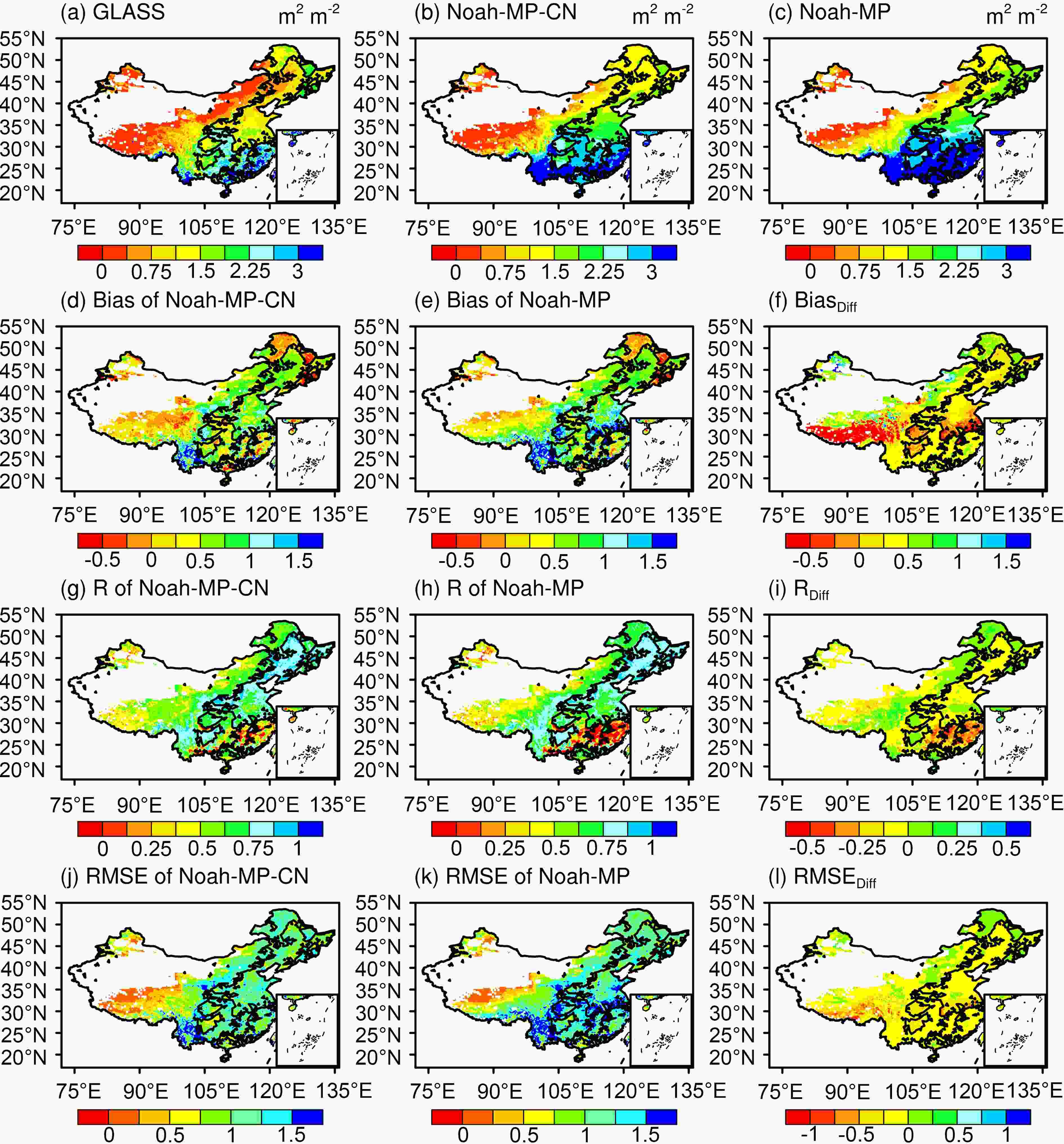
Figure 2. Spatial distribution of multi-year averaged LAI (m2 m−2) during 2001−14 for (a) BNU_GLASS, (b) Noah-MP-CN, and (c) Noah-MP. Bias of LAI during 2001−14 (d) between Noah-MP-CN and BNU_GLASS, (e) between Noah-MP and BNU_GLASS, and (f) Noah-MP-CN minus Noah-MP in the relative absolute LAI biases. Relative absolute LAI biases are defined as the absolute biases between modeled LAI and GLASS LAI, divided by GLASS LAI. Correlation coefficients of LAI during 2001−14 (g) between Noah-MP-CN and BNU_GLASS, (h) between Noah-MP and BNU_GLASS, and (i) Noah-MP minus Noah-MP-CN. RMSE of LAI during 2001−14 for (j) Noah-MP-CN, (k) Noah-MP, and (l) Noah-MP-CN minus Noah-MP.
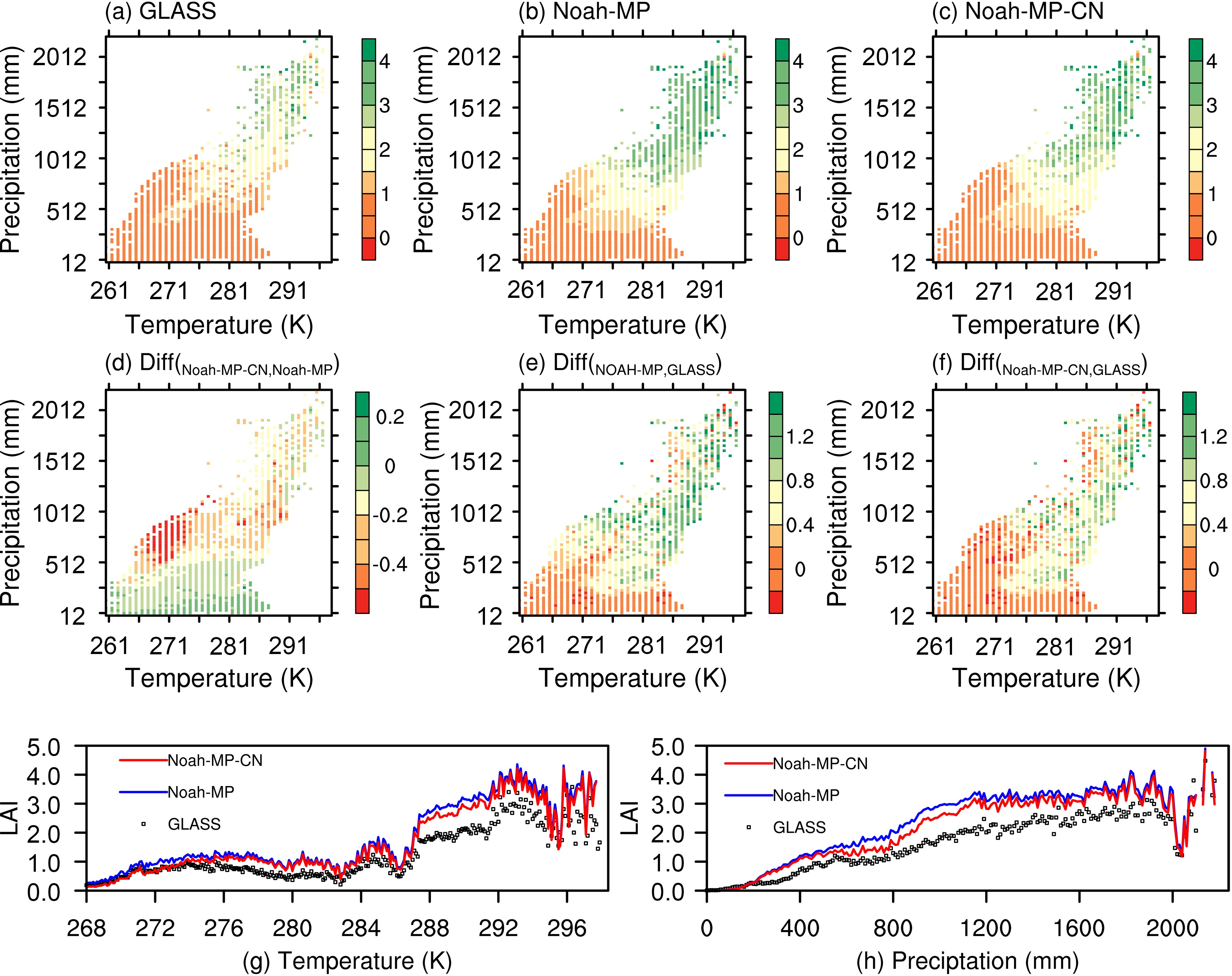
Figure 3 compares the simulated multi-year mean LAI from Noah-MP and Noah-MP-CN in different climatic zones, which are characterized by multi-year-averaged temperature and annual precipitation, two important climatological factors in determining vegetation distribution and growth. Figures 3g and h show that Noah-MP captures the dependency of LAI on temperature and precipitation well, but with a positive bias. Noah-MP-CN reduces the biases of Noah-MP. Figures 3a-f show that the bias reduction of Noah-MP-CN mainly exists in the relatively humid and warm regions, where the multi-year-averaged annual precipitation is more than 800 mm and the temperature is over 281 K.
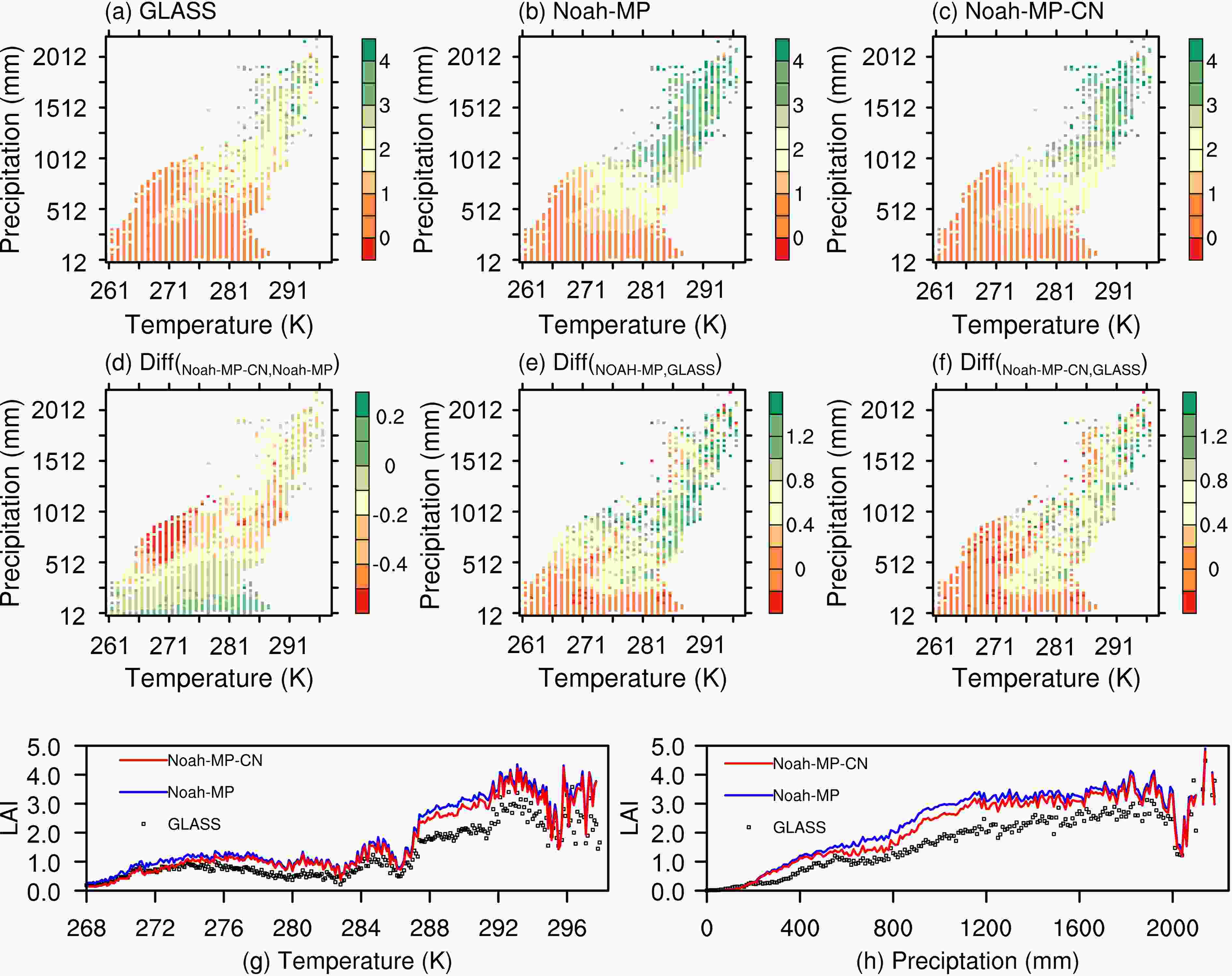
Figure 3. Distribution of multi-year averaged LAI (m2 m−2) in China relative to the variations in temperature and precipitation: (a) GLASS observation; (b) Noah-MP; (c) Noah-MP-CN; (d) Noah-MP-CN minus Noah-MP; (e) Noah-MP minus GLASS; (f) Noah-MP-CN minus GLASS. Sensitivities of LAI to (g) temperature and (h) precipitation.
We further evaluate the performances of Noah-MP-CN for cropland, forest, grassland, savanna, and shrubland, which are five major land-cover types in the study domain by comparing regionally averaged LAI values. After introducing nitrogen dynamics, all simulations are more consistent with observations than the original Noah-MP. As shown in Table 3, the RMSEs/biases of all five types are reduced, with the values ranging from 0.04/0.10 (forest) to 0.23/0.26 (cropland). Four of the five types also present better correlations, except for forest.
LAI (units: m2 m−2) GPP (units: gC m-2 d−1) Noah-MP Noah-MP-CN Noah-MP Noah-MP-CN R Bias RMSE R Bias RMSE R Bias RMSE R Bias RMSE Cropland 0.93 0.83 0.88 0.94 0.57 0.65 0.97 3.01 3.33 0.98 2.5 2.95 Forest 0.84 0.50 0.87 0.83 0.39 0.83 0.95 1.32 1.51 0.95 0.98 1.23 Grassland 0.65 0.66 0.87 0.67 0.47 0.67 0.85 0.33 0.77 0.88 0.04 0.57 Savannas 0.9 1.14 1.23 0.92 0.98 1.07 0.98 1.05 1.14 0.99 0.66 0.76 Shrublands 0.58 0.24 0.50 0.61 0.13 0.41 0.78 −0.04 0.57 0.8 −0.18 0.57 Table 3. Correlation coefficients (R), bias, and root-mean-square error (RMSE) between regionally averaged simulation and observation for LAI and GPP of different land-use types in China.
-
As the gross amount of dry organic matter, GPP is not only the key regulator for the whole ecosystem but also the main factor for the carbon sink of terrestrial ecosystems. Noah-MP overestimates multi-year mean GPP in eastern China, whereas the overestimation is reduced to some extent by Noah-MP-CN, especially in cropland regions (Fig. 4), which is also shown in Table 3 in the comparison of regionally averaged values. Future investigations on the parameters of simulated biomass-related variables are desirable to resolve the negative GPP bias and positive LAI bias over shrubland from Noah-MP-CN. Four of the five types also present better biases, except for shrublands, whose GPP is already underestimated in the default Noah-MP with the dynamic vegetation option; the nitrogen limitation in Noah-MP-CN worsens the GPP simulations in terms of bias.
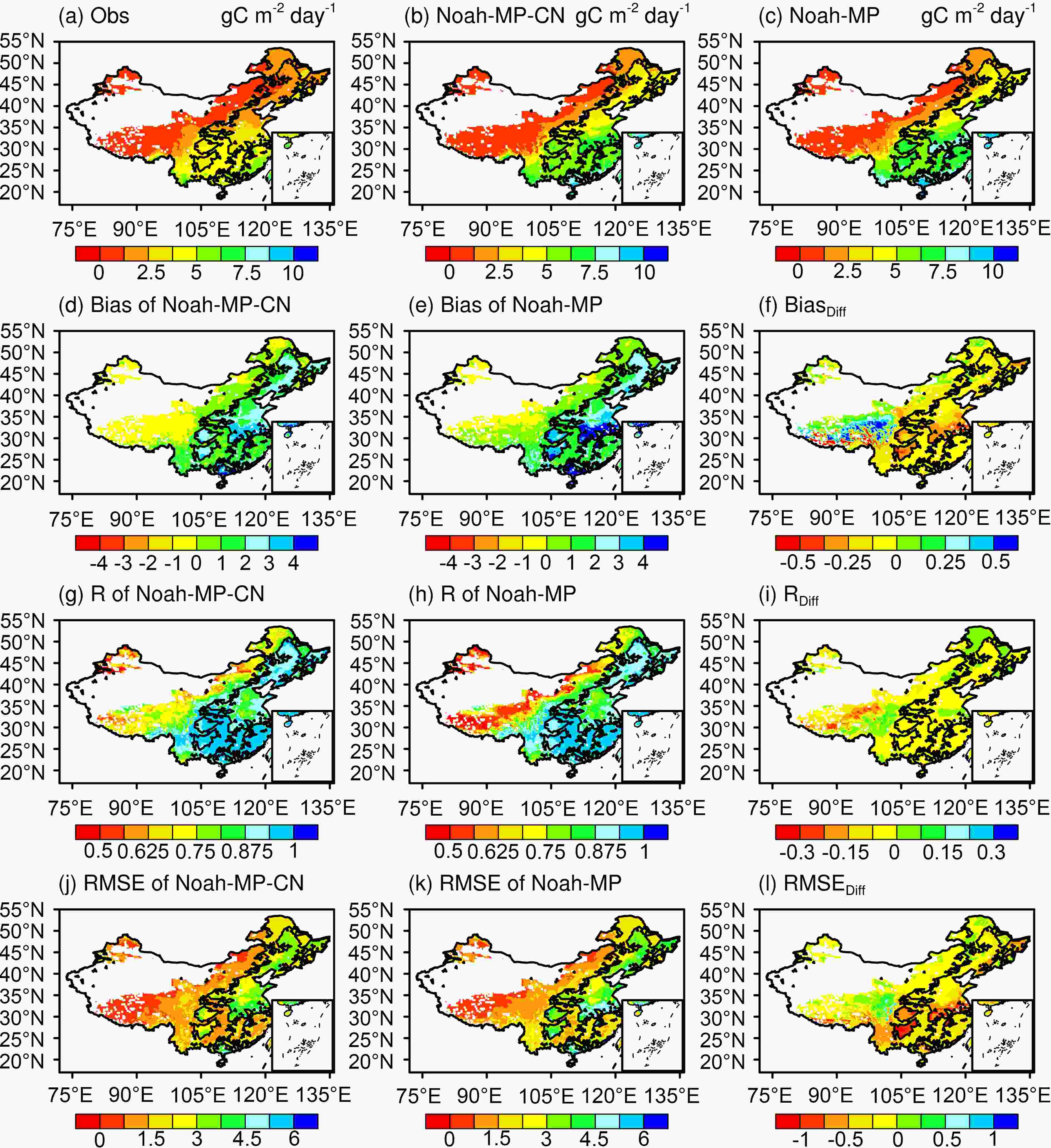
Figure 4. As in Fig. 2 except for GPP.
Despite the above-mentioned issues, Noah-MP-CN does improve the correlation in most regions, when both simulations exhibit relatively high correlation values. Additionally, reduced RMSE values are found in almost the whole domain, especially in cropland regions, which shows promise for using Noah-MP-CN in regional simulations.
-
As one of the most important land-cover types, cropland directly influences the terrestrial nitrogen cycle by accepting almost half of the total nitrogen input to the soil through fertilizer application (Fowler et al., 2013). Here, we consider three aspects directly related to coupling nitrogen dynamics for cropland: the carbon cycle, water cycle, and fertilizer application amount.
-
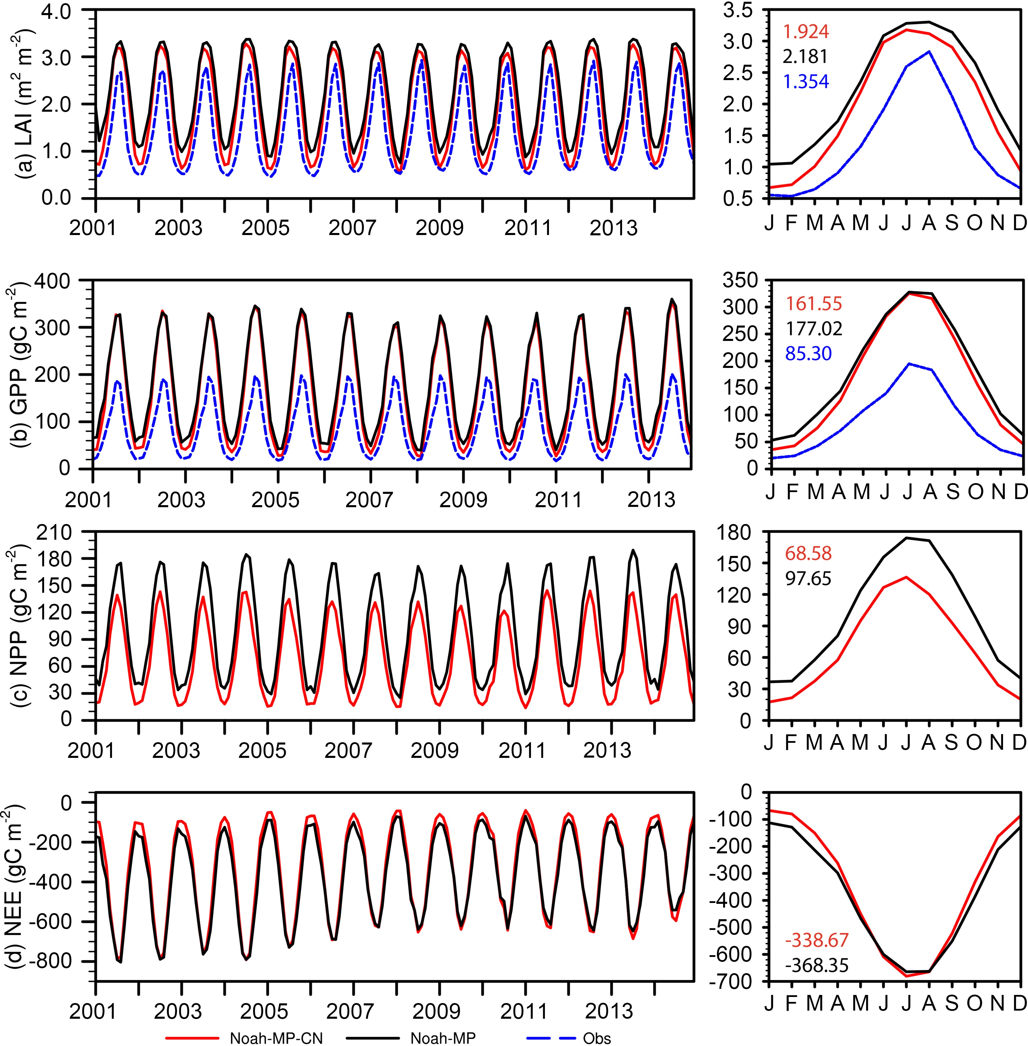
Figure 5a compares the LAI time series from Noah-MP, Noah-MP-CN, and the validation data. Both Noah-MP-CN and Noah-MP capture the variations of LAI. When coupled with nitrogen dynamics, the simulation is closer to the observation, with a 0.01 increase in R and 0.23 decrease in RMSE for the whole period (Table 3). Noah-MP-CN brings the most obvious decrease in LAI in winter, suggesting a tighter constraint of nitrogen on carbon due to the low temperature in winter.

Figure 5. Comparison of Noah-MP, Noah-MP-CN and observation on cropland for (a) LAI, (b) GPP, (c) NPP and (d) NEE, noting that observations only exist in the comparison of (a) LAI and (b) GPP. The right-hand column shows the corresponding multi-year mean seasonal cycle and the average of a month.
Figure 5b compares the monthly GPP variations from Noah-MP and Noah-MP-CN. Both models capture the slightly increasing trend of GPP during 2001−13. Specifically, Noah-MP-CN shows a similar variation to Noah-MP both in terms of trends and amplitudes, with the same R and 11.49 gC m−2 decrease in RMSE. Noah-MP-CN slightly decreases the GPP estimates from 177.02 to 161.55 gC m−2, with the largest difference occurring in winter, as directly influenced by the variation of LAI.
Figure 5c shows that Noah-MP-CN brings a large decrease in NPP (from 97.65 to 68.58 gC m−2), which means less carbon could be used by the plant, and directly results in a decrease in LAI (from 2.181 to 1.924 m2 m−2). The smaller decrease in LAI than NPP can possibly be explained by the decreased leaf turnover in the model, i.e., leaves senesce and fall, which is down-regulated by the limitation of nitrogen, reducing the amount of leaf biomass to loss. As for net ecosystem exchange (NEE), the annual mean is reduced by 29.68 gC m−2 (from 368.35 to 338.67), meaning that the carbon sink is decreased when taking the impact of nitrogen into consideration.
-
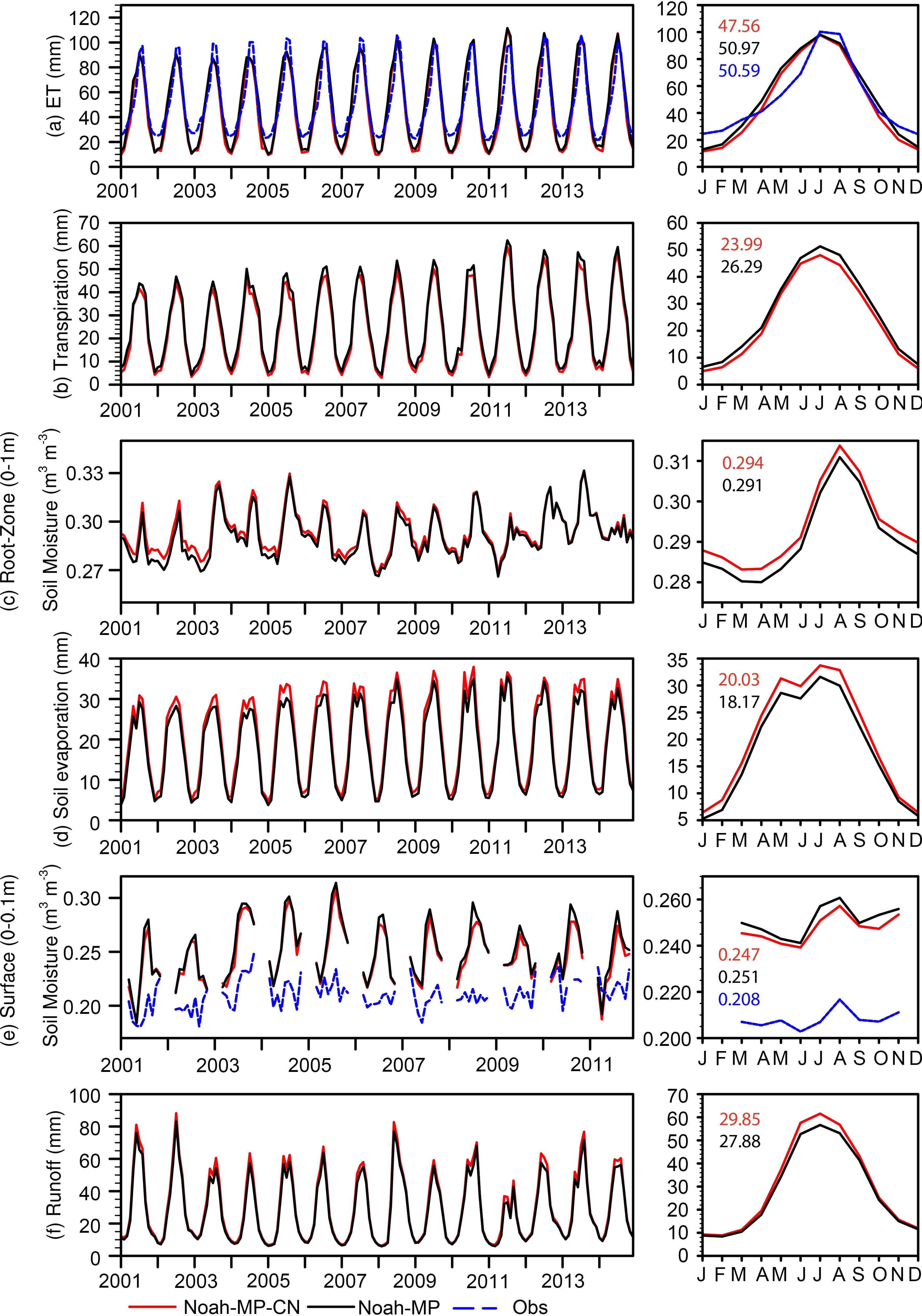
As shown in Fig. 6a, both Noah-MP-CN and Noah-MP capture the temporal variation of ET well. The differences between Noah-MP and Noah-MP-CN are insignificant. Noah-MP-CN slightly outperforms Noah-MP insofar as it produces smaller RMSE values and better temporal correlation (Table 4), despite the larger bias. The improvement is mainly attributable to the reduction in ET peaks, which is caused by the smaller LAI.
R RMSE Bias Noah-MP Noah-MP-CN Noah-MP Noah-MP-CN Noah-MP Noah-MP-CN ET (mm month−1) 0.93 0.95 14.84 14.65 0.38 −3.03 Soil moisture(mm month−1) 0.41 0.43 0.047 0.043 0.043 0.039 Table 4. Correlation coefficients (R), and root-mean-square error (RMSE), and bias between regionally averaged simulation and observation for ET and soil moisture of cropland in China.
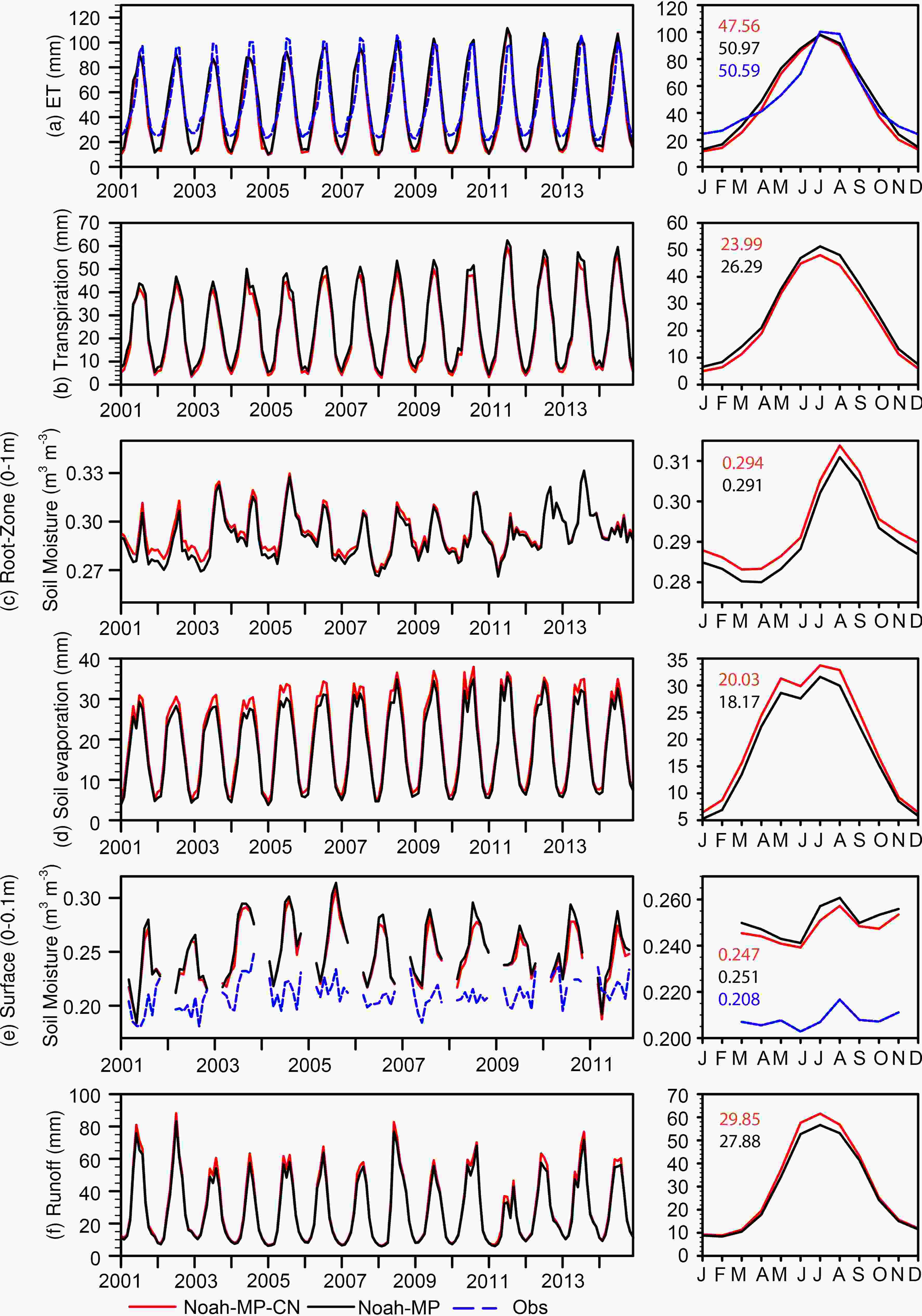
Figure 6. As in Fig. 5 except for (a) ET, (b) transpiration, (c) root-zone soil moisture, (d) soil evaporation, (e) surface soil moisture, and (f) runoff, noting that observations only exist in the comparison of (a) ET and (e) surface soil moisture.
Figures 6b-d show the impacts of nitrogen dynamics on transpiration, root-zone (0−1 m) soil moisture and soil evaporation at different time scales. Noah-MP-CN differs from Noah-MP in partitioning total ET between transpiration and soil evaporation. Note, however, that the decrease in LAI contributes directly to the decrease in transpiration, resulting in a monthly reduction of 2.3 mm, subsequently leading to more simulated root-zone (0−1 m) soil moisture (from 0.291 to 0.294) than in the original model. The decrease in LAI also leads to more exposure of the land surface, which directly increases the amount of soil evaporation (from 18.17 to 20.03 mm), subsequently reducing the surface (0−0.1 m) moisture (from 0.251 to 0.247).
Figure 6e also shows that both Noah-MP-CN and Noah-MP reproduce the variation in surface soil moisture to some extent, although the evaluation data were derived from relatively few stations (14 sites). Noah-MP-CN slightly outperforms Noah-MP in terms of a higher temporal correlation (0.43 versus 0.41) and a slightly smaller bias (0.039 versus 0.043) and RMSE (0.043 versus 0.047), as shown in Table 4.
The most notable discrepancies of Figs. 6b and d mainly occur in summer, with the contribution provided by the relatively high temperature. With the decrease in ET and soil moisture, runoff (shown in Fig. 6f) shows an increase, from 27.88 to 29.85 mm, especially during summer.
Overall, Noah-MP-CN only shows slight improvements from Noah-MP in water-related variables, as compared to carbon-related variables, which is reasonable considering the impact of nitrogen on the water cycle occurs mainly via indirect effects. Nonetheless, the slight improvement in simulating the water cycle is promising for incorporating nitrogen dynamics to improve the performances of LSMs.
-
The coupled Noah-MP-CN describes fertilizer inputs and their connections to carbon/water cycles through physical parameterizations, and thus it allows us to investigate the utilization efficiency and environmental benefit of fertilizer application.
-
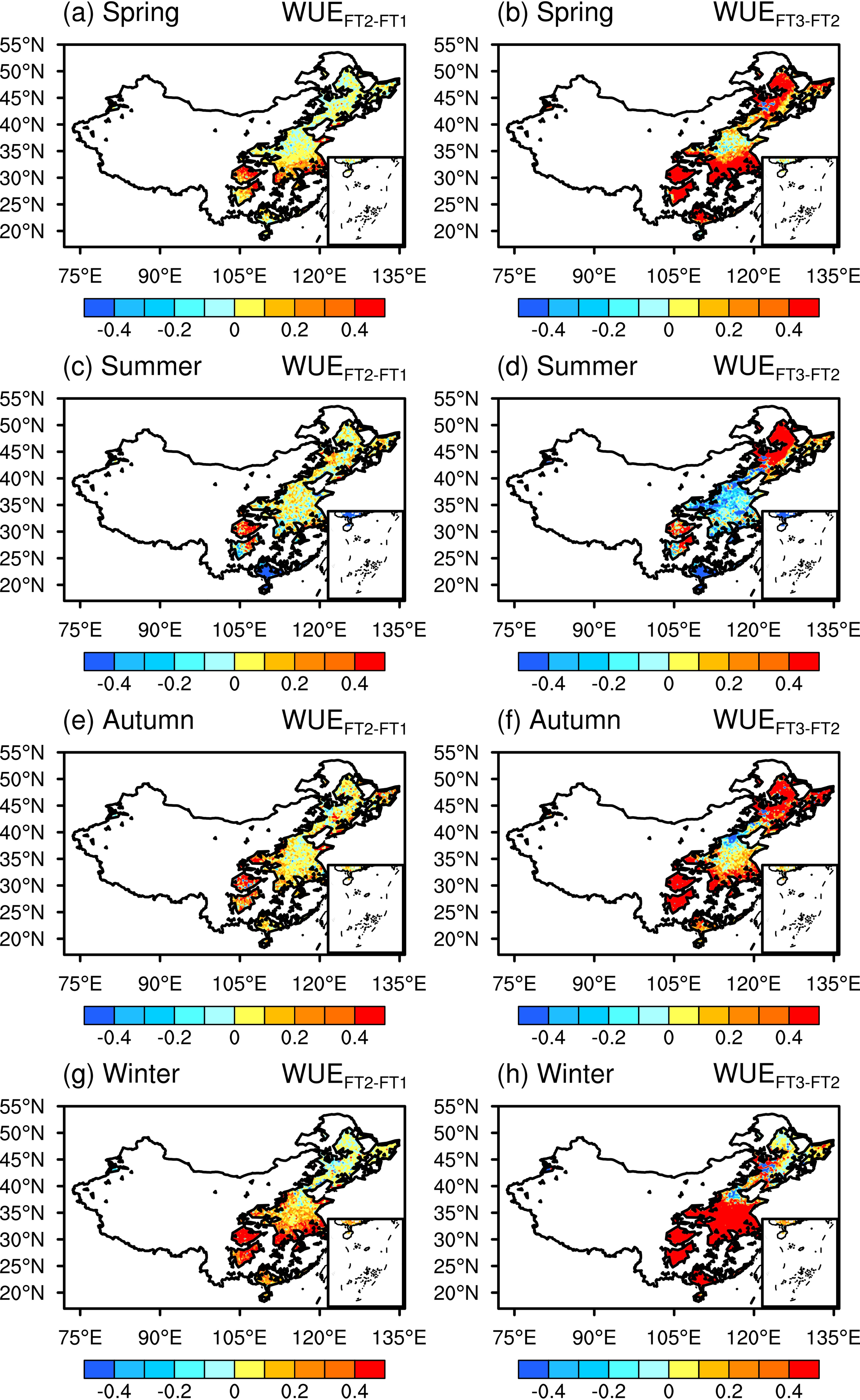
To examine the impact of fertilizer application, we use water-use efficiency (WUE) as a metric to reflect the impact of the environment on plant growth. WUE is defined as the carbon gain at the cost of unit water loss, and here we use the ratio of GPP to transpiration to define WUE.
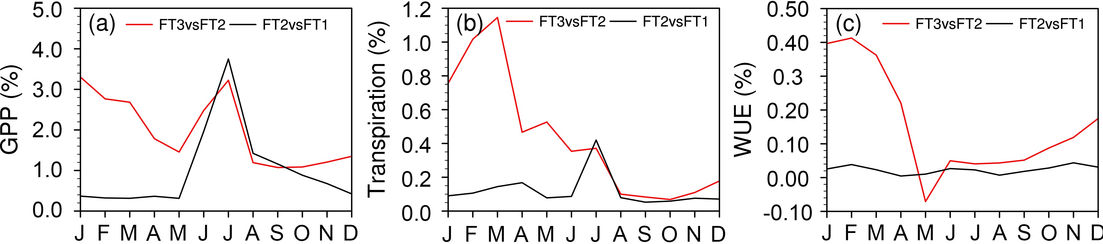
Based on the difference of the WUE spatial distribution in the seasonal cycle (Fig. 7), we find that using nitrogen fertilizer can generally increase WUE in most regions throughout the whole year, especially in winter because nitrogen fertilizer can play an important role in supporting crop growth during this season. WUE is also higher by applying the actual amount in spring, autumn, and winter, compared to applying only half the amount of fertilizer. Interestingly, although there is a general increase in WUE in most regions in FT2 compared to FT1 (Fig. 7), in summer, FT3 exhibits the lower WUE compared to FT2 in most cropland areas. Figure 8 further shows that, with an increasing amount of fertilizer, both GPP and transpiration increase in all months. GPP shows a decreasing trend before May, while obvious increasing trends for both GPP and transpiration are seen after June in FT2 versus FT1 (when fertilizer is applied), indicating this amount of fertilizer supplements the consumption of nitrogen used by cropland in the period before June to improve WUE. However, the increasing rate of WUE in FT3 versus FT2 exhibits a steep drop starting in February, which even reaches negative values in May, indicating that this amount of fertilizer may be beyond the nitrogen demands of cropland in this period, the beginning of the growing season. After some consumption of fertilizer, along with more fertilizer needed in the summer, the increasing rate of WUE returns to positive but still keeps a relatively slight growth. In other words, this high level of fertilizer application might be too much to maintain a high WUE. After the peak nitrogen consumption in summer, the surplus nitrate ensures a large increase in WUE in the following seasons, causing it to peak in spring. Numerically, compared to the halved fertilizer use, the actual fertilizer use increases GPP by only 1.97% at the cost of near-zero (0.43%) water consumption elevation for the whole cropland area.
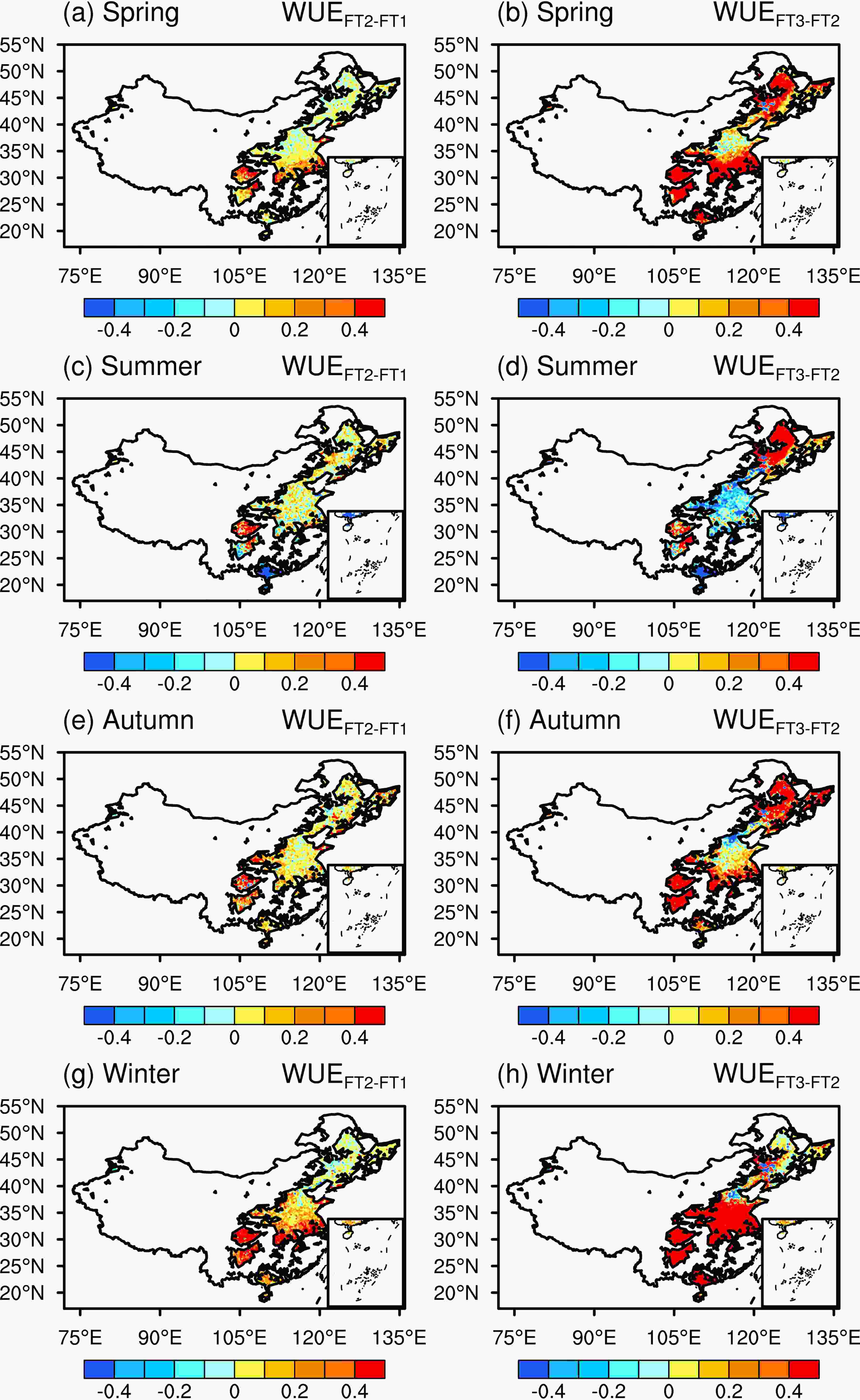
Figure 7. Differences in multi-year (2001−14) mean WUE (units: g kg−1) between FT1 and FT2 (left-hand column) and between FT2 and FT3 (right-hand column) for spring, summer, autumn, and winter.
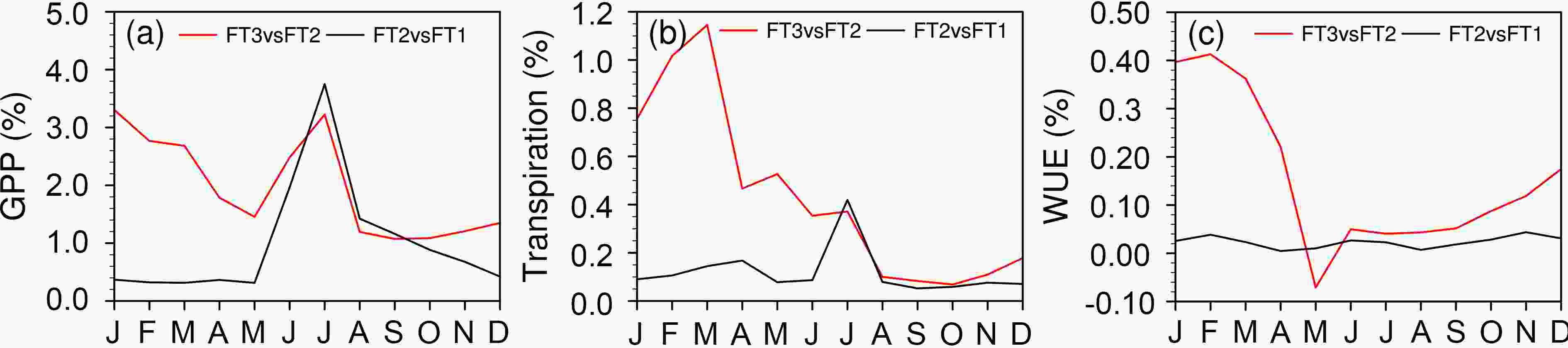
Figure 8. Mean seasonal cycle of percentage change for (a) GPP, (b) transpiration, and (c) WUE between FT1 and FT2 and between FT2 and FT3 in cropland during 2001−14.
Overall, our modeling results suggest that appropriate fertilizer use can increase the grain yield and WUE, while excessive use will reduce WUE, which means a waste of resources. Only when we apply fertilizer properly (in terms of amount), can we make the best of it. These modeling results clearly demonstrate such effects by scrutinizing the nitrogen dynamics in cropland regions of China, demonstrating the model’s suitability for a range of future applications involving agricultural decision-making.
-
Leaching, as the main indicator of water pollution, is chosen as an indicator to further investigate the impacts of nitrogen fertilizer application on the environment. The combination of the nitrate transported to rivers via surface and subsurface runoff, and to groundwater through percolation from the soil bottom, is used as the total amount of nitrate leaching in this study.
All three experiments share a similar spatial pattern of annual leaching, and the overall magnitudes of FT3 are reasonable (Fig. 9), which is consistent with previous studies (Manevski et al., 2016). High values are seen in northern China, especially in the croplands of the Loess Plateau, Huang-Huai-Hai Plain, and Songliao Basin, where relatively high amounts of fertilizer have been applied. These regions also show an obvious increase in nitrogen leaching between different amounts of fertilizer. The increase in the amount of leaching of FT3 relative to FT2 (5.35%, based on FT2) is almost twice that of FT2 to FT1 (5.91%, based on FT1), indicating a strong contribution of fertilization application to leaching when it reaches a certain threshold. These results point to the potential of Noah-MP-CN as a tool in managing cropland fertilizer use to enhance productivity while minimizing pollution.

Figure 9. Multi-year mean nitrate leaching during 2001−14 for cropland in China: (a) FT1 leaching; (b) FT2 leaching; (c) FT3 leaching; and the increase percentage between (d) FT1 and FT2, (e) FT2 and FT3, and (f) FT1 and FT3.
4.1. Regional model performance over China
4.1.1. LAI
4.1.2. GPP
4.2. Cropland
4.2.1. LAI, GPP, NPP, and NEE
4.2.2. ET, runoff and soil moisture
4.3. Sensitivities to fertilizer application amount
4.3.1. Water-use efficiency
4.3.2. Nitrogen leaching
-
This study represents the first regional application of Noah-MP-CN over a complex domain such as China. Noah-MP-CN incorporates the plant nitrogen uptake from FUN and the soil nitrogen dynamics from SWAT. On the basis of previous point-scale work by Cai et al. (2016), we developed a regional-applicable version by explicitly accounting for spatially varying biogeochemical parameters. A series of simulations were then conducted over China using the newly developed Noah-MP-CN and original Noah-MP. The two models are compared in modeling the terrestrial carbon and water cycles and evaluated against observations.
Overall, it was found that Noah-MP-CN simulates the carbon and water variables over China reasonably well. The evaluation showed that incorporating nitrogen dynamics improves the simulations of GPP and LAI in most regions in terms of a slightly higher correlation coefficient, a much lower RMSE, and a better spatial pattern of multi-year climatologies. The overestimation of GPP by Noah-MP with a dynamic vegetation option is greatly improved by considering the limitation of nitrogen availability, especially in southeastern regions of China. Moreover, Noah-MP-CN provides a more accurate LAI simulation in different land-cover types, with reduced RMSEs and increased correlations. Compared to Noah-MP, Noah-MP-CN provides more reasonable variations of LAI along with different precipitation and temperature. The improvement in simulating LAI is demonstrated in most regions, but especially in the humid warm regions, with temperatures exceeding 8°C and precipitation of more than 800 mm.
Fertilizer application on croplands accounts for half of the total nitrogen input to soil (Fowler et al., 2013). The increased nitrogen availability affects both the carbon cycle and the water cycle in this study. Overall, it was found that the simulated LAI, GPP, ET and soil moisture show higher correlation coefficients and much smaller RMSEs, especially for LAI. The impacts of fertilizer application on plant WUE and nitrogen leaching into the environment were further examined, revealing that the simulated seasonal dynamics of WUE and leaching are physically reasonable. Compared to the halved fertilizer use, the model indicates that the actual amount of fertilizer use increases GPP by only 1.97% at the cost of a near-zero (0.43%) elevation of water consumption and a 5.35% increase in nitrogen leaching. These results suggest that the amount of fertilizer applied in recent years may have been excessive, which is consistent with previous studies (Ren et al., 2012). In other words, the current level of fertilizer use has only a negligible impact on water consumption but a damaging impact on the environment. Due to a lack of direct observations, this finding still needs to be further confirmed, but our study is nevertheless the first to pin down these numbers at the regional scale using a carefully developed and evaluated model. It suggests that a broader investigation of the economic and environmental implications is warranted in the future.
This study shows that Noah-MP-CN outperforms Noah-MP. However, it remains a challenging question as to what processes lead to the improvements. First, there are complex interplays among the nitrogen, carbon, and water processes. The augmented Noah-MP-CN considers the dynamic constraints of nitrogen on photosynthesis, while the carbon assimilated by photosynthesis is spent to take up nitrogen from soils. The plant nitrogen uptake is modulated by soil nitrogen availability. Photosynthesis is closely coupled with transpiration, which modulates soil moisture, which in turn influences the passive nitrogen uptake by transpiration from each soil layer. Second, there are complex interactions between processes and parameters. For example, different plant types have different demands in taking up nitrogen from the soil, while each soil texture type can determine the storage capacity of soil nitrogen and the conversion between various forms of soil nitrogen. Third, there are also complex interactions between the modules and their inputs. Precipitation can determine the nitrogen deposition into the soil. Fertilization directly changes the soil nitrogen availability. In this study, we conducted a series of sensitivity experiments with different amounts of fertilizer application. In these experiments, Noah-MP-CN behaved reasonably. In the future, more systematic sensitivity tests (Zheng et al., 2019) should be carried out to elucidate the dominant processes for different regions and seasons.
Despite the superior performance of Noah-MP-CN over Noah-MP, there is still room for improvement as Noah-MP-CN continues to overestimate LAI and GPP. This possibly suggests a systematic bias whose causes need further research. In addition, more biogeochemical processes are needed in the next steps of model development. For example, soil organic matter (SOM) dynamics has not been incorporated. SOM represents the largest global reservoir of terrestrial organic carbon, which not only can affect the storage of nutrients in the soil (especially for nitrogen) but also result in environmental pollution. Moreover, lakes and wetlands need to be implemented in the model. They are the landscape hotspots for storing carbon, burying it within sediments and releasing it into the atmosphere. These lake- and wetland-related nitrogen effluxes may potentially contribute to a significant portion of nitrogen released to the atmosphere annually, but they are not explicitly modeled here. Last but not least, considering the importance of nitrogen deposition on the carbon cycle and its great changes in recent years (Lu et al., 2012), a newly developed dynamic dataset of nitrogen deposition should be implemented to compensate for the relatively simplified parameterization in the current model. Future modeling efforts should make relevant improvements in this regard, in order to improve our understanding of the complex interactions among the components of biogeochemical cycles and their impacts on the water cycle and weather/climate.
Acknowledgements. This work was supported by the National Key Research and Development Program of China (Grant No. 2018YFA0606004) and the National Natural Science Foundation of China (Grant Nos. 91337217, 41375088, and 41605062). The first author acknowledges the support of the China Scholarships Council. Data support from “Loess Plateau Data Center, National Earth System Science Data Sharing Infrastructure, National Science & Technology Infrastructure of China (
http://loess.geodata.cn )”, is also acknowledged.Electronic supplementary material: Supplementary material is available in the online version of this article at
https://doi.org/10.1007/s00376-020-9231-6 .
 AAS Website
 AAS WeChat