Simulated Sensitivity of Ozone Generation to Precursors in Beijing during a High O₃ Episode

As one of the important sources of free radical OH in the atmosphere, ozone plays a very important role in the atmosphere (Oltmans and Levy, 1994). Ozone troposphere is an important pollution gas, and inhalation of ozone can cause respiratory diseases, affecting human health (Wang, 1999; Tang et al., 2006). The major precursors for ozone generation in the troposphere are nitrogen oxides (NO_x) and volatile organic compounds (VOCs). The VOCs are any organic solid or liquid that can volatilize at normal temperature and pressure. At present, more than 300 kinds of VOCs have been identified, including alkanes, aldehydes, aromatics and esters (Lu et al., 2006; Wang et al., 2009).

In recent years, with the improvement of fine particulate pollution control in China, the problem of ozone pollution has become increasingly paramount (Zhang et al., 2015; Wang et al., 2017). In order to better control ozone pollution, two key scientific questions need to be addressed. One is that ozone can exist for a long time in the atmosphere, being able to travel a long distance and forming regional pollution. So, to control ozone pollution, it is necessary to analyze the relative contributions of ozone local generation and regional transportation, and, at the same time, to implement regional joint prevention and control. Another problem is that the chemical mechanism of ozone generation is complex, and the relationship between ozone and its precursors (NO_x and VOCs) is nonlinear, so the sensitivity of ozone to its precursors should be diagnosed to find the optimal ratio of precursor NO_x/VOC_S reduction (Wu et al., 2017). The sensitivity of ozone to its precursors can be partitioned into NO_x sensitivity, transition sensitivity, and VOC sensitivity. In an NO_x sensitive area, with the reduction of NO_x emission, O₃ decreases faster than VOCs, while in the sensitive area of VOCs, the reduction of NO_x emission may lead to an the increase in O₃ (Guicherit and van Dop, 1977), whereas somewhere between the two is the transition sensitivity.

As the capital of China, Beijing has performed considerable work in environmental protection, and much research has been conducted on the sensitivity of Beijing ozone to its precursors. Xu and Zhang (2006) used the CMAQ model to simulate the summer O₃ in Beijing and found that the O₃ generation in Beijing was VOCs-limited. An (2007) pointed out that the Beijing O₃ concentration is mainly controlled by VOCs. Tang et al. (2010) indicated that the current ozone formation in Beijing is under NO_x-saturated conditions. Lu et al. (2010) adopted the OBM model to study the rate of O₃ photochemical production and its controlling factors in Beijing, which indicated that the chemical production of O₃ in Beijing is controlled alternately by VOCs and NO_x. The changes in controlling factors are closely related to the activity of VOCs and the concentration of NO_x. Nie et al. (2014) used CMAQ to simulate the ozone precursor control area in Beijing and showed that the contribution from the Huairou Distinct in the NO_x control area is the highest in summer. Gao et al. (2016) used the multi-scale meteorological air quality model (MCCM), and found that ozone in the Beijing-Tianjin-Hebei region was controlled by both NO_x and VOCs. Although the VOCs reduction was the main contributor, the NO_x reduction was also considered.

The EKMA curve method (empirical kinetic simulation method) is a classical method to study the sensitivity of ozone to its precursors. The EKMA curve can reflect the VOC_S- NO_x-O₃ relationship. In 1977, American scientist Dodge obtained the EKMA curve using the ozone concentration curve model OZIPP (Ozone Isopleth Plotting Package) under certain assumptions (Dodge, 1977). Calculate the daily maximum ozone concentration and draw the ozone peak concentration isoline through precursors (NO_x and VOCs) with different initial concentrations in the absence of any photochemical reaction (Tan, 2015). The ozone concentration and the emission source of precursors are nonlinear, which is not suitable for the atmospheric diffusion model of total load distribution, but the EKMA method solves this problem well (Tang et al., 2006). By transforming the problem of ozone control into the control of primary pollutants NO_x and VOCs, the reduction scheme needed to control precursors can be given quantitatively. Subsequently, others improved the classical EKMA curve drawing method and studied the sensitivity of ozone precursors by combining model calculation with the EKMA curve. Altshuler et al. (1995) analyzed the relationship between the weekend effect and ozone precursor sensitivity in 1980−1990 by using EKMA and an air pollution model. Li et al. (2017) found that ozone in Langfang was a VOCs-controlled area by combining EKMA and the VOCs/NO_x ratio. Zhou et al. (2014) used the MM5 and CMAQ models to simulate the O₃ generation in Tianjin. They found that Tianjin lies in the VOC control area. In summer, more than 40% of VOCs should be reduced to avoid the further increase of O₃. Bei et al. (2017) used the WRF-Chem model and found that Xi'an belongs to an NO_x-limited area. Shen et al. (2018) found that ozone was controlled by VOCs in the Pearl River Delta region by combining the WRF model with EKMA.

In this paper, the WRF-Chem model is utilized together with the EKMA method to analyze the complex pollution process in Beijing during 13−23 May 2017. By setting the sensitivity tests and the EKMA curve, the sensitivity of ozone to its precursors in Beijing was studied, and the emission reduction scheme was formulated.

This paper uses the hourly O₃, NO₂, PM_2.5 and PM₁₀ mass concentration observation data from 13 to 23 May 2017. The observation data used for the model test are the hourly data from the automatic monitoring network of Beijing Environmental Protection Monitoring Center (http://zx.bjmemc.com.cn). At present, the Beijing Municipal Environmental Protection Bureau has established 35 atmospheric environmental quality monitoring stations in Beijing. In this study, three monitoring stations, including Changping (40.22°N, 116.22°E) and Shunyi (40.18°N, 116.66°E) Stations in the suburbs and Wanshou West Palace (39.89°N, 116.36°E) Station in an urban area, are selected for monitoring data analysis (Fig. 1).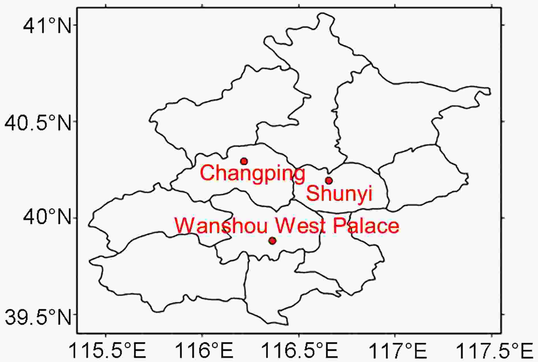

Figure 1.  Locations of Changping Station (40.22°N, 116.22°E), Shunyi Station (40.18°N, 116.66°E) and Wanshou West Palace Station (39.89°N, 116.36°E) in Beijing. (Changping and Shunyi Stations are in the suburbs and Wanshou West Palace Station is in an urban area)

The O₃ analyzer uses Thermo Fisher 49i ultraviolet spectrophotometry analyzer, and the NO_x analyzer uses Thermo Fisher 42i chemiluminescence NO-NO₂- NO_x analyzer. The PM_2.5 and PM₁₀ monitors use Thermo Fisher Micro Oscillation Balance (TEOM) Environmental Particulate Monitor (Wang et al., 2014; Zhai et al., 2019). All observation data are calibrated and controlled in accordance with the Chinese environmental protection standard HJ 618−2011 to ensure the accuracy and validity of the monitoring data.

WRF-Chem (Weather Research and Forecasting model coupled with chemistry) is a fully coupled chemical transport model developed by NOAA and NCAR. The Institute of Earth Environment, Chinese Academy of Sciences further optimized it, having made it more suitable for air pollution simulation in China (Li and Feng, 2016).

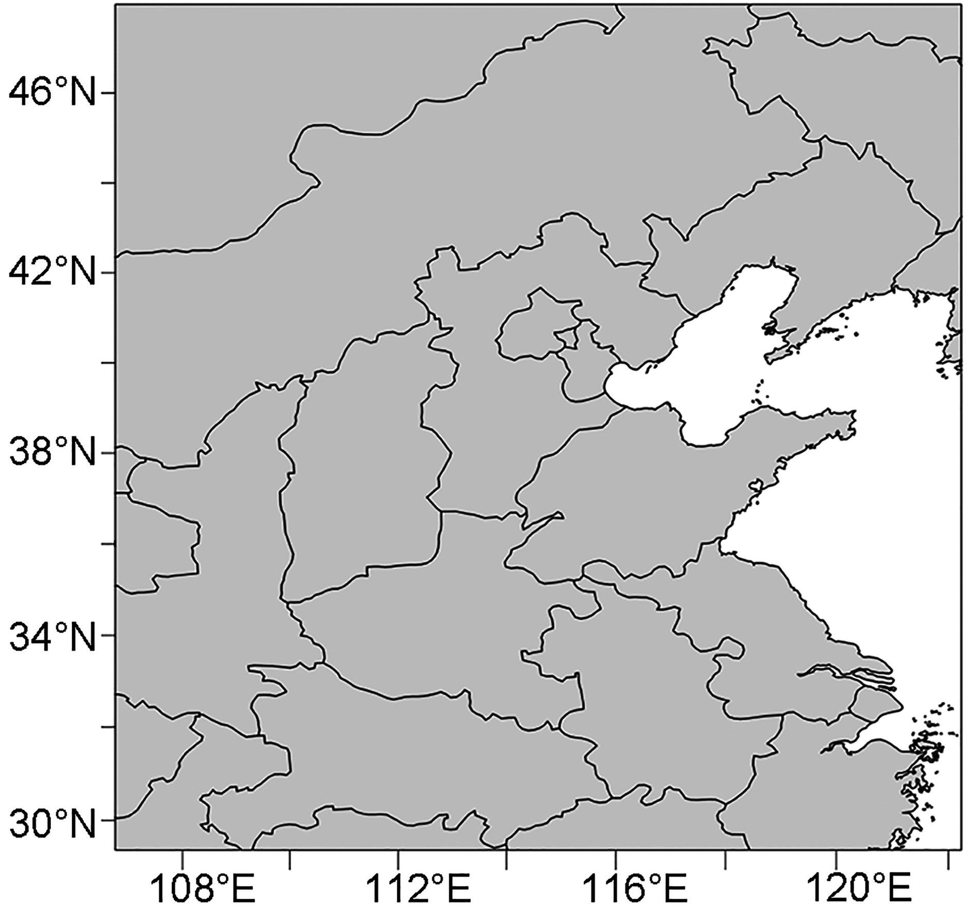
The simulation period in this paper is from 2000 LST (LST = UTC + 8) 13 May to 2000 LST 23 May 2017, and the first three days are the spin-up time. The simulation center point is at (38°N, 116°E), and the Lambert projection is adopted. The simulation domain is concentrated in North China, which is shown in Fig. 2, composed of 300×300 grid points with a horizontal resolution of 6 km, 32 layers in the vertical direction, and a simulation time step of 30 s. The initial meteorological field and boundary conditions use NCEP FNL 1°× 1° data. The chemical field uses the data output by the MOZART global chemical model every 6 hours. The emission list is provided by Tsinghua University, and the chemical mechanism adopts SAPRC99. The emission list of biological emission sources adopts the online MEGAN (Model of Emissions of Gases and Aerosols from Nature) (Guenther et al., 2006).

Figure 2.  The model simulated area.

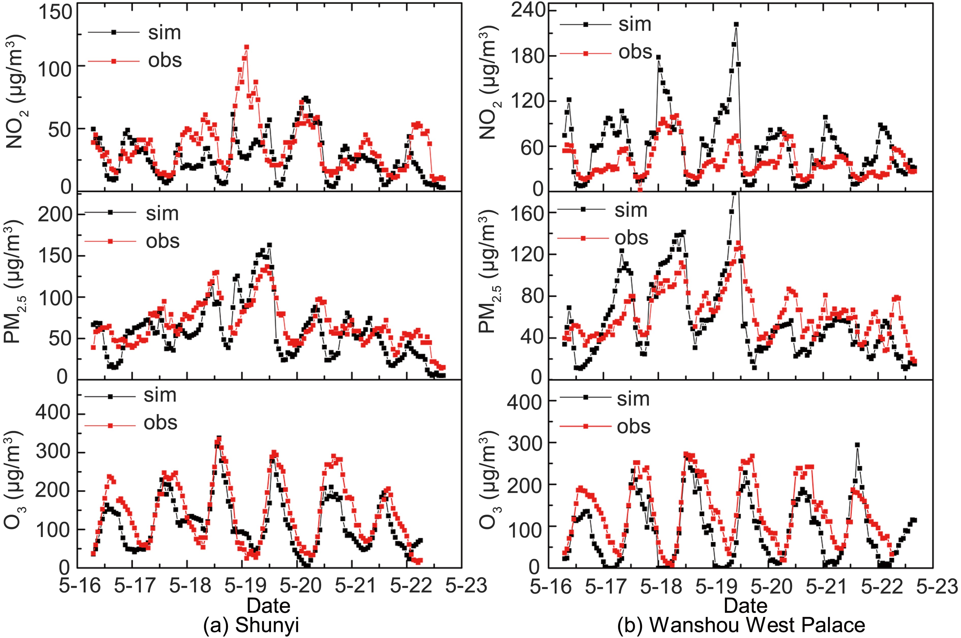
Figure 3 shows the variation curves of O₃, PM_2.5 and NO₂ concentrations and scatter plots from the model simulation and observations at Shunyi Station and Wanshou West Palace Station in Beijing during 16−22 May, 2017. Table 1 shows the MB (Mean Bias), NMB (Normalized Mean Bias), RMSE (Root Mean Square Error) and R (Correlation Coefficient) of simulated and observed O₃, PM_2.5 and NO₂ at the Shunyi and Wanshou West Palace Stations. It can be seen that both the MB and NMB indicators of O₃ are low. The simulated values for Shunyi and Wanshou West Palace are 28.52 µg m^–3 and 43.38 µg m^–3 lower than the observations, respectively. RMSE indicates that the difference between the simulated average concentration and the observed average fluctuates greatly, but the correlation coefficients of O₃ at the two sites are above 0.8, showing well the daily trend of O₃ concentration. For PM_2.5, we can see from the MB, NMB and RMSE indicators that the simulated value is lower than the observed value, but the difference between the simulated value and the observed value is not large, with the correlation coefficient being higher than 0.7. Simon et al. (2012) suggested that the reduction of nitrate, sulfate and OC concentrations is one of the reasons for the underestimation of PM_2.5 in summer. NO₂ and O₃ are significantly negatively correlated, and the NO₂ simulation effect is not as good as those for O₃ and PM_2.5. The suburban correlation coefficient is 0.48 and urban area correlation coefficient is 0.64. The simulated value of NO₂ at Shunyi Station is lower than the actual value, while the simulated value of NO₂ at Wanshou West Palace Station is higher than the observation.

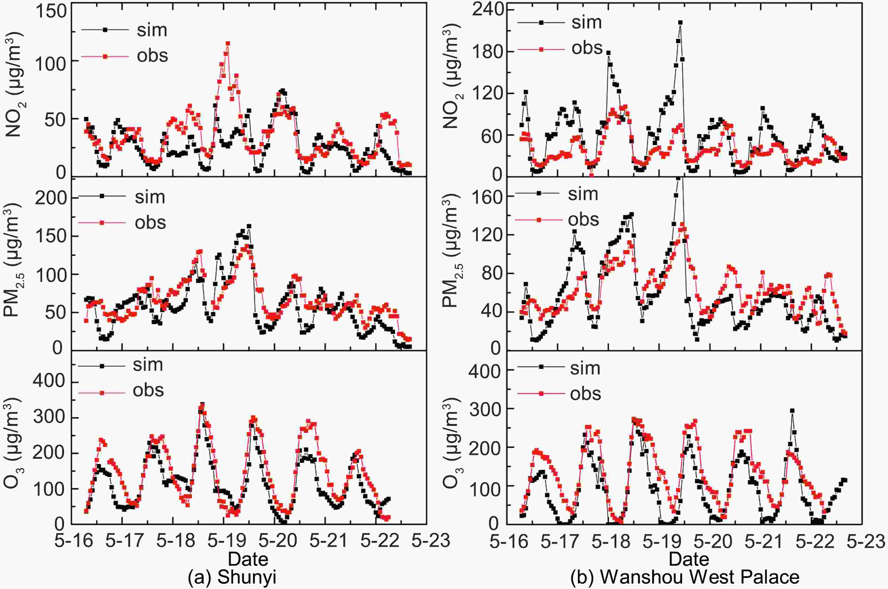
Figure 3.  Variation curves and scatter point fittings of the observed and simulated O₃, PM_2.5 and NO₂ hourly concentrations at (a) Shunyi Station and (b) Wanshou West Palace Station from 16 to 22 May 2017.

Although the simulated values are lower than the observed values as a whole, the WRF-Chem model can accurately reflect the daily variation trends of O₃, PM_2.5 and NO₂ concentrations. MB, NMB, RMSE and R have low error levels, and their resulting errors are within the acceptable ranges. The WRF-Chem model is good at simulating the photochemical pollution and haze pollution process of the composite continuous pollution, and also is able to simulate the evolution of the pollution process and the spatiotemporal distribution of pollutants. The simulation results can better reflect the change characteristics of pollutants and can provide a reference for Beijing's air quality potential forecast.

The EKMA (Empirical Kinetic Modeling Approach) curve method is a classical method to study the sensitivity of ozone to its precursors, which was obtained by American scientist Dodge in 1977 using the ozone isopleth plotting package under assumptions (Dodge, 1977; Ou et al., 2016). EKMA curve solves the problem of nonlinearity between ozone and its precursors (NO_x and VOCs), which not only has a qualitative basis for ozone control but also has a quantitative effect (Zou, 2013).

As a link between primary pollutants and secondary pollutants, EKMA curve expresses the nonlinear relationship between them, namely

C represents the concentration, C(NO_x0, VOC_S0) refers to the initial concentration without photochemical reaction, and the daily maximum concentration of O₃ is calculated based on the mixture of different initial concentrations of ozone precursors. The control problem of O₃ can be transformed into the control of primary pollutants NO_x and VOC_S, and the reduction scheme needed for total amount control can be given quantitatively (Li et al., 1998).

In this paper, the sensitivity of ozone to its precursors in the complex pollution process is studied by using the WRF-Chem model combined with the classical EKMA curve drawing principle (Ou et al., 2016; Chen et al., 2019). By inputting meteorological fields, biological sources and chemical fields (precursors with different initial concentrations) into the WRF-Chem model for photochemical reaction simulation, the daily peak concentration of ozone is obtained and the isoline of ozone peak concentration is plotted.

The specific method we used consists of utilizing 0%, 25%, 50%, 75%, and 100% of the precursors (NO_x and VOCs) to distribute emission sources to form an emission reduction matrix, that is, 1 base and 24 sensitivity test schemes. Then, we utilize the peak concentrations of these 25 trials (the specific test plan settings are shown in the first 25 entries in Table 2) to plot the EKMA curve through interpolation.

Sensitivity of ozone to precursors (NO_x and VOCs) can be divided into NO_x sensitivity, VOCs sensitivity and transition sensitivity. NO_x sensitivity is that when NO_x and VOCs emissions are reduced in the same proportion, the NO_x reduction causes O₃ concentration to decrease more; when the emission of NO_x and VOCs are increased in the same proportion, the increase of NO_x causes the O₃ concentration to increase more. VOCs sensitivity is that when NO_x and VOCs emissions are reduced in the same proportion, VOCs reduction causes O₃ concentration to decrease more; when NO_x and VOCs emissions are increased in the same proportion, the increase of VOCs leads to more increase in O₃ concentration. The overly-sensitive areas are neither NO_x sensitive nor VOCs sensitive (Liang et al., 2006).

The specific test scheme settings of all the sensitivity tests in this paper are given in Table 2. All sensitivity tests are only for anthropogenic emission sources, and the emission from biological sources will not be changed. The disturbance of NO_x and VOCs emission sources is linearly distributed in time and space (Ye et al., 2016).

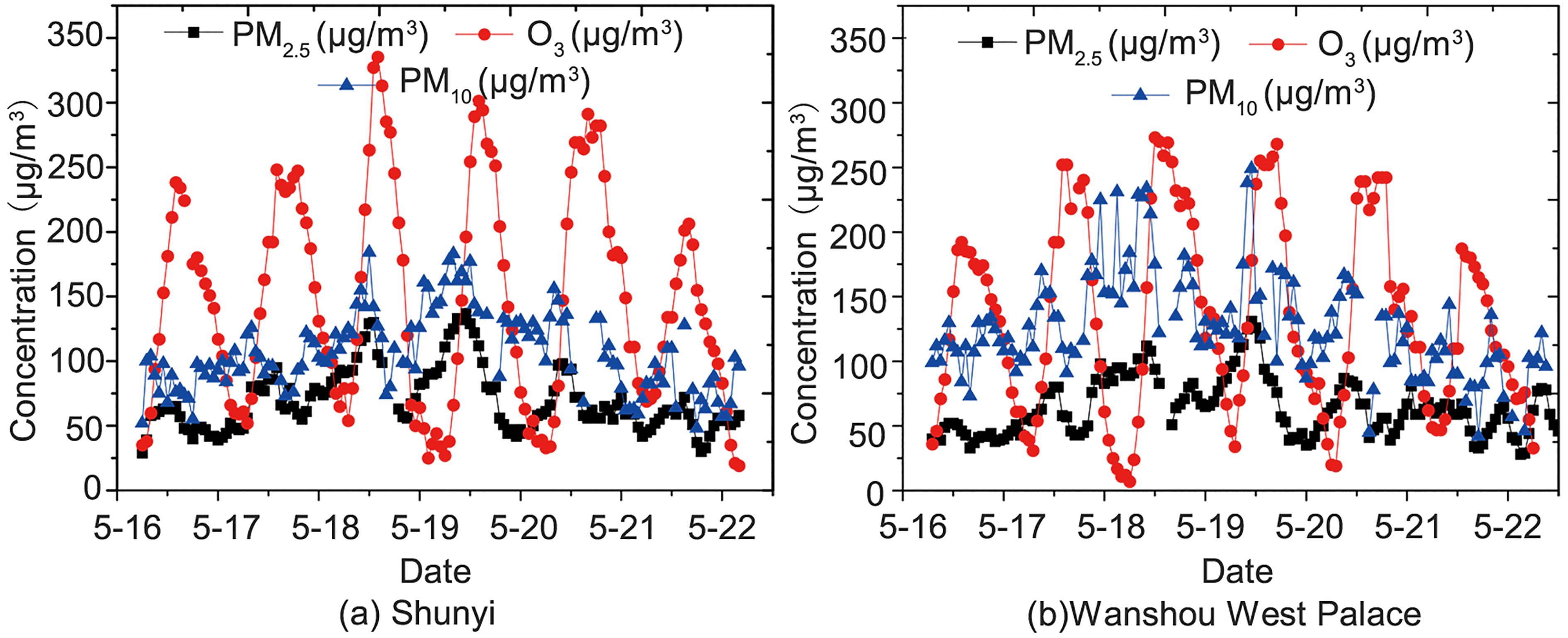
Figure 4 is a pollutant concentration chart of a mixed continuous pollution process from 16−22 May 2017. The O₃-8h (O₃-1h) average concentrations during the 16−21 May period was 183.7 µg m^–3 (146.4 µg m^–3) in Shunyi Station and 216.7 µg m^–3 (133.5 µg m^–3) at Wanshou West Palace Station. It can be seen from the figure that photochemical smog pollution and haze pollution occurred at the same time, with obvious characteristics of atmospheric composite pollution. The photochemical smog pollution in suburbs was more serious than in urban areas, and the haze pollution in urban areas was much heavier than in suburbs. The main reason for the heavier urban haze pollution is that the man-made emissions in urban areas are more than in suburbs. As for the heavier photochemical pollution in suburbs, there are two reasons: one is that urban vehicles emit NO_x with high concentrations inhibiting the production of ozone, and another is that air masses with high concentrations of NO_x are transported from urban areas to suburbs, and, meanwhile, the highly reactive VOC_S emitted by biological sources in the suburbs is added to the ozone generation reaction, thus resulting in higher photochemical pollution in the suburbs. On the 22nd, the concentration of three pollutants decreased as the result of precipitation, and the composite continuous pollution process ended.

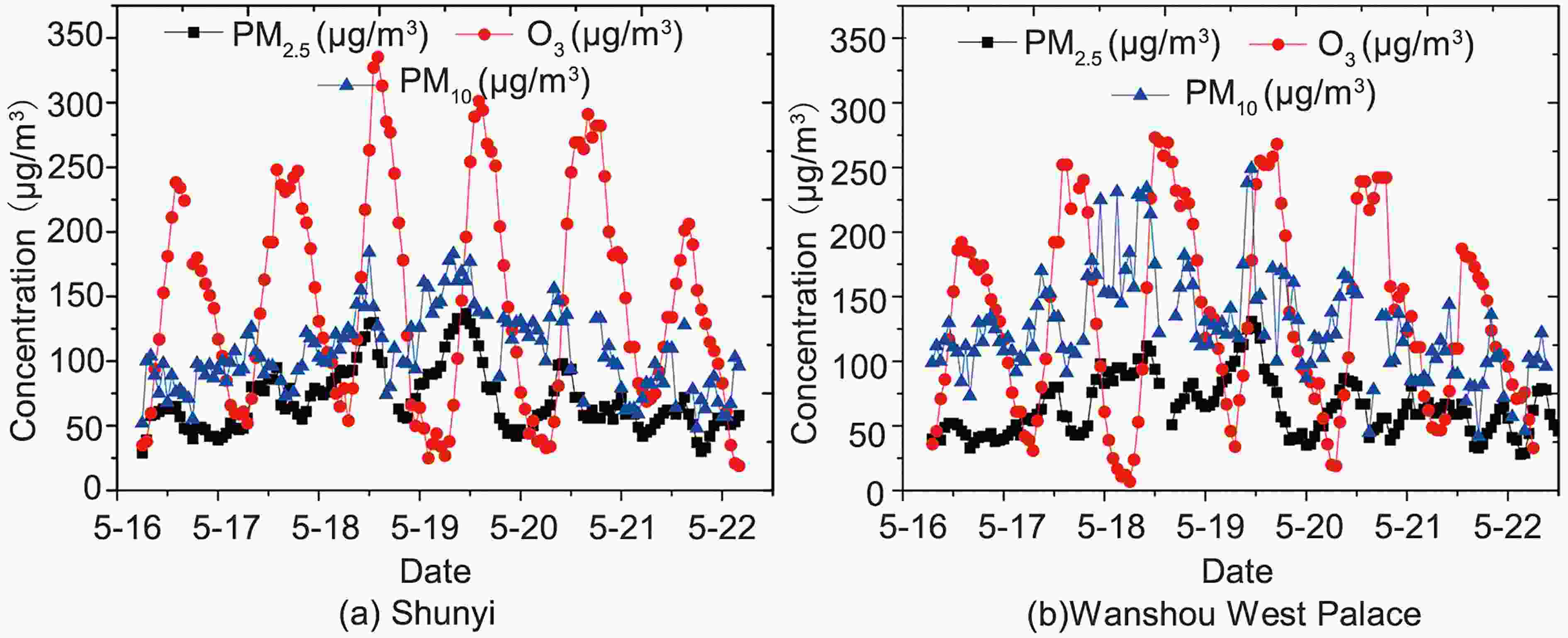
Figure 4.  Concentration of O₃, PM_2.5 and PM₁₀ pollutants at (a) Shunyi Station and (b) Wanshou West Palace Station from 16 to 22 May 2017.

From 16 to 22 May, O₃ showed a 24h periodic fluctuation. The average concentration of O₃-1h in suburbs was higher than that in urban areas. The lowest ozone concentration appeared at about 0500 LST. As the solar radiation and temperature rose, photochemical reaction became active, making the ozone concentration increase, with the peak value seen in the afternoon (1200−1600 LST). On 18 May, the pollution worsened most seriously with the maximum values of 327 µg m^–3 appearing at 1300 LST in the suburbs and 273 µg m^–3 at 1200 LST in the urban areas on 18 May, and then the values slowly went down till the next day before sunrise. During 16−22 May, PM_2.5 and PM₁₀ showed a cyclical fluctuation upward and then declined. The suburban PM_2.5 reached its peak value of 133 µg m^–3 at 0900 LST 19 May while PM₁₀ reached its maximum 184 µg m^–3 at 1200 LST 18 May. The peak values of urban PM_2.5 and PM₁₀ appeared at 1100 LST 19 May, being 131 µg m^–3 and 249 µg m^–3, respectively.

From 16 to 19 May, the weather situation in Beijing consisted of ample sunshine and high solar radiation, and the temperature continued to rise. On the 19th, the surface daily high temperature in Beijing rose to 36.8°C with lower humidity, which was conducive to the accumulation of pollutant concentration. On the 20th, a small trough fluctuation occurred, the temperature cooled and the concentration of pollutants decreased. On the 22nd, a cold front brought precipitation causing relative humidity to be 80% and dropping the daily high to 22.8°C. Such low temperature and high humidity were not helpful for pollutant accumulation, so the concentrations of the three pollutants decreased.

The high-altitude atmospheric circulation situation was characterized by Beijing being located ahead of a ridge behind the trough during the period from 16 to 19 May 2017, hence under the control of northerly airflow. The middle troposphere consisted of a warm ridge, which resulted in the temperature rise. On the 19th, Beijing's daily maximum temperature rose to 36.8°C. At 0800 LST on the 20th, the 500 hPa low vortex moved southeastward from Xi'an to Taiyuan west of Beijing, and Beijing became influenced by a southeasterly wind. From 2000 LST 20 May to 0800 LST 21 May, a small trough fluctuated at 500 hPa and, from 2000 LST 21 May to 2000 LST 22 May 2017, the trough deepened to the east and the airflow in Beijing turned to southwest before the trough.

The surface synoptic situation consisted of the high-pressure ridge over Beijing being under the influence of the post-frontal high pressure from 16 to 21 May. At 0800 LST on 21 May 2017, the eastern section of the cold front was to the northwest of Beijing and advanced southeastward.

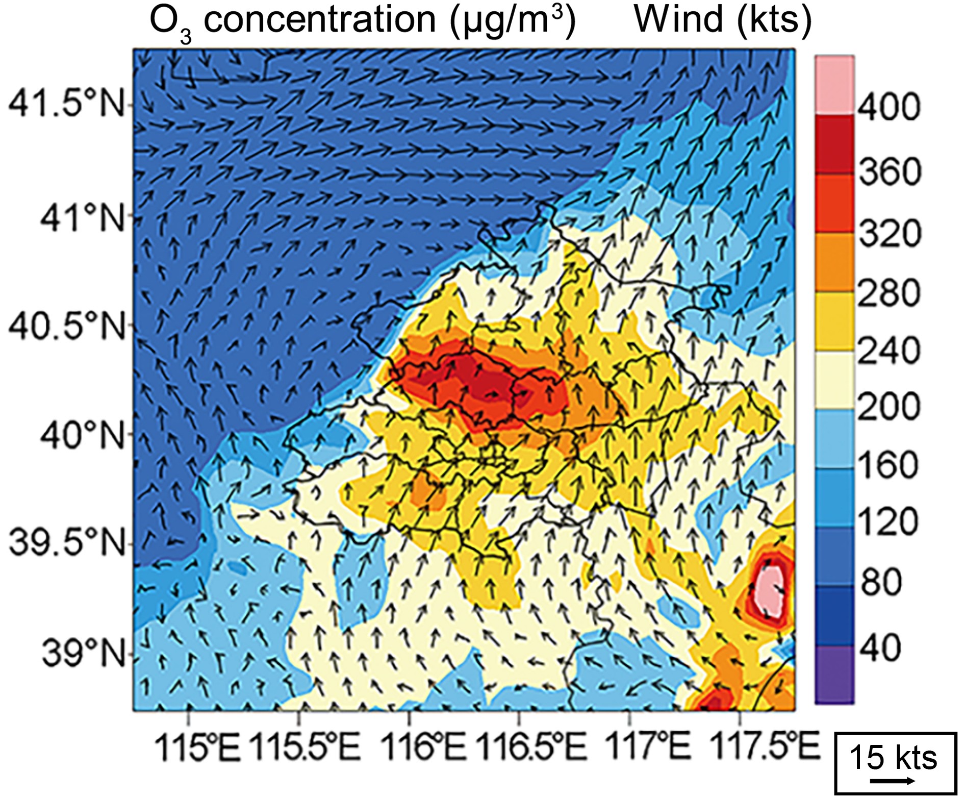
Figure 5 shows the 10 m wind field and ozone concentration simulated by the WRF-chem model at the peak time (1300 LST 18 May) in Beijing. The surface wind field in Beijing was dominated by southerly winds, which converged in the direction of the Taihang Mountain to the west. The wind field in the main urban area of Beijing was southeasterly, blowing pollutants from the urban area to Changping and Shunyi, where the wind speed slowed down and converged, resulting in ozone accumulation. At the same time, the solar radiation increased, and accordingly the temperature and ozone concentration increased significantly. For example, the ozone concentration in Changping exceeded 360 µg m^–3.

Figure 5.  Simulated 10m wind field and ozone concentration at 1300 LST 18 May 2017 (1 kt=1.852 km h⁻¹)

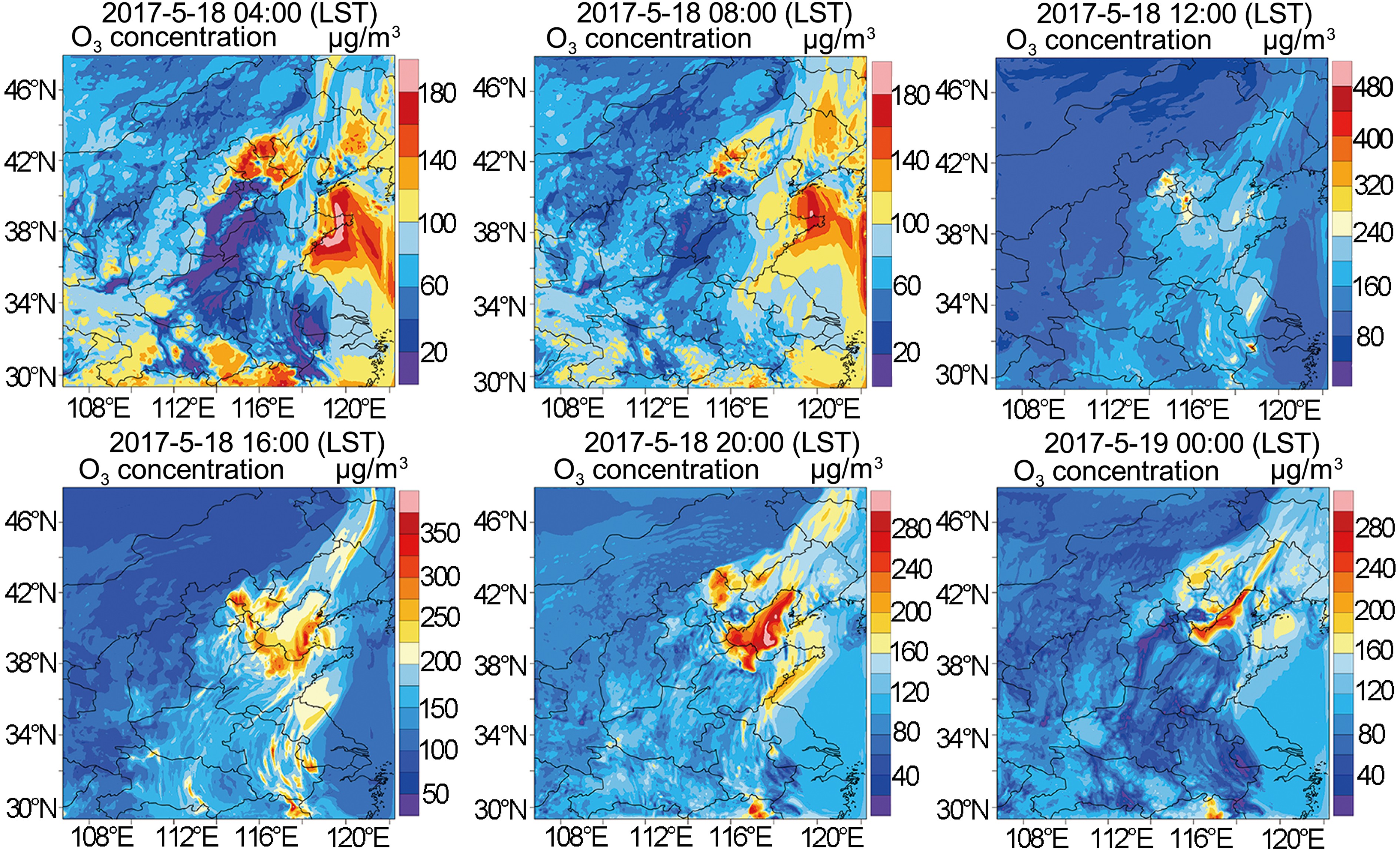
The spatial distribution of O₃ concentration from 0400 LST 18 to 0000 LST 19 May 2017 is simulated in Fig. 6. Taking the data on the 18th, when O₃ pollution was the most serious, as an example, we note that the long-distance transport process can be clearly seen in the spatial distribution, including an enhanced O₃ conveyor belt on the eastern side of Taihang Mountain. At 0400 LST on the 18th, the largest value of O₃ pollution area corresponded to the northern part of the Yellow Sea in eastern Shandong and northern Hebei.

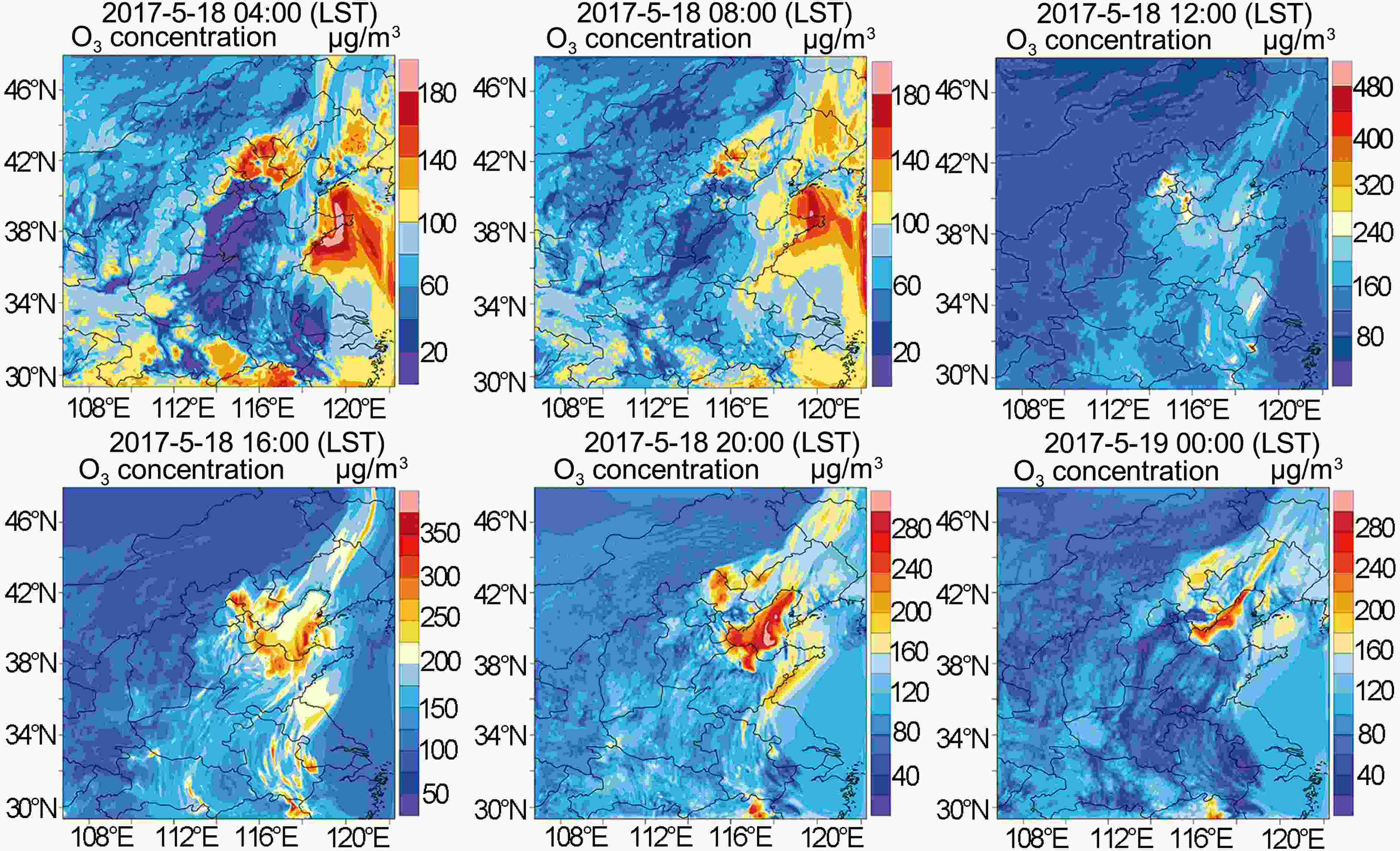
Figure 6.  Spatial distributions of simulated O₃ concentration from 0400 LST 18 to 0000 LST 19 May 2017.

The O₃ concentration in Beijing was ~140 µg m^–3, but the O₃ value in southeast Beijing was lower than to the northwest. At 0800 LST on the 18th, the peak amount of NO and VOC_S in the morning was followed by a drop of O₃ concentration to the northwest of Beijing but a slight rise in the southeast. At 1200 LST on the 18th, with the enhancement of solar radiation, the overall O₃ concentration in North China increased, and high O₃ values were found in Beijing, Tianjin and the Yangtze River delta. The maximum concentration of O₃ in Beijing was 320−360 µg m^–3, and the ozone concentration in the Yangtze River delta even exceeded 480 µg m^–3. At 1600 LST on the 18th, O₃ was transported a long distance, with O₃ flowing to the eastern side of Taihang Mountain causing the ozone pollution in the Yangtze River Delta to shift to the Yellow Sea, and the pollutants in northern Shandong advancing to the Bohai Sea region, thus resulting in the O₃ concentration in Beijing decreasing. At 2000 LST on the 18th, the high O₃ value area continued to move to the north. The pollution concentration in Beijing dropped to about 60−160 µg m^–3, and the concentration in Bohai Sea was higher than 300 µg m^–3. At 0000 LST on the 19th, the O₃ concentration in the southeast area of Beijing declined to 20−40 µg m^–3, and that in the northwest down to 140−160 µg m^–3.

Sensitivity of O₃ concentration to its precursor varies with the degree of emission disturbance, and moderate precursor reduction can effectively distinguish NO_x and VOC_S sensitivity (Sillman, 1999; Ye et al., 2016). In this paper, the sensitivity test is mainly carried out for the data on 18 May 2017, which is a day with the heaviest pollution. We adopted a 25% emission source disturbance, which distributes all NO_x or VOC_S species linearly in time and space.

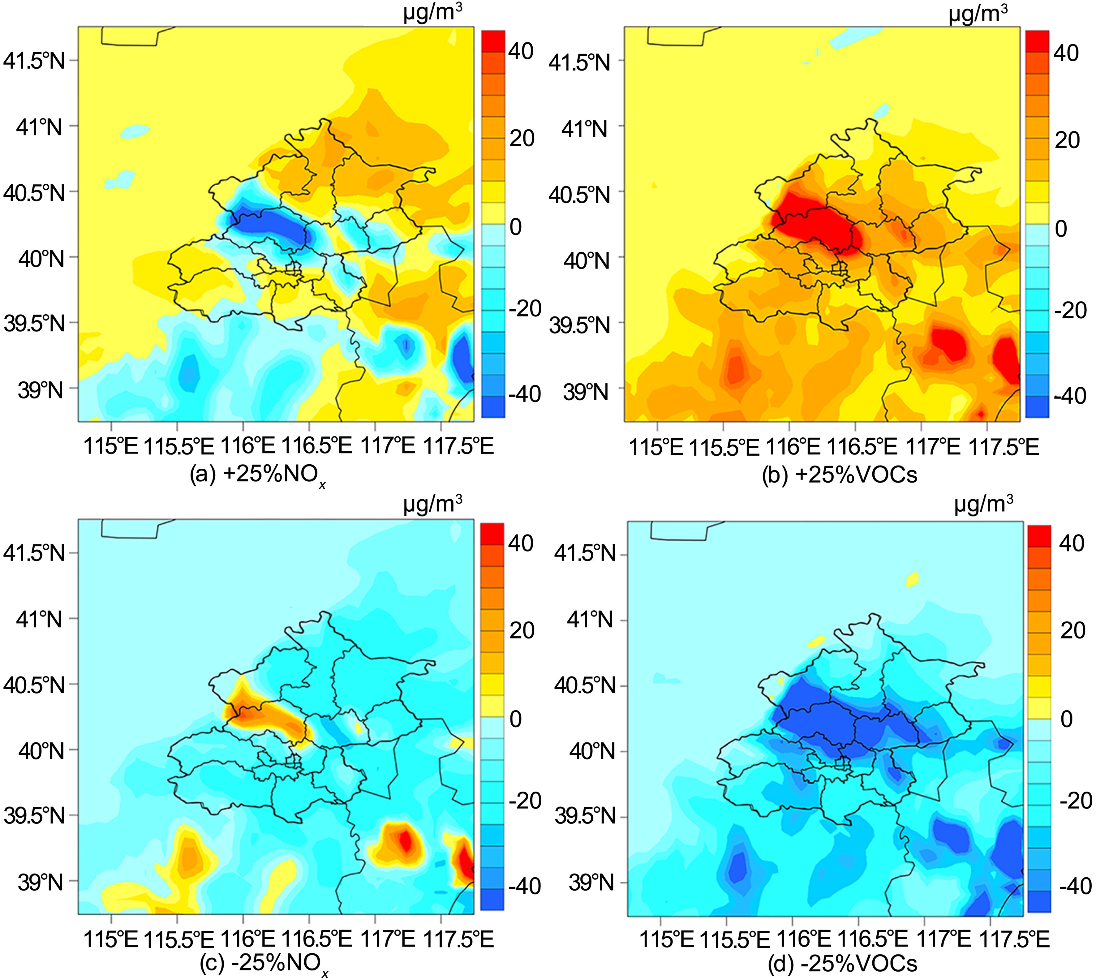
Figure 7 shows the variation of surface ozone concentration at the peak time (1300 LST on 18 May) with composite pollution caused by reducing and increasing precursors (NO_x and VOCs). Through sensitivity tests, we see that when NO_x increased by 25% (Fig. 7a), the ozone concentration declined at the peak time in central Beijing (including to the north of the main urban area, Changping, to the south of Yanqing, and the south of Pinggu, Shunyi and Tongzhou districts), the central Tianjin region and to the south of Hebei (including Baoding and Langfang region), of which Changping of Beijing saw the highest reduced value of 55.8 µg m^–3. This is because when NO_x is increased, NO reacts with O₃ to produce NO₂, which consumes O₃, resulting in a decrease in ozone concentration.

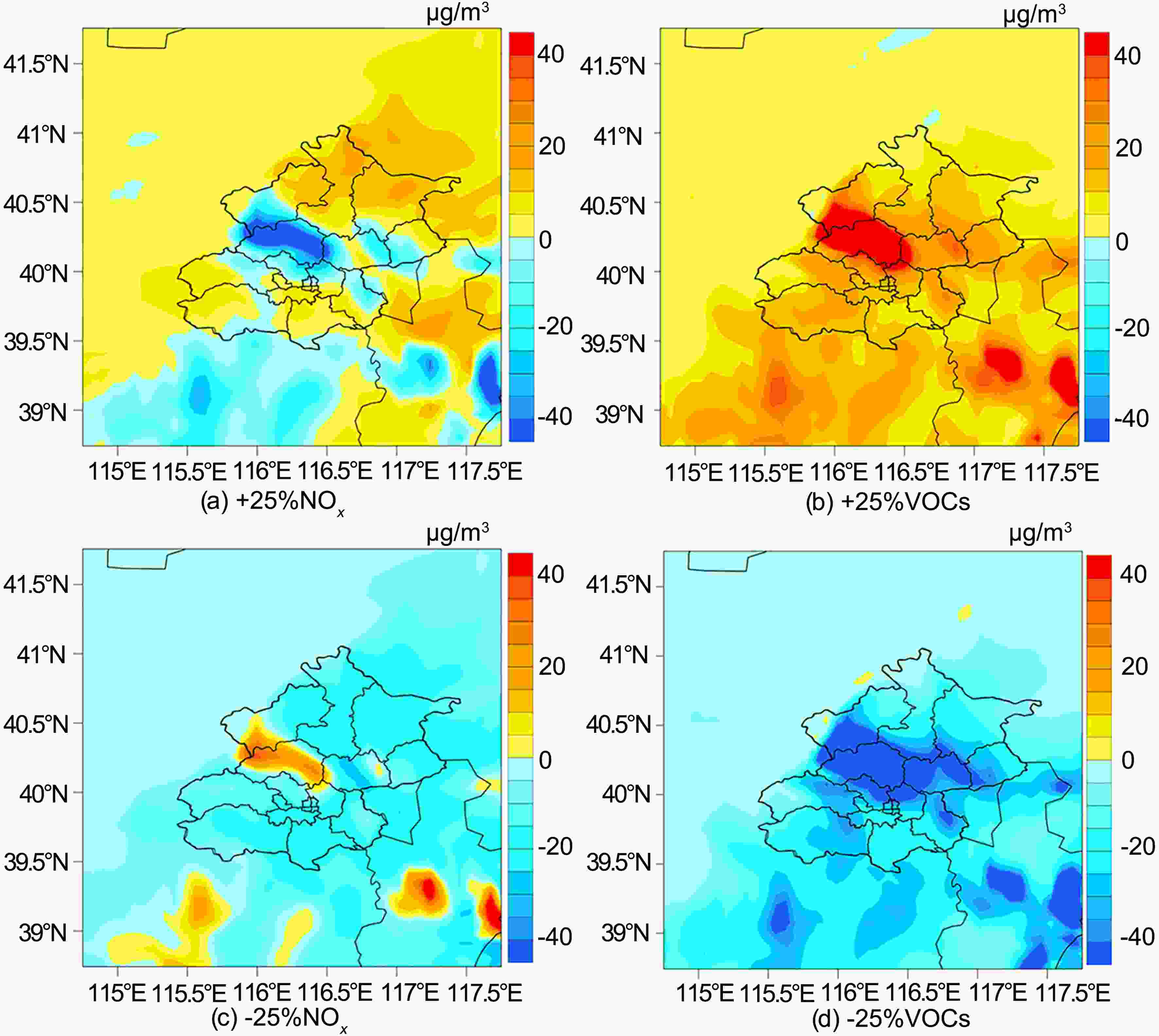
Figure 7.  Changes in surface ozone concentration caused by reducing and increasing precursors at the peak time of ozone (1300 LST 18 May). (Positive value means the increase of precursor concentration and negative value means the decrease of concentration)

Ozone concentration in other parts of Beijing (to the south of the main urban area, Huairou, Miyun, the north of Yanqing, Daxing and the east of Fangshan), the northern Tianjin and northern Hebei increased clearly at peak time, among which the ozone in the northern Huairou of Beijing was increased most significantly. When VOCs were increased by 25% (Fig. 7b), the peak ozone concentration in Beijing, Tianjin and Hebei increased too, and the ozone concentration in Changping of Beijing increased most significantly by 79.6 µg m^–3. When NO_x was reduced by 25% (Fig. 7c), the ozone concentration in other areas decreased except Changping, central Tianjin and parts of Hebei. This basically reflects an opposite trend to the change of ozone concentration increased by 25%, noting that the ozone concentration in Changping increases by about 24 µg m^–3. With 25% of VOCs reduced (Fig. 7d), the peak ozone concentration in Beijing, Tianjin and Hebei all decreased, showing an opposite trend to the change of ozone concentration resulting from an increase of 25% VOCs, with the ozone concentration in Changping decreasing most significantly by 104 µg m^–3.

Simulation results show that when the proportion of precursors (NO_x and VOCs) is reduced and increased by 25% respectively, the reduction of VOCs by 25% has the most significant effect on ozone concentration reduction at peak time. Among them, the central Beijing, central Tianjin and southern Hebei are VOCs-limited areas, and northeastern Beijing (northeast of Huairou and north of Miyun) is NO_x-limited region. Other areas such as southeast Beijing, northern Tianjin and northern Hebei are transitional sensitive areas.

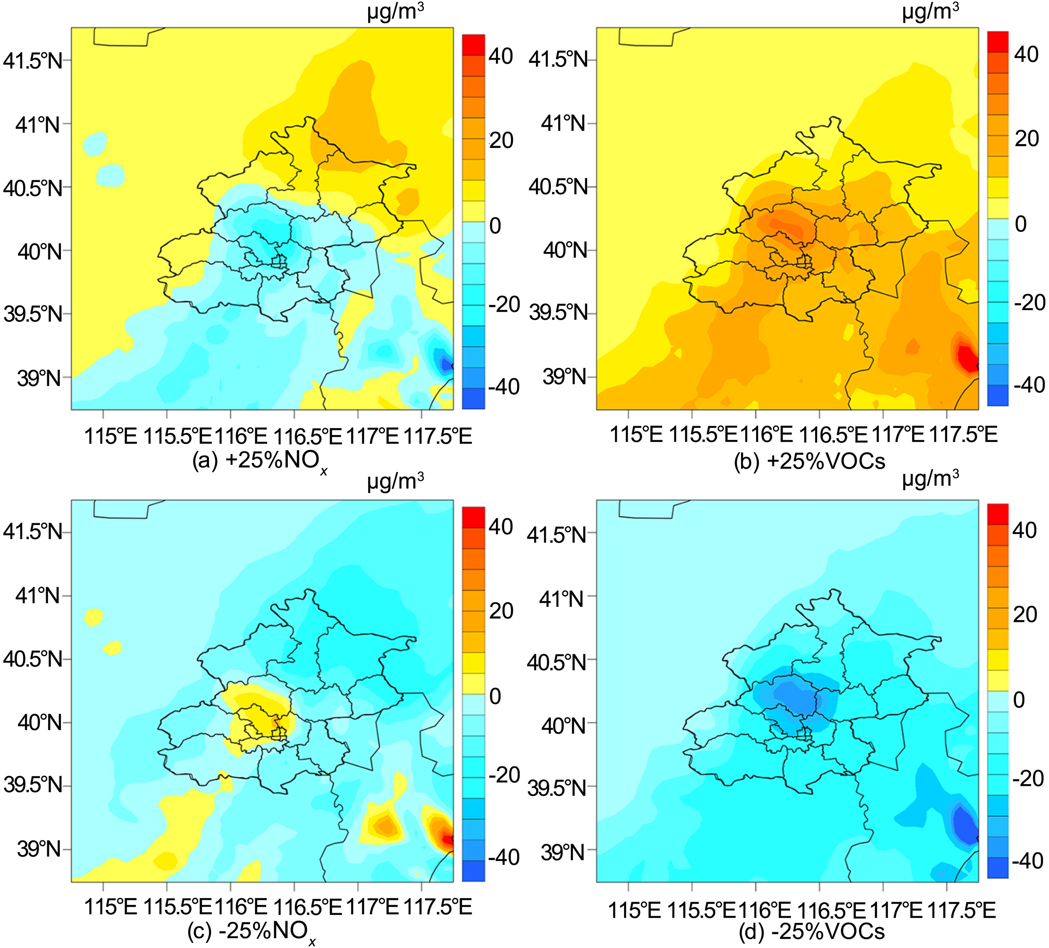
Figure 8 shows the average variation of surface ozone concentration during 0800−2000 (daytime) LST 18 May by reducing and increasing precursors (NO_x and VOCs). According to these sensitivity tests, when NO_x was increased by 25% (Fig. 8a), the average concentration of ozone in most areas of Beijing (main urban area, Changping, southern Yanqing, Shunyi, Tongzhou, Daxing, Fangshan and eastern Mentougou), central Tianjin and southern Hebei (Baoding, Langfang) decreased during the daytime, while in other areas the average concentration of ozone increased during the daytime. When VOCs were increased by 25% (Fig. 8b), the daytime average ozone concentration in Beijing, Tianjin and Hebei increased from 0800 to 2000 LST, with Changping of Beijing having the most significant increase. In contrast, when NO_x was reduced by 25% (Fig. 8c), the average ozone concentration in daytime decreased in most areas except the central part of Beijing (the northwest of main urban, the Changping and east of Mentougou), central Tianjin and a small part of Hebei. The change of average ozone concentration in most areas was opposite to that of increasing NO_x by 25%. When VOCs was reduced by 25% (Fig. 8d), the average ozone concentration in Beijing, Tianjin and Hebei decreased during the daytime, which basically shows an inverse trend to the change of ozone concentration with 25% VOCs increased, among which the average daytime ozone concentration in Changping area decreased most significantly.

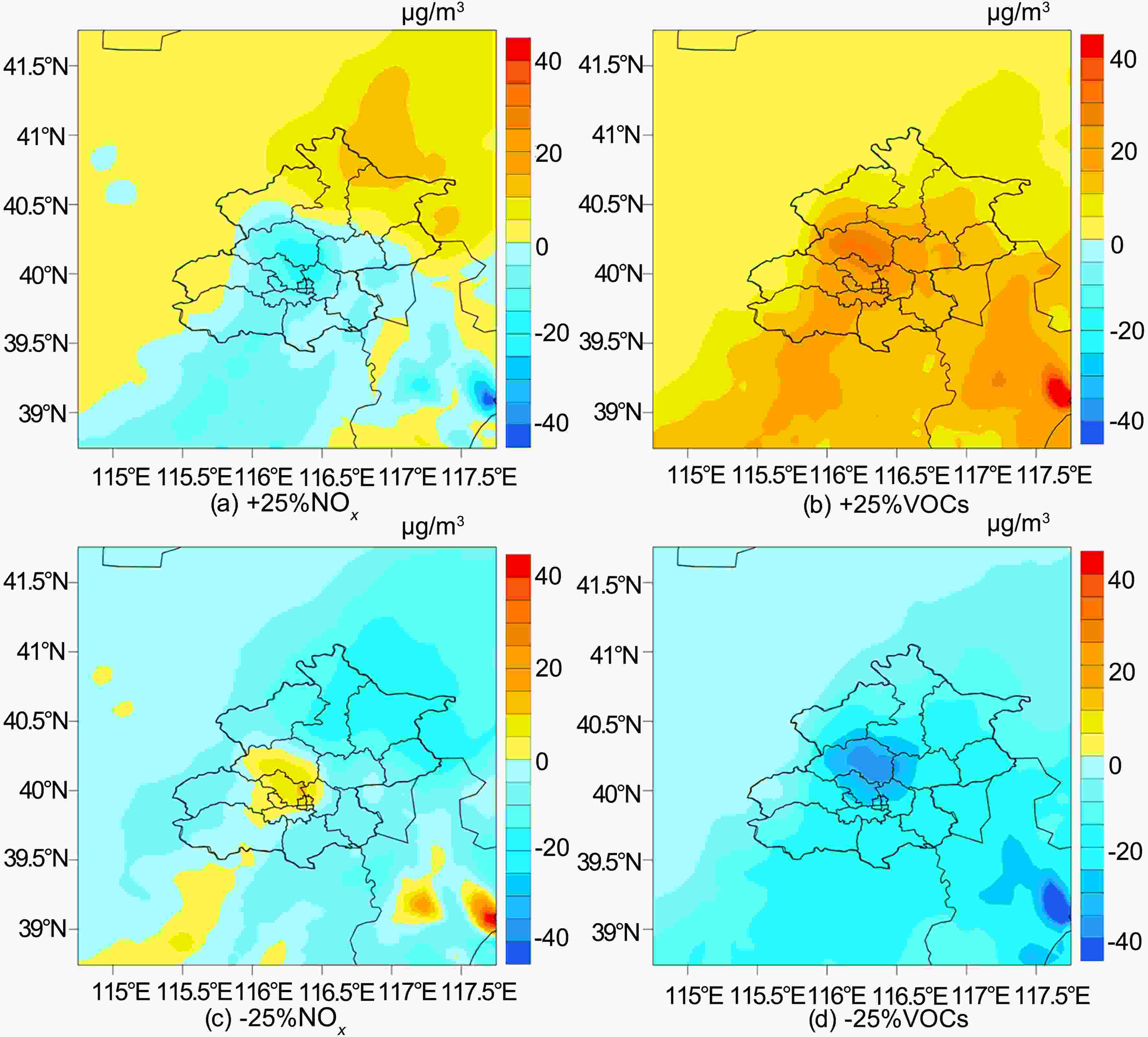
Figure 8.  The average change in surface ozone concentration caused by reducing and increasing precursors during the daytime from 0800 to 2000 LST 18 May 2017. (Positive value means the increase of precursor concentration and negative value means the decrease of concentration)

It can be seen from the above that when the proportion of precursors (NO_x and VOCs) is reduced or increased by 25%, the reduction of VOCs by 25% has the most significant effect on the average ozone concentration during the daytime on 18 May. Central Beijing (the north of main urban and Changping district), central Tianjin and southern Hebei (Baoding) belong to VOCs-limited areas, northeastern Beijing (northeastern Huairou and northern Miyun) are in the NO_x-limited areas, and other regions including northern Tianjin and northern Hebei are the transitional sensitive areas.

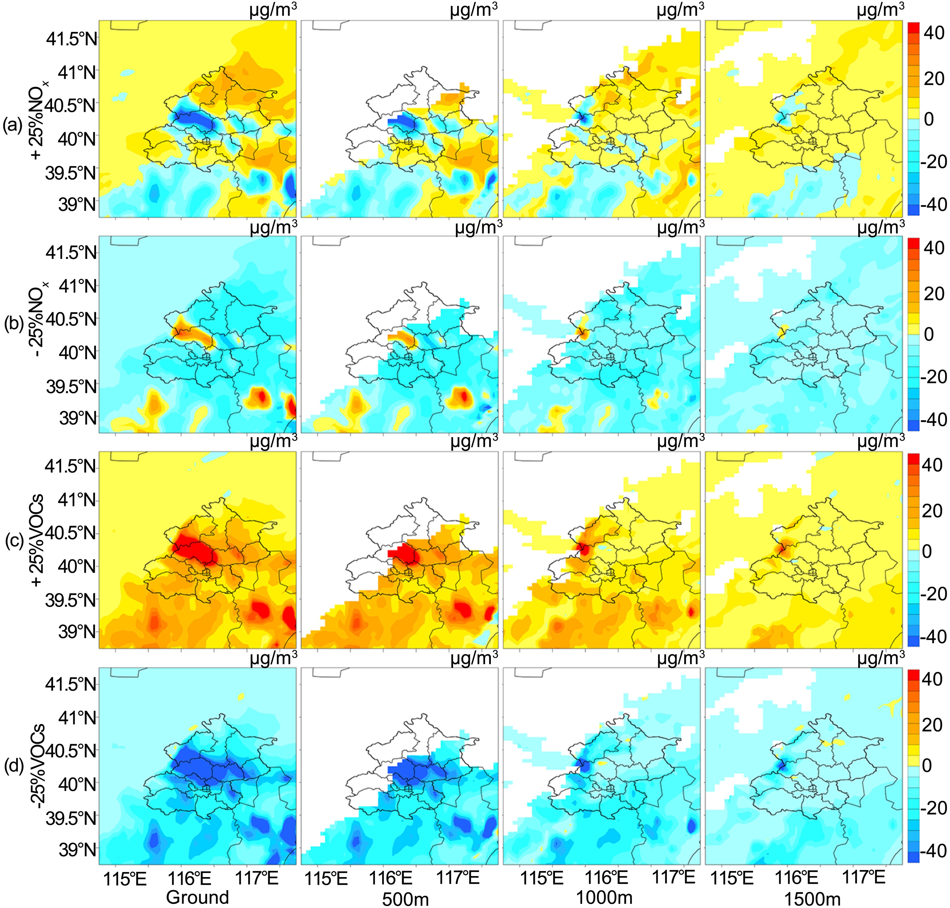
Figure 9 illustrates the change of ozone concentration at different heights at the peak time (1300 LST on 18 May). The first row from left to right of the picture shows the changes of ozone concentration at different heights (ground, 500 m, 1000 m and 1500 m) where NO_x is increased by 25% at peak time, while the second row shows the changes of ozone concentration at different heights where NO_x is reduced by 25%. The third row exhibits the changes of ozone concentration with VOCs increased by 25% and the fourth row shows that when VOCs is reduced by 25% at peak time. We can see that the change of ozone concentration weakens with increasing height, the position of the maximum and minimum of ozone concentration changes shifts westward, and the range decreases, moving from Shunyi and Changping to the east of Changping. With increasing height, the anthropogenic emissions of VOCs decrease, the sensitivity of VOCs becomes weaker, and the sensitivity of NO_x is enhanced. So, the VOCs-limited area decreases, becoming NO_x-limited.

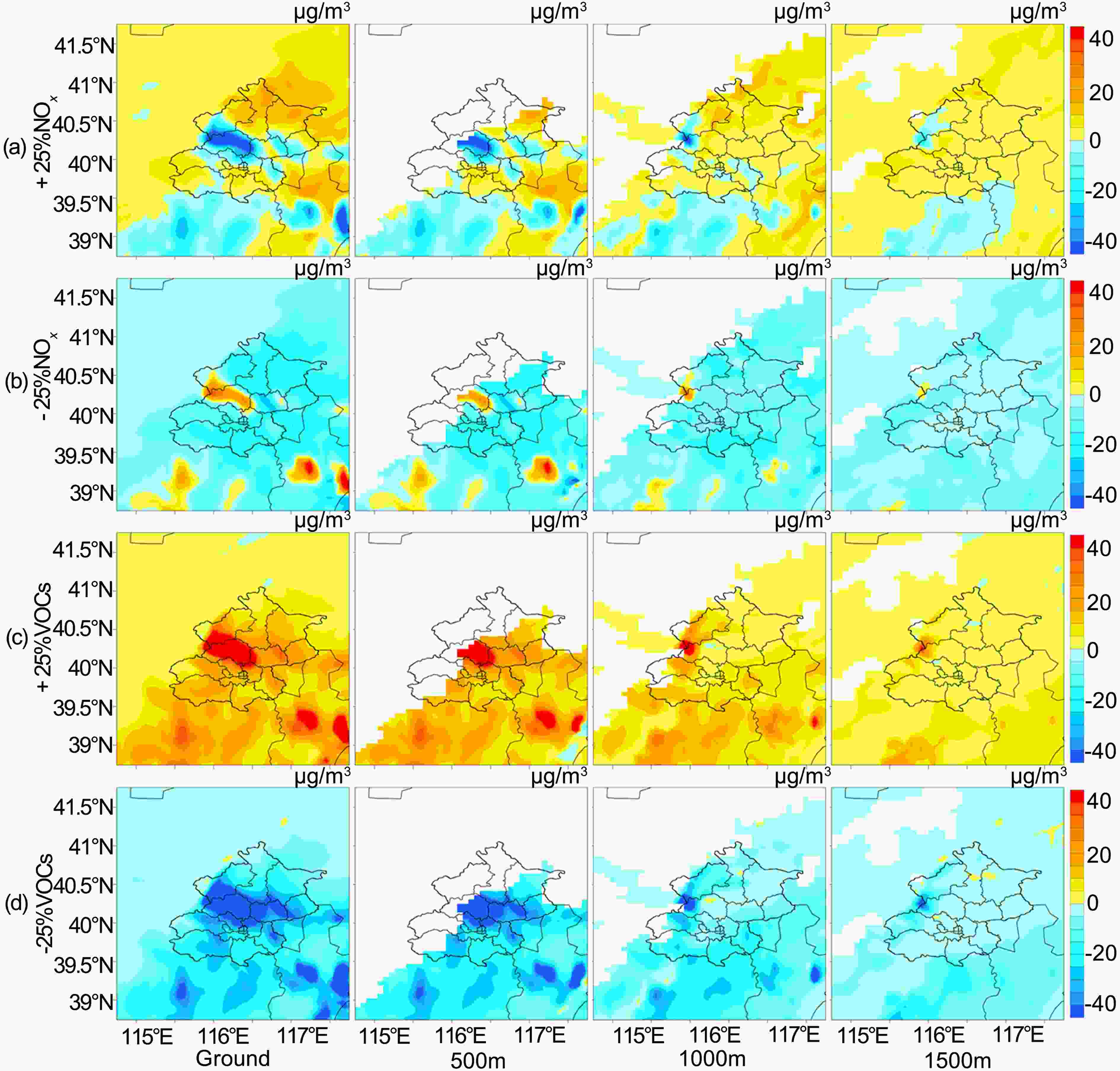
Figure 9.  Ozone concentration changes at different heights (surface, 500 m, 1000 m and 1500 m) at the peak time of ozone (1300 LST 18 May). (a) + 25% NO_x, (b) −25% NO_x, (c) + 25% VOCs, (d) −25% VOCs (Positive value means the increase of precursor concentration and negative value means the decrease of concentration).

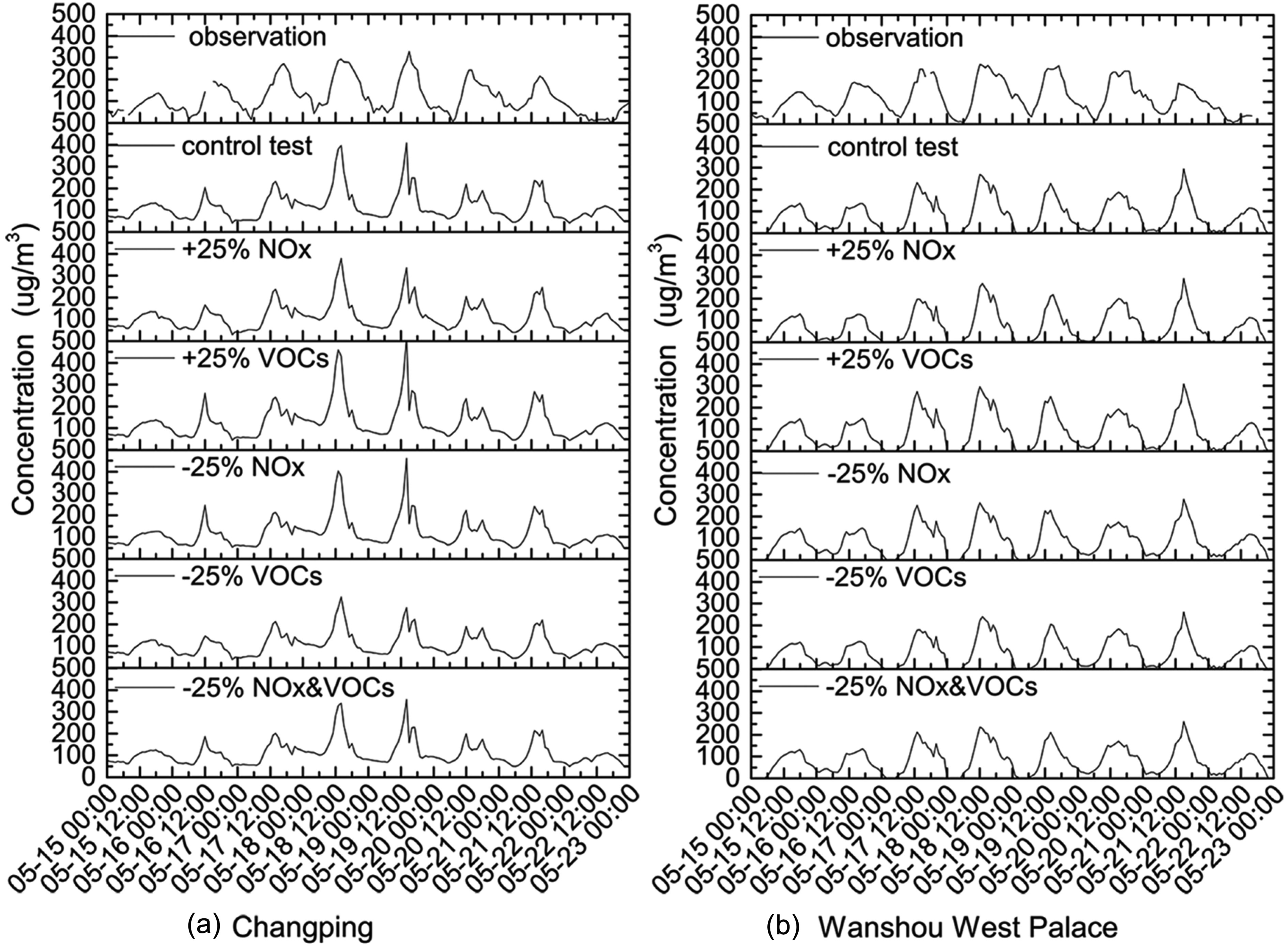
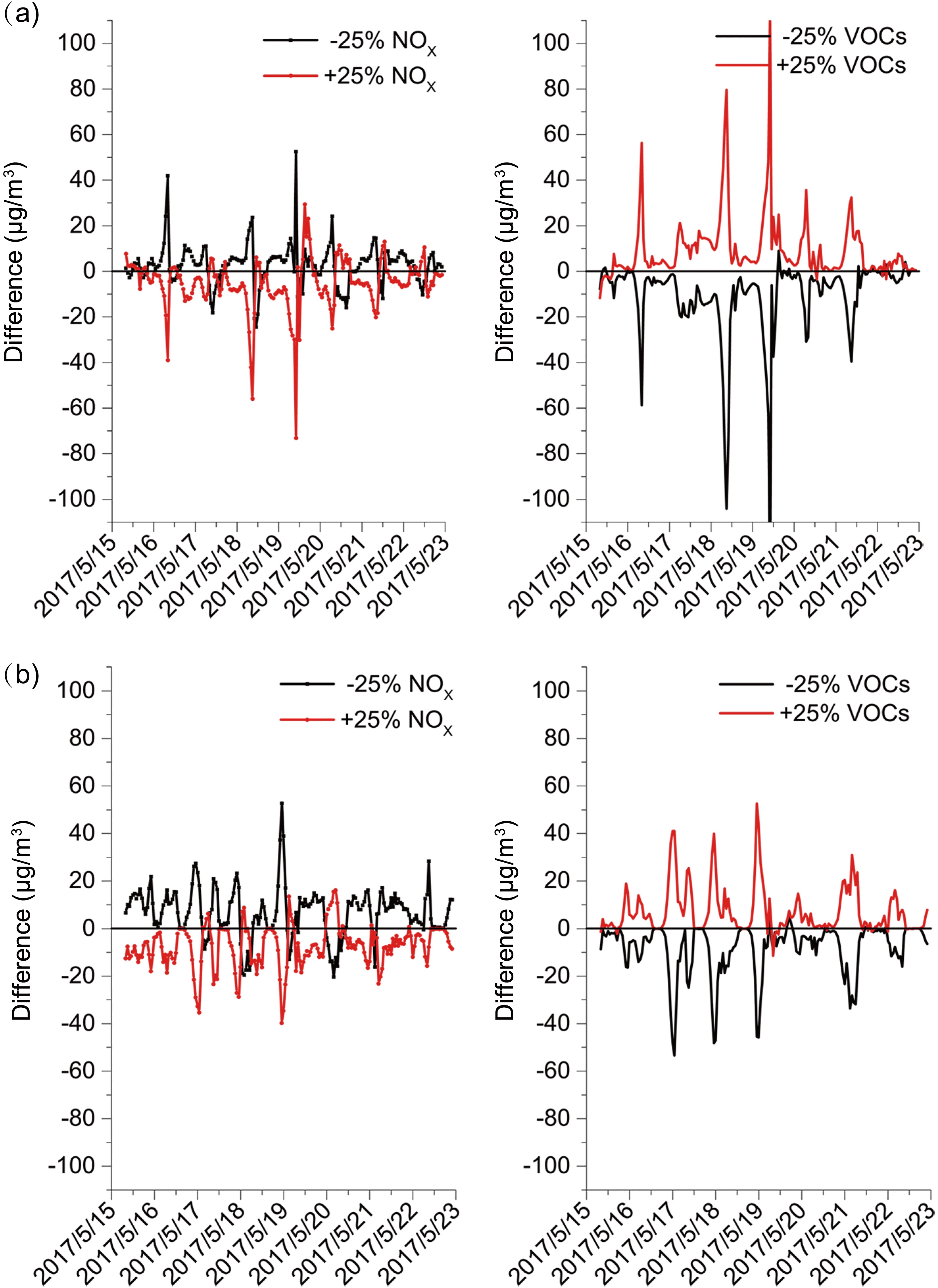
Figures 10 and 11 depict comparison graphs of variation and difference of ozone concentration in sensitivity tests of suburban (Changping) and urban areas (Wanshou West Palace). It can be seen that Changping is in an obvious VOCs-limited area (Figs. 10a and 11a), and the concentration of O₃ at peak time (1300 LST 18 May) varies in a decreasing trend: +25% VOCs (460.0 µg m^–3) > −25% NO_x (404.1 µg m^–3) > control test (380.4 µg m^–3) > −25% NO_x & VOCs (328.5 µg m^–3) > +25% NO_x (324.6 µg m^–3) > −25% VOCs (276.3 µg m^–3). In other words, the increase or reduction of VOCs has a more significant impact on the peak concentration of O₃ than NO_x. The increase of VOCs and the reduction of NO_x enhance the ozone concentration, while the increase of NO_x and the reduction of VOCs diminish the ozone concentration. For the discussed ozone pollution process, the reduction of 25% NO_x increased the ozone concentration by 23.7 µg m^–3 at the peak time, while the reduction of 25% NO_x and VOCs reduced the ozone concentration by 51.9 µg m^–3, and the reduction of 25% VOCs reduced the ozone concentration by 104.1 µg m^–3. Changping achieved the best emission reduction effect by cutting 25% VOCs at the peak time, which is twice as effective as the reduction of 25% NO_x and 25% VOCs.

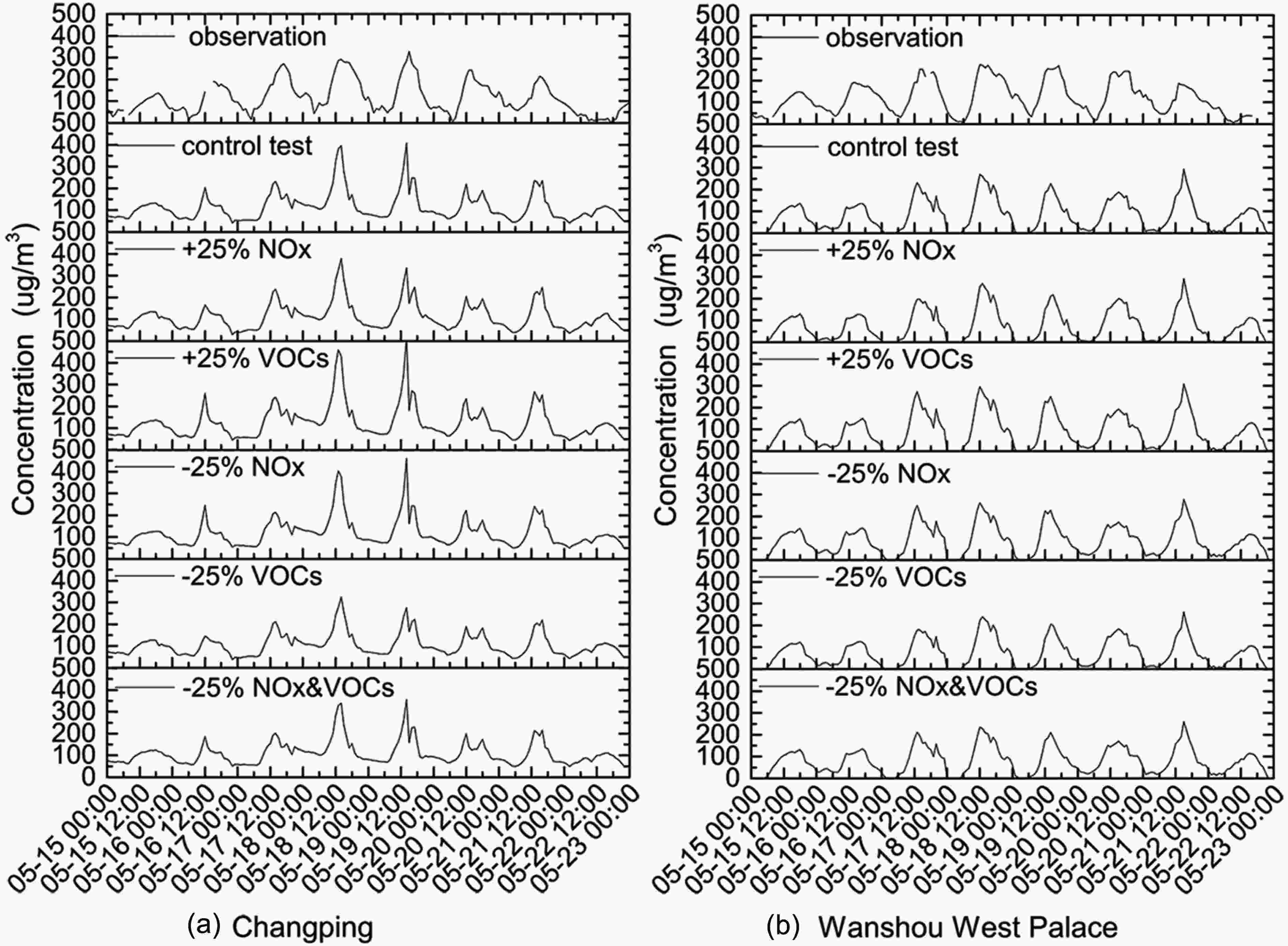
Figure 10.  Comparison of ozone concentration changes in the sensitivity tests from 16 to 23 May 2017. (a) Changping Station, (b) Wanshou West Palace Station

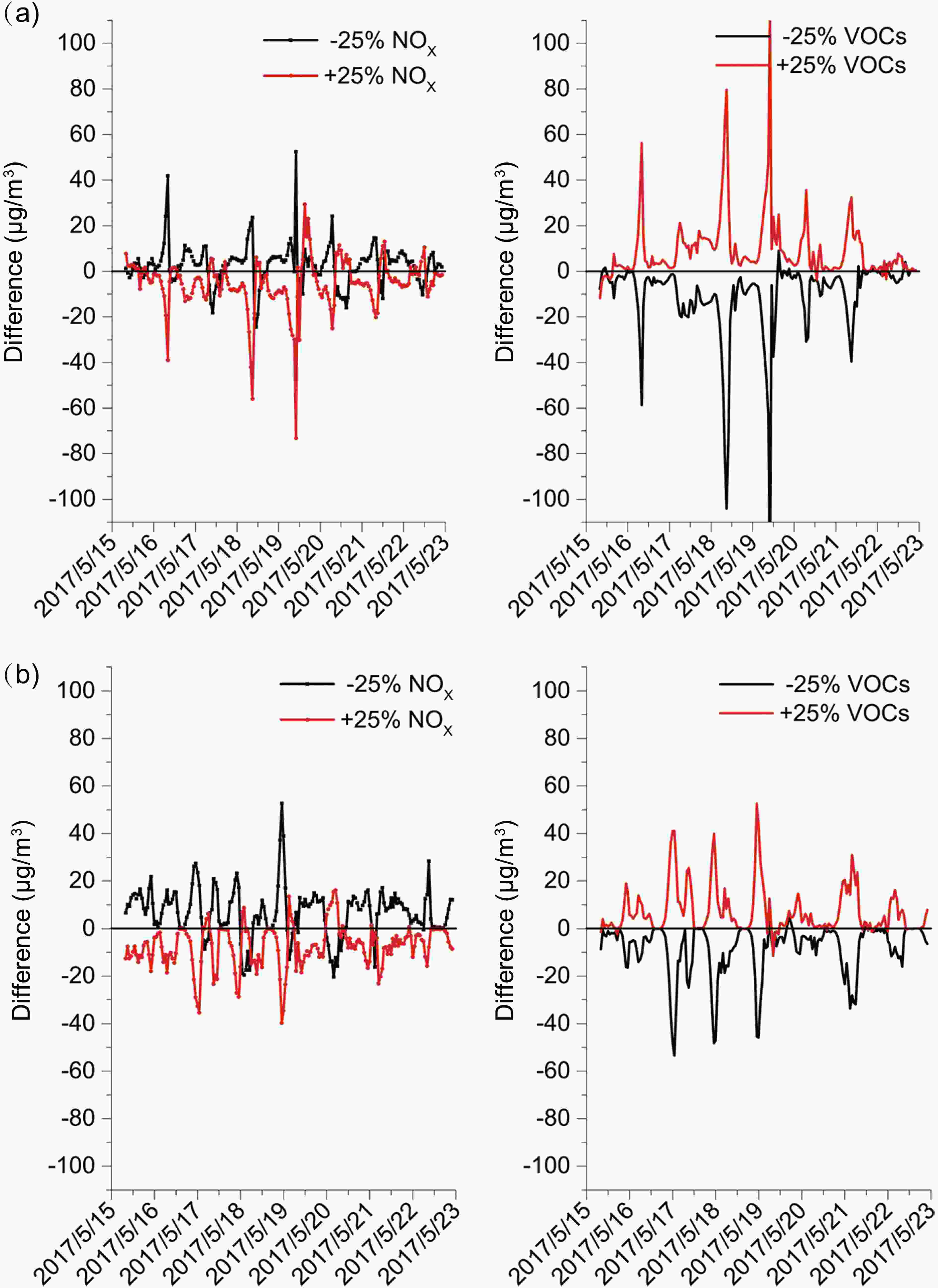
Figure 11.  Comparison of ozone concentration differences in sensitivity tests from 16 to 23 May 2017. (a) Changping Station, (b) Wanshou West Palace Station.

The O₃ concentration at Wanshou West Palace Station at peak time (1300 LST 18 May) (Figs. 10b and 11b) also varies decreasingly: +25% VOCs (273.6 µg m^–3) > control test (272.6 µg m^–3) > +25% NO_x (269.2 µg m^–3) > −25% NO_x (243.2 µg m^–3) > −25% VOCs (239.7 µg m^–3) > −25% NO_x&VOCs (229.3 µg m^–3). The increased VOCs and reduced NO_x heighten the ozone concentration, but the increased NO_x and reduced VOCs weaken the ozone concentration. Increasing or reducing VOCs has a more significant effect on O₃ peak concentration than NO_x. The reduction of 25% NO_x and 25% VOCs reduced ozone concentration by 29.4 µg m^–3 and 32.9 µg m^–3, respectively, and the reduction of 25% NO_x and 25% VOCs together reduced ozone concentration by 43.3 µg m^–3. The combined reduction of 25% in NO_x and VOCs is better than the only 25% reduction in VOCs. The concentration difference of sensitivity test for Wanshou West Palace Station (urban site) was smaller than that for Changping (suburban site), and the sensitivity was not as obvious as that at Changping Station.

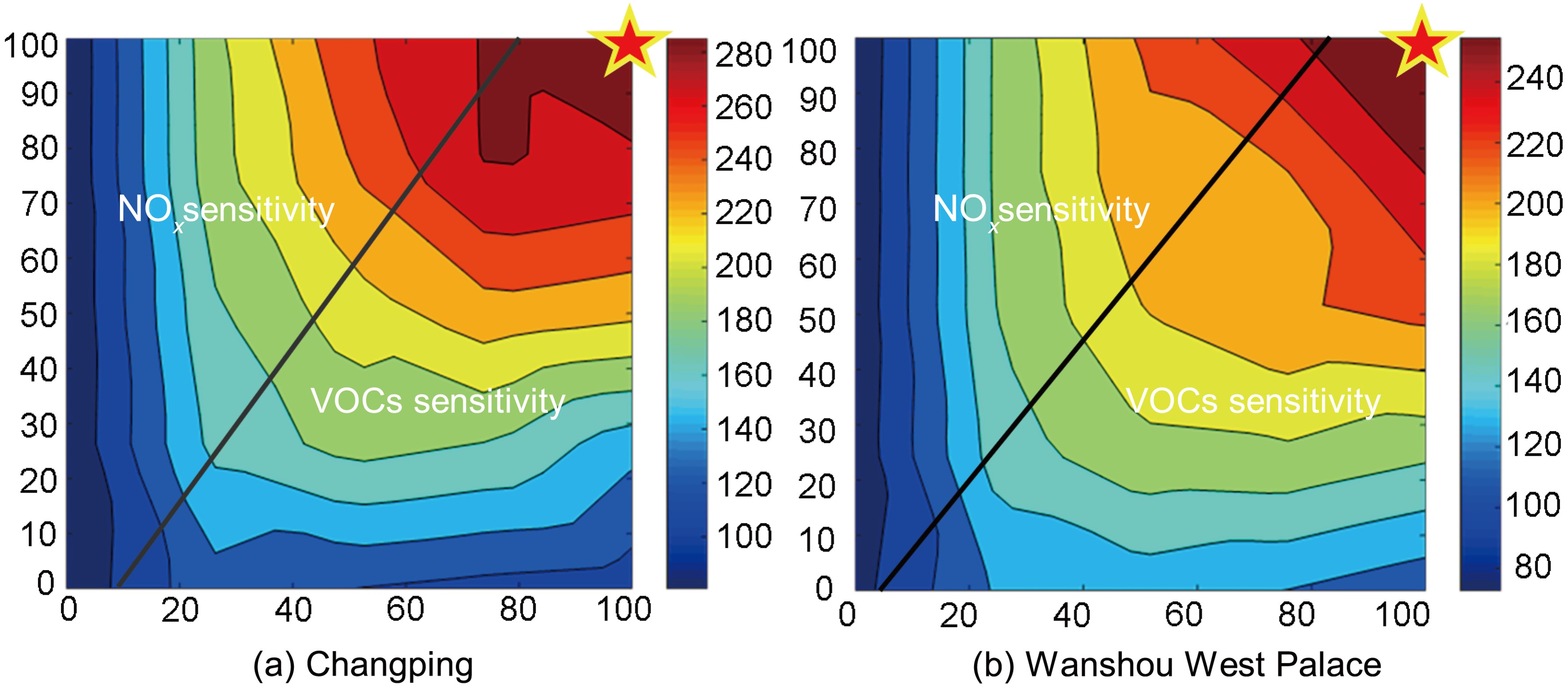
Figures 12a and 12b are the EKMA curves drawn by selecting the peak concentration in the suburbs (Changping) and the urban area (Wanshou West Palace) on 18 May 2017. The vertical axis is the percentage of the original VOCs, the horizontal axis is the percentage of original NO_x, and the red five-pointed star in the upper right corner is the control test without reduction (accounting for 100% NO_x and 100% VOCs). Based on the red star in the upper right corner, it can be seen from the EKMA curve that the daily peak concentration of ozone is not a simple linear relationship with precursors (NO_x, VOCs). Connecting the turning points of ozone concentration isolines into a line is called the ridge line of EKMA curve. NO_x sensitivity is on the left side of the EKMA ridge line and VOCs sensitivity on the right side. The ratio of VOCs/NO_x affects the distribution of the EKMA ridge line. In the sensitive area of VOCs, when the initial concentration of fixed VOCs remains unchanged and the initial concentration of NO_x is changed, the daily maximum concentration of ozone changes little; when the initial concentration of fixed NO_x is unchanged and the initial concentration of VOCs increases, the daily maximum concentration of ozone increases significantly, that is, the ratio of VOCs/NO_x is small. In the NO_x sensitive area, when the initial concentration of fixed VOCs is unchanged and the initial concentration of NO_x is increased, the daily maximum concentration of ozone increases significantly; when the initial concentration of fixed NO_x is unchanged and the initial concentration of VOCs is changed, the daily maximum concentration of ozone does not change significantly, which means the ratio of VOC_S/NO_x is larger.

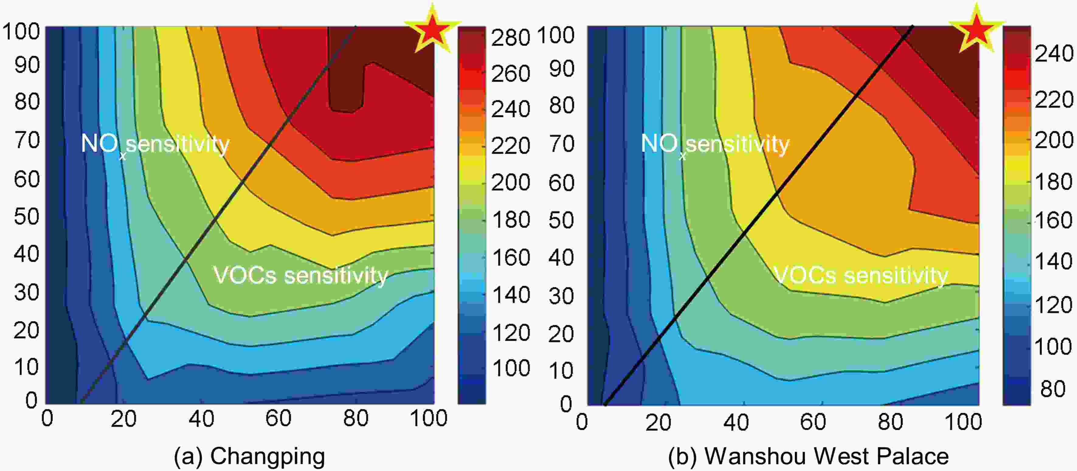
Figure 12.  EKMA curves of Beijing suburban station (Changping) and urban station (Wanshou West Palace) under different weather conditions. The vertical axis is the percentage of the original VOCs, the horizontal axis is the percentage of original NO_x, and the red five-pointed star in the upper right corner is the control test without reduction (accounting for 100% NO_x and 100% VOCs).

Figure 12 indicates that the EKMA curve based on model simulation reflects the photochemical reaction process of precursors with different initial concentrations, and how the sensitivity of Beijing suburbs (Changping) and urban areas (Wanshou West Palace) is divided into VOCs sensitivity. That is, when NO_x and VOCs emissions are reduced by the same proportion, VOCs reduction will cause O₃ concentration to decrease more, and reducing the initial concentration of NO_x by a certain proportion will increase O₃ concentration. Comparing EKMA curves of suburban (Changping) and urban areas (Wanshou West Palace), we find that ozone concentration in the suburbs is always higher than that in urban area. The slope of the ridge line of EKMA curve is larger in the suburbs and VOCs-limited area in the suburbs is larger than that in urban areas. When the VOCs/NO_x ratio is small, the reaction rate of NO_x and OH is faster than that of VOCs and OH (Sinha et al., 2012), and the excessive emission of NO_x contributes to the fact that VOCs is the key to control the balance of ozone reaction. Therefore, controlling VOCs emissions can control excessive ozone pollution. As the exeedance concentration of O₃-1h is 200 µg m^–3, in order to make O₃-1h attain the standard and minimize the emission reduction cost of precursors (NO_x and VOCs), the stations in the suburbs (Changping) and the urban areas (Wanshou West Palace) are all in the VOC_S-limited area, so it is necessary to reduce the emission of VOCs to control the ozone pollution in Beijing.

According to the exceedance concentration of O₃-1h and the emission reduction cost of precursors (NO_x and VOCs), the following emission reduction schemes are formulated for the pollution process: O₃-1h concentration can reach the standard when 60% VOCs are reduced in the suburbs (Changping), and O₃-1h concentration can reach the standard when 50% VOCs are reduced in the urban areas (Wanshou West Palace).

The WRF-Chem model successfully simulated the combined pollution process of ozone and haze formation from 13 to 23 May 2017. The simulation results could provide some references for the air quality forecast and early warning in Beijing. Upon either reducing or increasing the proportion of precursors (NO_x and VOCs) by 25% at the same time, it was found that the reduction of VOCs by 25% had the most significant effect on the average concentration of ozone. When VOCs and NO_x were reduced by the same proportion, the reduction effect of O₃ was more obvious at peak time, and the effect in the daytime was more obvious than that at night. Compared with the results of precursor sensitivity test, the obvious change in ozone concentration is: peak time > daytime average. When the proportion of precursors (NO_x and VOCs) was reduced and increased, respectively, by 25%, the changing characteristics of ozone concentration in the vertical was found to decrease with increasing height, and the position of the maximum area of ozone concentration change shifted westward and its range narrowed. With increasing height, VOCs-limited area decreased, VOCs sensitivity decreased and NO_x sensitivity increased. The control area changed from VOCs-limited near the surface to NO_x-limited at high altitudes.

Using the WRF-Chem model combined with the empirical kinetic modeling method (EKMA curve) to study the sensitivity of ozone precursors in the process of complex pollution, we have found that both suburban (Changping) and urban areas (Wanshou West Palace) are sensitive to VOCs. According to the results of sensitivity test, the following emission reduction schemes are formulated: during the pollution process on 18 May 2017, when it is reduced by about 60% VOCs in the suburban area (Changping), the O₃-1h concentration can reach the standard, and when it is diminished by about 50% VOCs in the urban area (Wanshou West Palace), the O₃-1h concentration can reach the standard.

Acknowledgements. This study is funded by Air Pollution Special Project of the Ministry of Science and Technology (Grant No. 2017YFCOZ10006) and the National Natural Science Foundation of China (Grant No. 41975173)