


 DownLoad:


-
The initialization of hydrometeors plays a vital role in numerical weather prediction (NWP) due to their participation in the microphysical process related to clouds and precipitation (Errico et al., 2007; Bauer et al., 2011; Kerr et al., 2015). Various methods have been applied to improve the initialization of hydrometeors in NWP, such as the cloud analysis technique (Hu et al., 2006; Toth et al., 2012), the nudging-based technique (Huang et al., 2018; Wang et al., 2018) and some more advanced data assimilation techniques, like variational assimilation method (Sun and Crook, 1997; Xiao et al., 2007; Gao and Stensrud, 2012; Wang et al., 2013; Chen et al., 2015, 2016; Chen et al., 2020), Ensemble Kalman Filter (EnKF) technique (Tong and Xue, 2005; Dowell et al., 2011; Jones et al., 2013; Putnam et al., 2019), and the hybrid Ensemble-Variational (EnVar) method (Gao and Stensrud, 2014; Wang and Wang, 2017; Pan et al., 2018; Meng et al., 2019).
In the variational and EnKF-based data assimilation techniques, the analysis is obtained by finding a maximum likelihood of the probability density functions (PDFs) of the true state of atmosphere when observations and a priori background estimation are given. Common data assimilation systems theoretically require that the PDFs of analysis, background, and observation errors satisfy the Gaussian unbiased distribution. If the assumption is not satisfied, unrealistic analysis will arise in the data assimilation process (Errico et al., 2000; Ravela et al., 2007).
A non-Gaussian (NG) nature of the background errors could result from the time integration of the model nonlinearity (Bocquet et al., 2010), especially the highly nonlinear physical processes in NWP (Auligné et al., 2011). The displacement errors of meteorological features may also lead to NG in the background errors (Lawson and Hansen, 2005). Among the model variables which are commonly used in the data assimilation systems, hydrometeors tend to have the highest degree of nonlinearity and the lowest predictability (Fabry and Sun, 2010; Fabry, 2010). Thus, NG is inevitable when the control variables of data assimilation systems include hydrometeors, which is of vital importance for assimilating cloud sensitive observations, like radar reflectivity and cloudy satellite radiances (Errico et al., 2007).
Various studies have focused on how to include hydrometeors as control variables in the data assimilation systems in order to directly analyze hydrometeors from the cloud sensitive observations. The total water mixing ratio (TWMR), which is the sum of the humidity-related variable and hydrometeors, is used as the control variable in many studies (Xiao et al., 2007; Liu et al., 2009; Yang et al., 2016; Li et al., 2017). However, TWMR is indeed a humidity control variable, and it is often limited to the simple and incomplete microphysical process employed to separate the hydrometeor increments from the total humidity increments. Hydrometeor mixing ratios are also chosen as the control variables in some data assimilation systems (Gao and Stensrud, 2012; Wang et al., 2013; Chen et al., 2015). Hydrometeor mixing ratios are easy to implement in a data assimilation system, but the NG of the hydrometeor background errors has not been taken into consideration in past studies. Some other studies chose the logarithm of hydrometeor mixing ratios as the control variables in the data assimilation systems (Boukabara et al., 2011; Michel et al., 2011; Liu et al., 2020), but did not include a thorough discussion of the NG aspect of the logarithm of hydrometeors. Recently, some researchers have used reflectivity as the control variable in data assimilation system (Wang and Wang, 2017), but its application is limited to radar reflectivity assimilation with pure ensemble background error covariances. To obtain more Gaussian hydrometeor control variables, Hólm and Gong (2010) explored how to extend the humidity control variable transform method (Hólm, 2002) of the European Centre for Medium-Range Weather Forecasts (ECMWF) to include hydrometeors. In their research, the normalized hydrometeors were selected as the control variable candidates, but the exact formulation of the normalization was not given and needs further investigation.
In this study, a new Gaussian transform method is proposed with the objective to construct more Gaussian hydrometeor control variables in variational data assimilation systems. The new Gaussian transform is modified based on the Softmax function (Bridle, 1990), and is named the Quasi-Softmax function in this study. This article will be organized as follows. In section 2, the Quasi-Softmax method, the D′Agostino test (D′Agostino, 1970), the configuration of the experiments, and the description of statistical samples are presented. In section 3, the discussion of the transformed hydrometeors from the perspective of spatial distribution, NG and characteristics of background errors is given. Finally, the conclusions are drawn in section 4.
-
For a set of samples
${x_1},{x_2}, \cdots,{x_n}, \cdots,{x_N}$ , the normalization of their exponential functions are${{\rm{x}}_1},{{\rm{x}}_2}, \cdots,{{\rm{x}}_n}, \cdots,{{\rm{x}}_N}$ , where${{\rm{x}}_n}$ is defined asThis transformation is called the Softmax function (Bridle, 1990), which is commonly used in neural networks. The numerator of Eq. (1) is the exponential function of
${x_n}$ , and the denominator is the sum of the exponentials of all the samples; β is a parameter that controls the degree of increase in the contrast of the Softmax function. The Softmax function is a normalized exponential function and is often used in neural networks for classification problems. The Softmax function can be used to represent the probability of class membership for parameters with exponential distributions such as the Gaussian distribution (Bishop, 1995). The Softmax function has been employed to transform cloud fraction to a more Gaussian-like control variable in retrieving cloud fraction from satellite radiances (Auligné, 2014).Considering that the magnitude of hydrometeor mixing ratios is relatively small and the typical non-precipitation region may cover a large area, the calculated denominator in Softmax function may be very close at different levels, making it possible that the vertical distribution characteristics of hydrometeor mixing ratios may be lost after transformation. To handle this issue, a modification has been made to the Softmax function, renamed as the Quasi-Softmax function. With the Quasi-Softmax function, the original hydrometeor mixing ratio
${q_{i,j,k}}$ is transformed to${Q_{i,j,k}}$ :In Eq. (2),
${q_{i,j,k}}$ is the corresponding hydrometeor at the coordinate position$(i,j,k)$ , and${\bar q_{i,j}}$ is the average of the vertical profiles of hydrometeors at horizontal positions$(i,j)$ , which is defined as:where K is the number of vertical levels. Compared to the original Softmax function, the denominator of Quasi-Softmax function becomes the sum of the exponential function of
${\bar q_{i,j}}$ in certain areas rather than the whole model domain. The sum is calculated over an area where${\bar q_{i,j}}$ > 0 and${q_{i,j,k}}$ = 0. To increase the contrast after transformation, β is set to 100 for cloud water mixing ratio (${q_{\rm{c}}}$ ) and rain water mixing ratio (${q_{\rm{r}}}$ ), and 1000 for cloud ice mixing ratio (${q_{\rm{i}}}$ ) and snow mixing ratio (${q_{\rm{s}}}$ ). In this study, the Quasi-Softmax function is applied to the full variable states rather than the perturbations. -
The degree to which samples deviate from being truly Gaussian can be detected from the PDF’s skewness and kurtosis. The skewness measures asymmetry of the PDF about its mean, while kurtosis is a measure of how peaked is the distribution. For a given sample
${x_1},{x_2}, \cdots,{x_n}, \cdots,{x_N}$ , its skewness and kurtosis can be calculated as:where
${G_3}$ and${G_4}$ are the skewness and kurtosis of the sample, respectively, and$\bar x$ is the mean of the sample. For a Gaussian distribution, skewness is zero, whereas positive (negative)${G_3}$ values indicate a median of PDF that is smaller (larger) than its mean and with a large right (left) tail. The kurtosis will be 3 if the distribution is Gaussian, with larger tails and a narrow modal peak resulting in larger${G_4}$ values. Sample skewness and kurtosis can be used together to detect deviations from being exactly Gaussian, but in NWP, the ensemble number is relatively small (typically <100), making the normality of skewness and kurtosis often difficult to attain with sufficient accuracy (Thode, 2002). Therefore, we introduce the D′Agostin test (hereafter K2 test; D′Agostin et al., 1970) to diagnosis the degree of NG of samples. The K2 test is a univariate statistical test which combines the transformed skewness and kurtosis, and it can be used to test the NG of samples with number > 20 (Thode, 2002). In the K2 test,${G_3}$ and${G_4}$ are transformed to${f_3}({G_3})$ and${f_4}({G_4})$ , respectively, where${f_3}({G_3})$ is defined as:and
${f_4}({G_4})$ is defined asPositive (negative)
${f_3}({G_3})$ values mean that the PDF distribution of sample has a median smaller (higher) than the mean with a longer right (left) tail, while positive (negative)${f_4}({G_4})$ values indicate that the PDF has a larger (smaller) modal peak than the Gaussian distribution. Finally,${f_3}({G_3})$ and${f_4}({G_4})$ are combined to produce an omnibus test${K^2}$ :The
${K^2}$ (hereafter K2) is zero when the PDF of the sample is a Gaussian distribution. The higher the calculated K2 value is, the greater the NG of the sample will be. Legrand et al. (2016) used the K2 test to diagnose NG of forecast and analysis errors in a convective-scale model, and the NG of common variables relating to wind, temperature and humidity fields were well quantified by the K2 test. Therefore, in this study, the K2 test is employed to diagnose the NG of background errors of hydrometeors as well as that of the transformed hydrometeors. The detailed description of K2 test can be found in Thode (2002) and Legrand et al. (2016). -
In this study, we focus more on the variational DA method, in which the background error covariance is static, homogeneous, and isotropic. The control variable transform (CVTs) method (Barker et al., 2004), which is common employed to model the background error covariance in variational DA systems, is used in this study. With the CVTs method, the square root of the background error
${{B}}$ matrix is decomposed into a series of sub-matrices:where
${{{U}}_{\rm{p}}}$ ,${{{U}}_{\rm{v}}}$ , and${{{U}}_{\rm{h}}}$ are physical, vertical, and horizontal transforms, respectively. In this study, the cross-variable correlations among hydrometeors and other control variables are not considered in the physical transform${{{U}}_{\rm{p}}}$ ; a recursive iterative filter is employed to calculate the vertical auto-correlations in the vertical transform${{{U}}_{\rm{v}}}$ ; the horizontal auto-correlations are calculated with the application of recursive filters in horizontal transforms${{{U}}_{\rm{h}}}$ . In this study, a Gaussian transform${{{U}}_{\rm{g}}}$ is added before the existing three transforms, and then the square root of the${{B}}$ matrix is expressed as the product:The Gaussian transform is conducted before the physical transform, and it is applied to the full model variables rather than perturbations.
-
In this study, a heavy rainfall case that occurred in the middle and lower reaches of the Yangtze River from late June to early July 2016 was studied. This event resulted in great economic losses in China. The period from 0600 to 1800 UTC 2 July 2016 was selected as the period of interest. The 12-h accumulated precipitation for this period in the simulation domain is shown in Fig. 1a, as reported by the China Hourly Merged Precipitation Analysis (CHMPA; Shen et al., 2014). Figure 1b shows the brightness temperature of the channel 8 of the Himawari-8 Advanced Himawari Imager (AHI) valid at 1800 UTC 2 July 2016, where the cold colors indicate the cloudy regions, corresponding well to the precipitation areas shown in Fig. 1a.
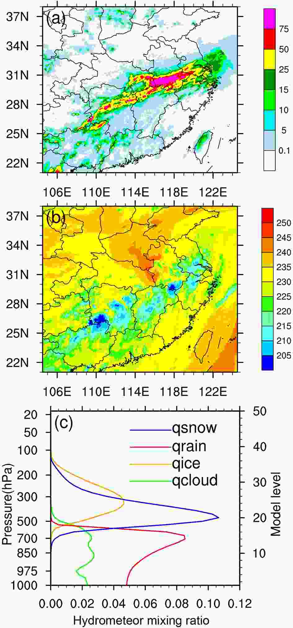
Figure 1. (a) Observed 12-h accumulated precipitation (units: mm) from 0600 UTC to 1800 UTC 2 July 2016 in the study domain, (b) the brightness temperature (K) of channel 8 from Himawari-8 AHI valid at 1800 UTC 2 July 2016, and (c) the vertical profiles of qc, qi, qr, and qs (g kg−1) from one ensemble member valid at 1800 UTC 2 July 2016.
The Weather Research and Forecasting (WRF) model V3.8.1 (Skamarock et al., 2008) is used as the NWP model in this study. The horizontal grid spacing is 4 km, and the number of horizontal grid points is 550×450. The number of vertical levels is 51, and the model top set to 10 hPa. The following physics parameterization schemes are adopted: the WRF single-moment 6-class microphysics scheme (WSM6); the Rapid Radiative Transfer Model for GCMs (RRTMG) shortwave and longwave radiation schemes; the Mellor-Yamada-Janjić (MYJ) boundary layer scheme. No cumulus parameterization is employed.
Considering that hydrometeors evolve rapidly with time, in this study we chose to use the ensemble sample to calculate hydrometeor background errors, as employed in previous studies (Michel et al., 2011; Legrand et al., 2016). In order to obtain the statistical samples of background errors for hydrometeors, an 80-member ensemble forecast was carried out, which was initialized from an 80-member ensemble analysis valid at 0600 UTC 2 July 2016. The 80-member ensemble analysis was provided by the EnKF system of NCEP’s operational Global Data Assimilation System (GDAS). The 12-h forecasts of the 80-member ensemble valid at 1800 UTC 2 July 2016 were used as the statistical samples, and the background errors of hydrometeors were approximated by the deviations of each ensemble member from the ensemble mean. Figure 1c shows the vertical profiles of
${q_{\rm{c}}}$ ,${q_{\rm{i}}}$ ,${q_{\rm{r}}}$ , and${q_{\rm{s}}}$ from one ensemble member. The liquid hydrometeor mixing ratios (${q_{\rm{c}}}$ and${q_{\rm{r}}}$ ) are confined primarily to levels below 500 hPa, while the ice particle mixing ratios (${q_{\rm{i}}}$ and${q_{\rm{s}}}$ ) are only found in the middle and upper levels between 700 and 150 hPa. The magnitude of the four hydrometeors is about 10−5 kg kg−1, so only the levels at which the mean value of each hydrometeor is greater than 10−6 kg kg−1 are diagnosed in this study.This study aims to find a Gaussian transform method to construct more Gaussian hydrometeor control variables in data assimilation systems. Four experiments are designed, and the details of the four experiments are shown in Table 1. The experiment Origin uses the original hydrometeors as a benchmark. It has been pointed out that the logarithmic transform, like denary logarithmic (Log10), can bring the PDFs of background errors for some variables closer to Gaussian (Errico et al., 2007; Fletcher and Zupanski., 2007), so the experiment Log10 employs the logarithm of hydrometeors as in Michel et al. (2011). The Softmax function is used in experiment Softmax in this study; The newly constructed Quasi-Softmax function is employed in the experiment Q_softmax.
Experiments Hydrometeor control variables Origin ${q_{i,j,k}}$ Log10 $\lg \left(\dfrac{{{q_{i,j,k}}}}{{{q_{\rm{0}}}}}\right);{q_0} = {10^{ - 3}}{\rm{kg}}\;{\rm{k}}{{\rm{g}}^{ - 1}} $ Softmax $\dfrac{{\exp (\beta {q_{i,j,k}})}}{{\displaystyle\sum {\exp (\beta {q_{i,j,k}})} }}$ Q_softmax $\frac{{\exp (\beta {q_{i,j,k}})}}{{\displaystyle\sum\limits_{{{\overline q }_{i,j}} > 0} {\exp (\beta {{\overline q }_{i,j}}){\rm{ - }}\displaystyle\sum\limits_{{q_{i,j,k}} > 0} {\exp (\beta {{\overline q }_{i,j}})} } }},{\overline q _{i,j}} = \dfrac{1}{K}\displaystyle\sum\limits_{k = 1}^K {{q_{i,j,k}}} $ Table 1. Four experiments and their hydrometeor control variables.
-
In order to evaluate the impacts of different transform methods on the spatial distribution of hydrometeors, in this subsection the horizontal and vertical distribution of hydrometeors before and after transformation are studied.
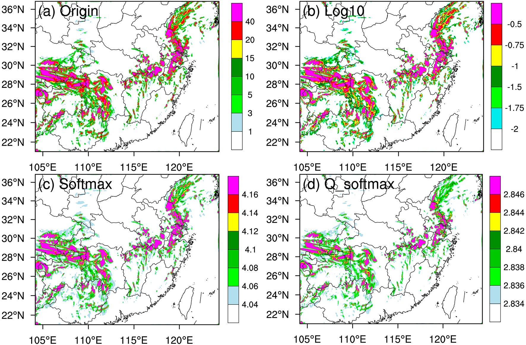
Figure 2 shows the horizontal distribution of the various transformed
${q_{\rm{s}}}$ fields at model level 25 (~300 hPa). The horizontal distribution of${q_{\rm{s}}}$ in the four experiments are similar but display different values, but because all three transform methods are mathematical, this ensures that the values of the variables before and after the transformation can correspond one to one. The values of${q_{\rm{s}}}$ in Log10 has been transformed to be negative ranging from −3 to 0, and the larger the original${q_{\rm{s}}}$ is, the closer to 0 the transformed value in Log10 it will be. Softmax and Q_softmax have similar horizontal distribution characteristics to that of${q_{\rm{s}}}$ , but with different values due to the denominators in the transform function. It is also worth noticing that Softmax and Q_softmax have transformed${q_{\rm{s}}}$ from zero to positive values. Their impact is discussed below.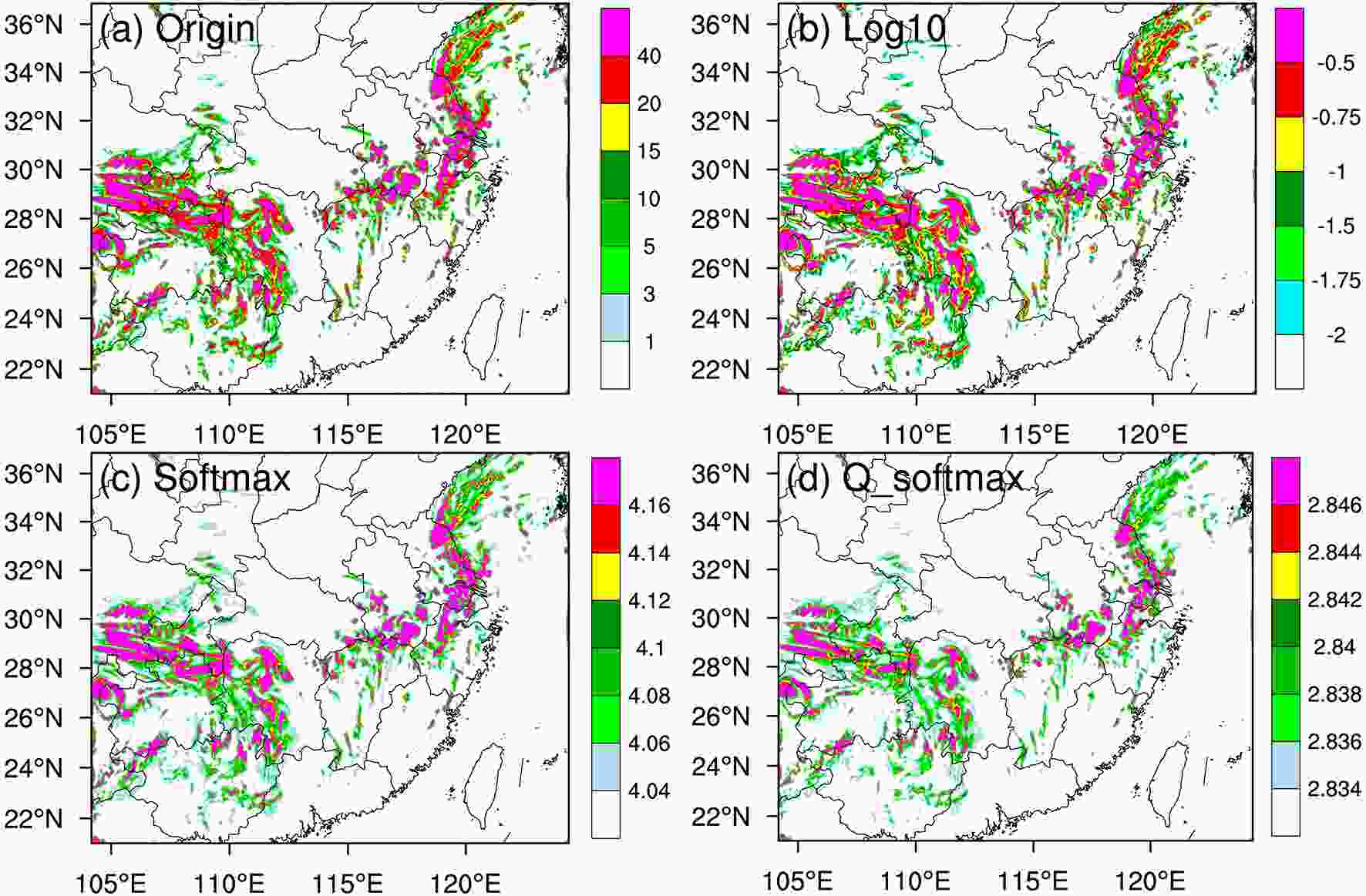
Figure 2. Transformed
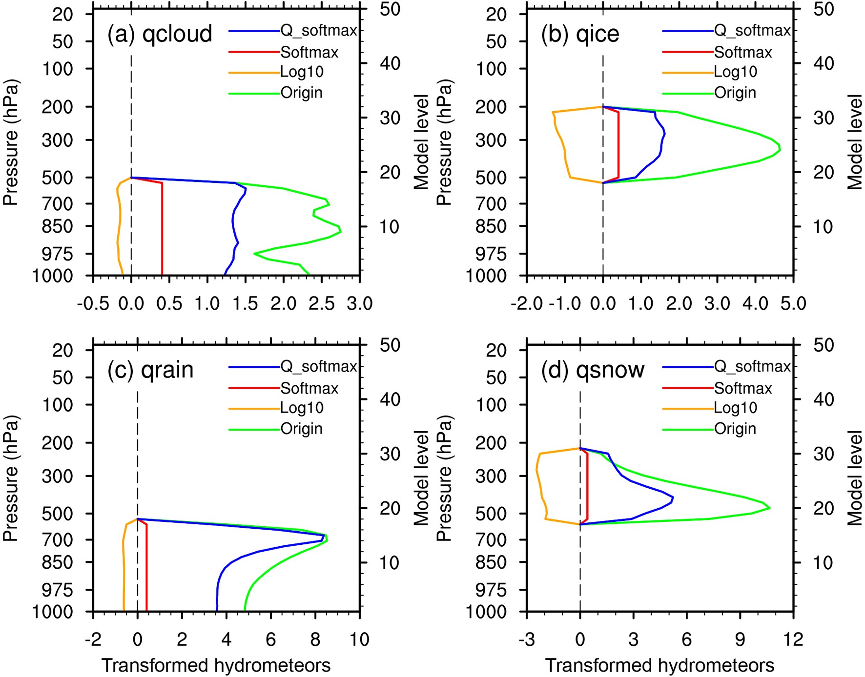
${q_{\rm{s}}}$ at model level 25 (~ 300 hPa) for (a) Origin (10−5 kg kg−1), (b) Log10 (logarithmic transform; kg kg−1), (c) Softmax (10−6 kg kg−1) and (d) Q_softmax (10−5 kg kg−1) from one sample.Compared to the horizontal distribution, the characteristics of the vertical distribution of hydrometeors are greatly changed. Figure 3 shows the vertical profiles of
${q_{\rm{c}}}$ ,${q_{\rm{i}}}$ ,${q_{\rm{r}}}$ , and${q_{\rm{s}}}$ for the four experiments. The vertical distribution of the transformed hydrometeors in Log10 has changed a lot when compared to that in Origin. It can be seen from Fig. 3b that the peaks of the transformed hydrometeors in Log10 are at the levels where the original hydrometeors are less, while the levels with more hydrometeors in Origin cannot be easily distinguished in Log10. The values of the transformed hydrometeors in Softmax are nearly the same at all levels. This can be explained by the fact that the denominators of the Softmax function, which is the sum over the horizontal domain, are very similar at each level. Compared with Log10 and Softmax, the shape of the vertical profiles of transformed hydrometeors in Quasi-Softmax are much closer to that in Origin, indicating that the vertical distribution characteristics of hydrometeor mixing ratios are kept to some extent after using the Quasi-Softmax transformation, and that our modification to the denominator of Softmax function is reasonable.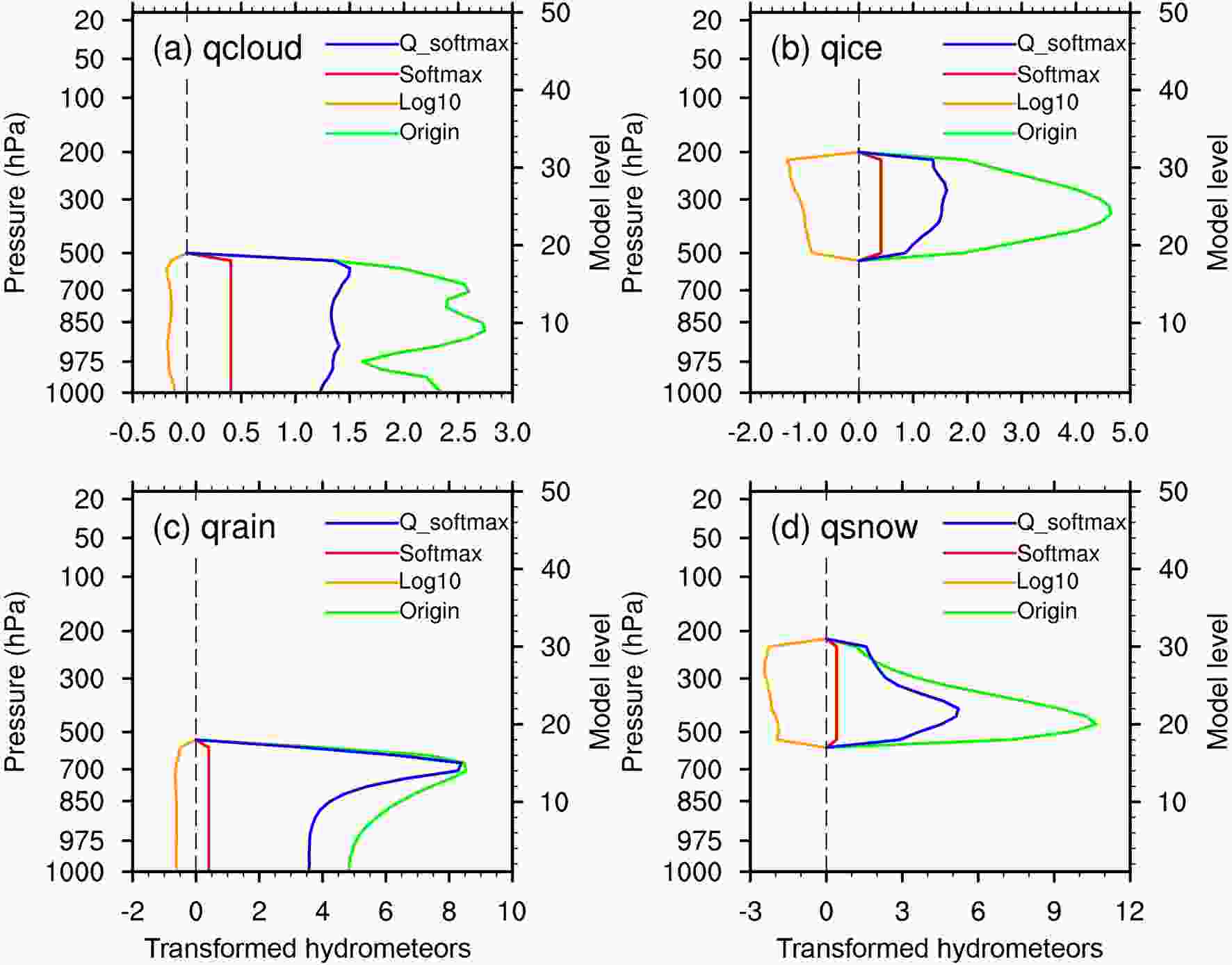
Figure 3. The vertical profiles of (a) qc, (b) qi, (c) qr, and (d) qs for Origin (10−5 kg kg−1), Log10 (kg kg−1), Softmax (10−6 kg kg−1) and Q_softmax (10−5 kg kg−1) from one sample.
-
The spatial distribution of the hydrometeors for the four experiments were compared, and the results show that the characteristics of the distribution of the original hydrometeors are similar with that in the Q_softmax. The NG of the background errors of hydrometeors for different transform methods are further studied in this subsection.
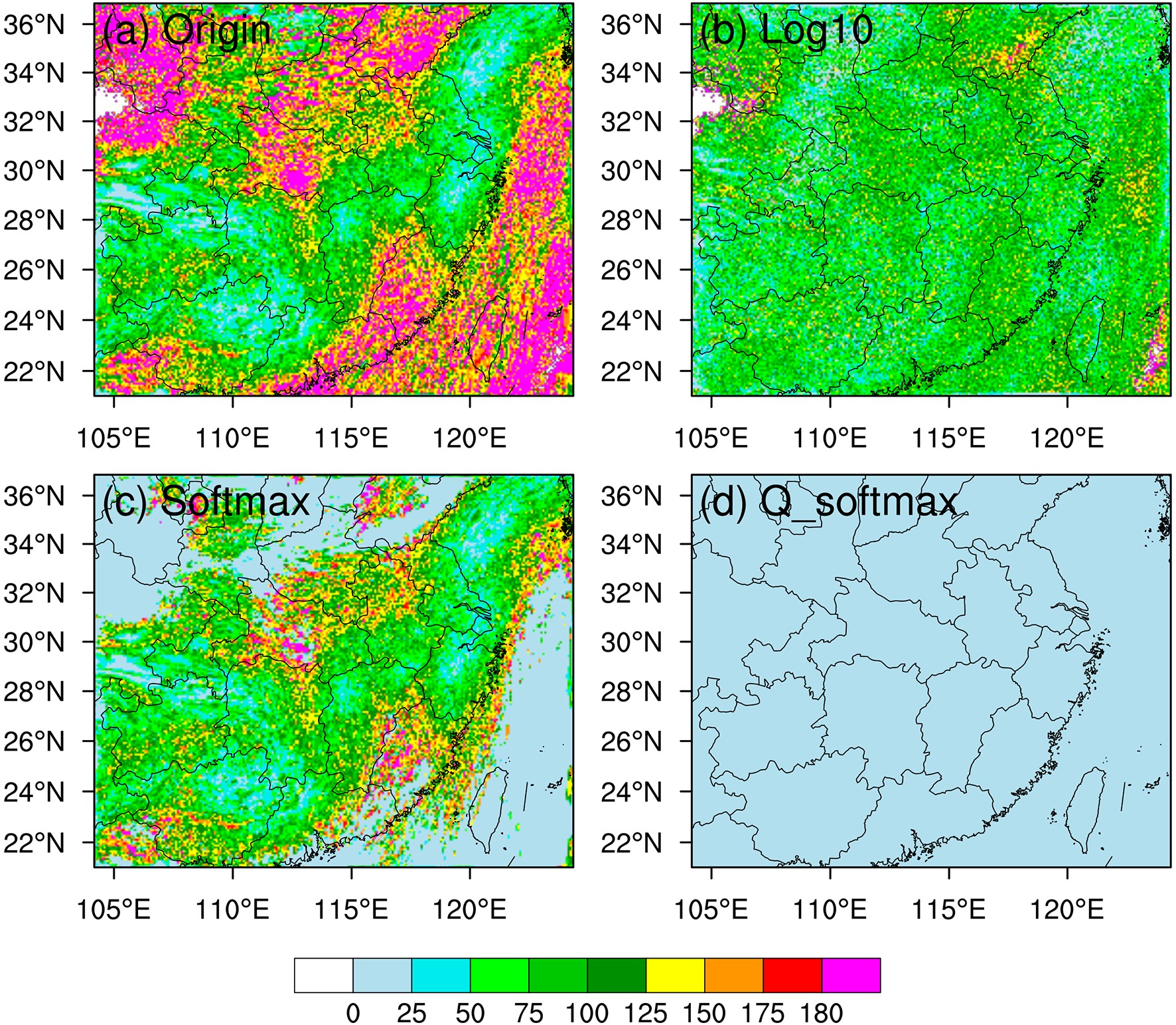
An example of the horizontal structures of NG is given for
${q_{\rm{s}}}$ at the model level 25 (~300 hPa) of the four experiments by Fig. 4. The horizontal K2 values of original${q_{\rm{s}}}$ (Fig. 4a) are large and the maximum value is > 180, indicating high NG of${q_{\rm{s}}}$ . The greatest K2 values in Origin are in the intersections of the clear sky and cloudy regions, while the values are relatively smaller inside the clouds, roughly between 25 and 75. As is shown in Fig. 4b, the NG of the transformed${q_{\rm{s}}}$ in Log10 is decreased in the intersection regions of cloudy and clear sky, but the K2 values in the cloudy regions increase considerably when compared to that in Origin. For the Softmax method (Fig. 4c), the NG in the intersections of cloudy and clear area is reduced much, but the K2 values in cloudy regions are nearly unchanged. Almost all K2 values in Q_softmax (Fig. 4d) have been decreased to < 25, indicating that the${q_{\rm{s}}}$ has been transformed into a more Gaussian-like variable.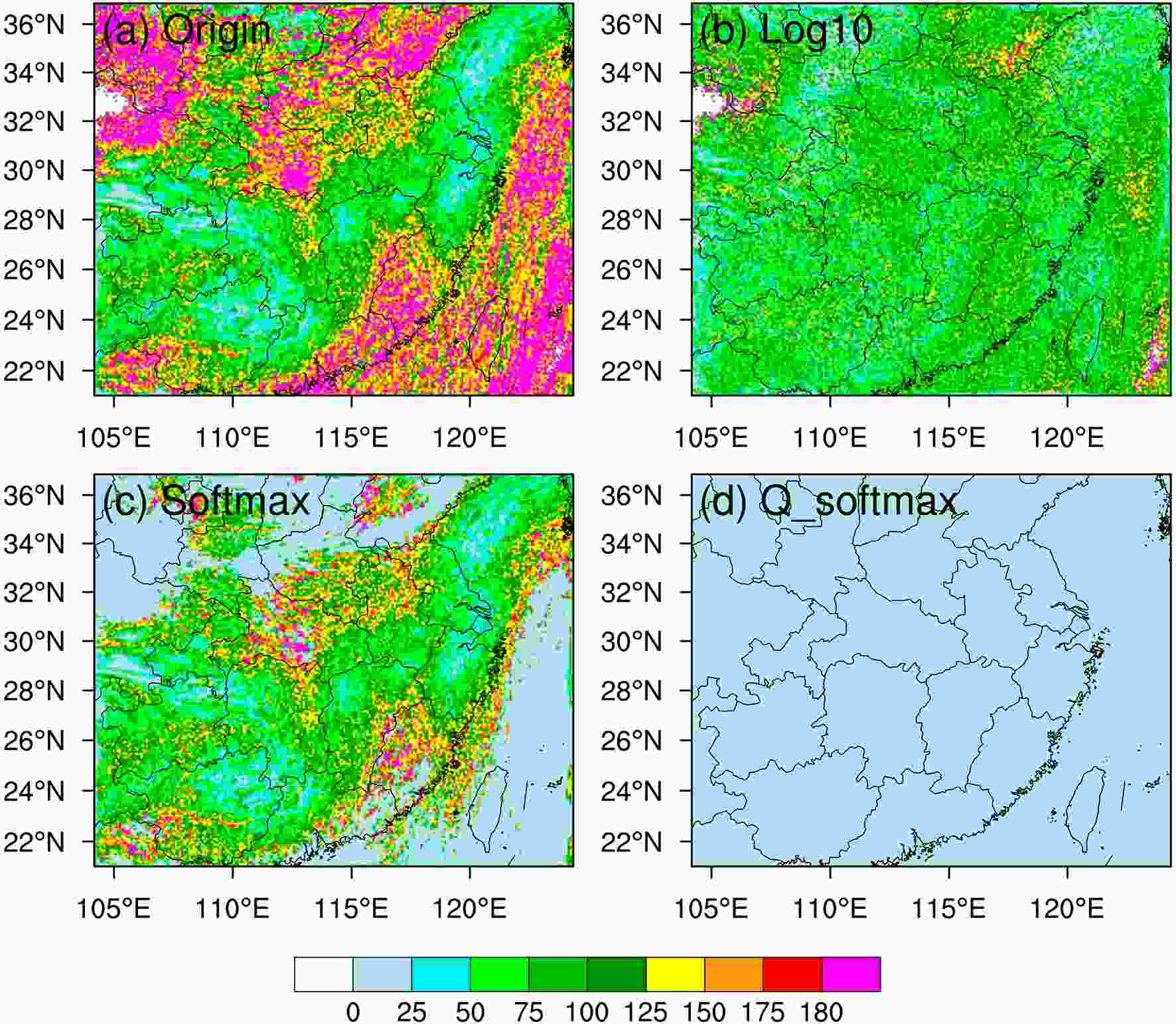
Figure 4. K2 of qs at model level 25 (~ 300 hPa) for (a) Origin, (b) Log10, (c) Softmax and (d) Q_Softmax.
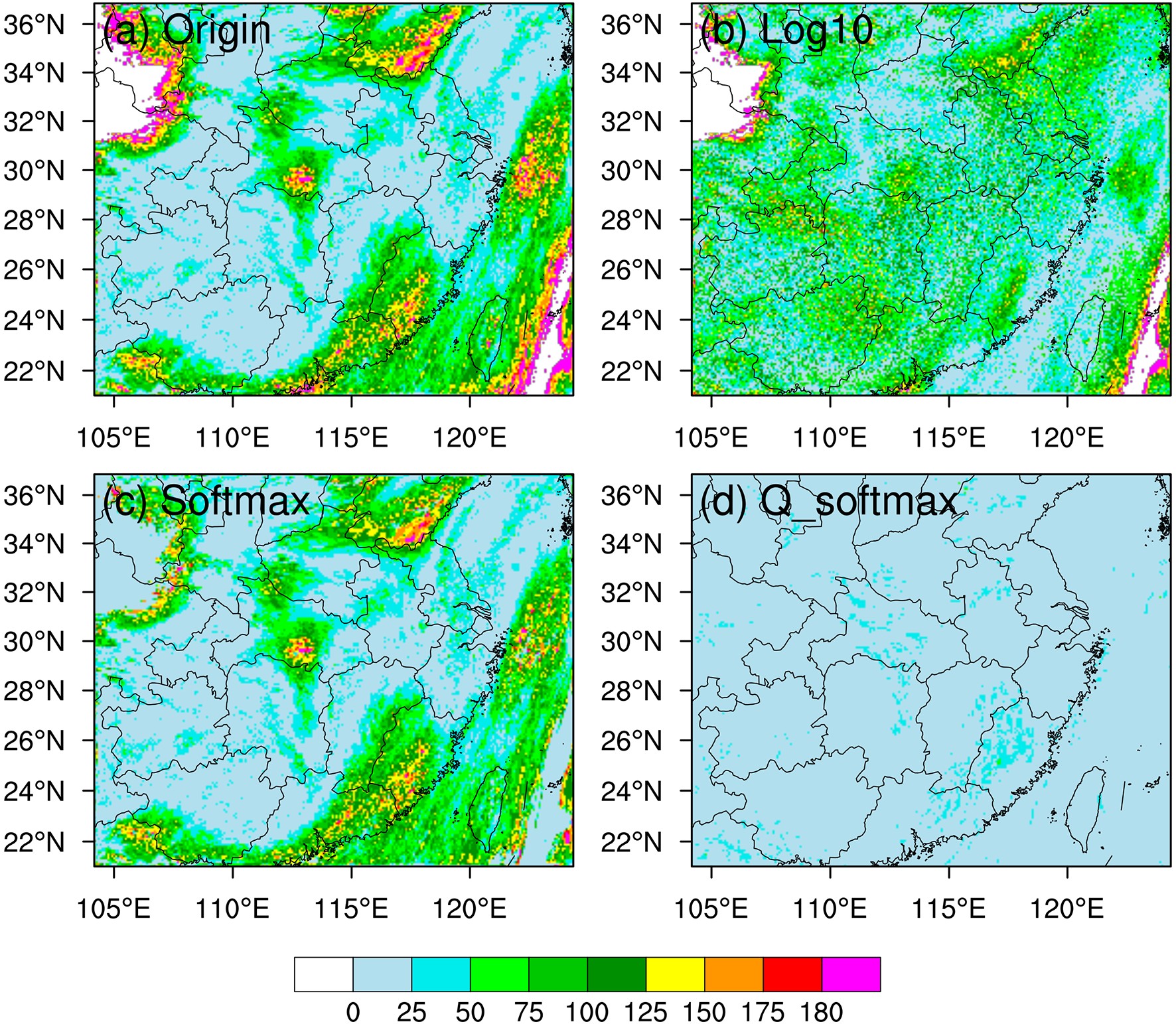
The horizontal distribution of K2 for
${q_{\rm{i}}}$ at model level 25 (~300 hPa) is shown in Fig. 5. In Origin, the NG of${q_{\rm{i}}}$ is decreased considerably when compared to${q_{\rm{s}}}$ , but the NG is still large in the intersection of clear and cloudy regions. Similar with${q_{\rm{s}}}$ , the NG of${q_{\rm{i}}}$ is not decreased either in Log10 or Softmax. However, after transformed by the Q_softmax method, the K2 of${q_{\rm{i}}}$ in most regions are decreased to < 25, indicating the NG has been decreased appreciably. It is also worth noticing that, in the area where there are small K2 values in either Origin and Log10, the K2 values in both Softmax and Q_Softmax are not null. This can be explained by the differences in transforming zero-value quantities among different ensembles, as mentioned previously. To avoid this phenomenon, an effective solution is to calculate the background error covariance in cloudy and clear regions as in Montmerle and Berre (2010), though this is beyond discussion in this study.
Figure 5. K2 of qi at model level 25 (~ 300 hPa) for (a) Origin, (b) Log10, (c) Softmax and (d) Q_softmax.
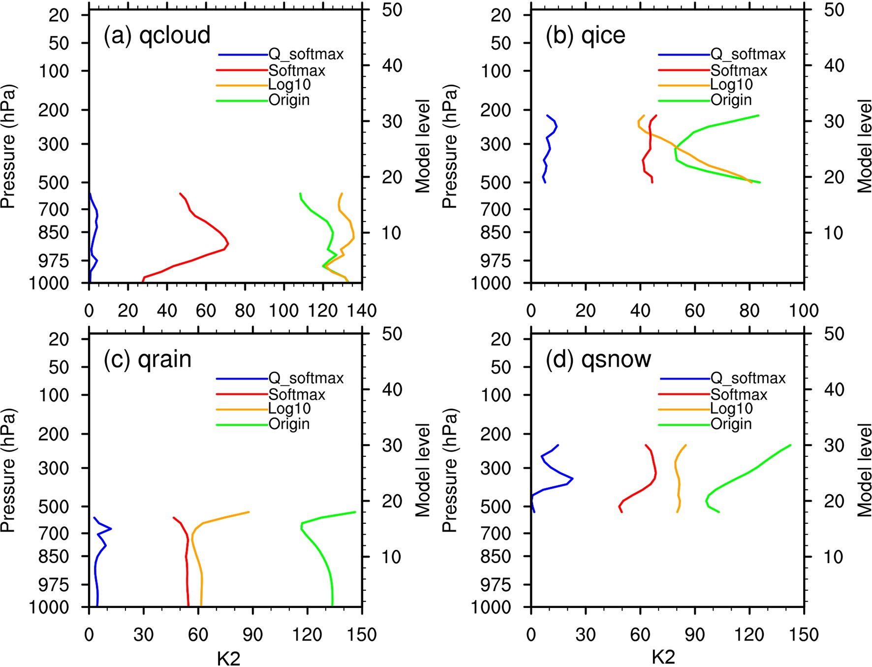
The vertical profiles of K2 for the four experiments related to NG are shown in Fig. 6 for
${q_{\rm{c}}}$ ,${q_{\rm{i}}}$ ,${q_{\rm{r}}}$ , and${q_{\rm{s}}}$ . The original hydrometeors show large deviation from being Gaussian with K2 values > 80 at almost every level. Among the four hydrometeors in Origin,${q_{\rm{i}}}$ is the most Gaussian-like variable since the K2 values range from 50 to 80, though still indicating great NG. Those levels with less hydrometeors have greater NG while the levels with more hydrometeors are relatively more Gaussian-like, indicating that the NG of hydrometeors may be related to the distribution of hydrometeors themselves. The Log10 method slightly decreases the NG of${q_{\rm{r}}}$ ,${q_{\rm{s}}}$ , and${q_{\rm{i}}}$ above 300 hPa, but it increases the NG of${q_{\rm{c}}}$ , and${q_{\rm{i}}}$ below 300 hPa, meaning that the logarithm of hydrometeors still has great NG. When compared to Origin and Log10, the NG of the transformed hydrometeors is decreased considerably in Softmax, except for${q_{\rm{c}}}$ near 975 hPa and${q_{\rm{i}}}$ above 250 hPa. The K2 values are decreased to < 60 in Softmax for the four hydrometeors, but it is still far from being Gaussian. The Quasi-Softmax method shows the most promising results in that the K2 values of all hydrometeors at almost every level are reduced to < 10, meaning that the hydrometeors have been transformed into more Gaussian-like variables. Even though the K2 values of${q_{\rm{s}}}$ near 200 hPa and 400 hPa are a little larger, it still outperforms the other three methods. The results show that, with the Quasi-Softmax transform, the hydrometeors can be transformed into more Gaussian-like variables, which therefore can act as the hydrometeor control variable candidates in data assimilation systems.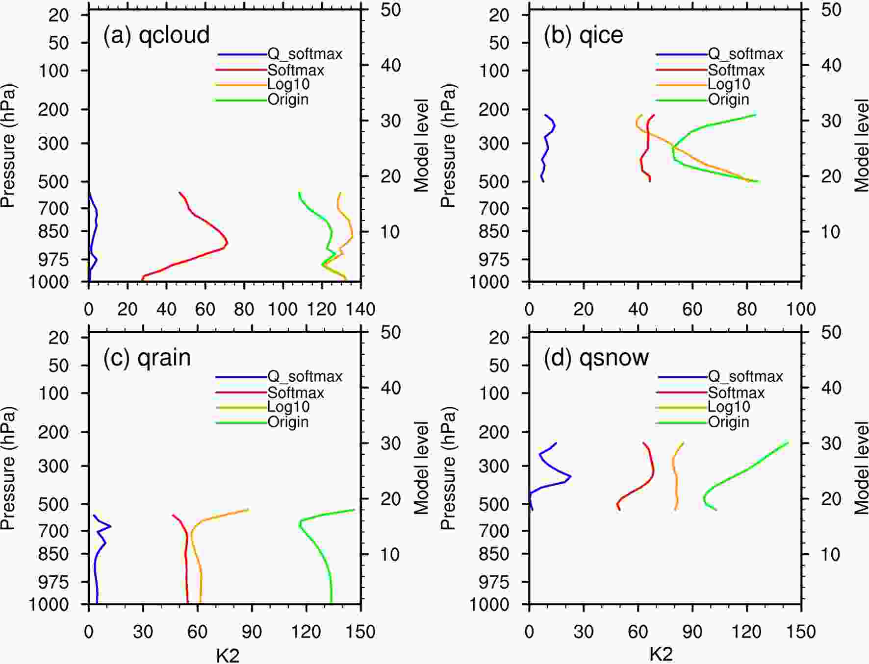
Figure 6. Vertical profiles of K2 of (a) qc, (b) qi, (c) qr, and (d) qs for the four experiments. For each level, values are averaged over the horizontal domain.
-
In the previous two subsections, the spatial distribution characteristics and NG of the background errors of the hydrometeors for the four experiments were discussed. It was shown that the transformed hydrometeors in Q_Softmax exhibit a reasonable spatial distribution and are the most Gaussian variables among the four experiments. In this subsection, the background error characteristics of hydrometeors for the four experiments are discussed to further evaluate whether the background errors of the transformed hydrometeors are reasonable. The horizontal, vertical variances and the horizontal length scale are discussed, respectively.
In the data assimilation, the weight of observations to analysis depends on the relative size of the background errors and the observation errors, so the variance of background errors plays a vital role in the data assimilation. Figure 7 shows the horizontal standard deviation (SD) of
${q_{\rm{s}}}$ at the model level 25 for the four experiments. As is shown in Fig. 7a, the SD of the original hydrometeors are larger in the cloudy regions (Fig. 2b) than that in the clear area, indicating that the uncertainties are greater in cloudy regions. The situation reverses for the experiment Log10 (fig. 7b), where larger SD exists in the clear air while being relatively smaller in cloudy regions. This may be explained by the fact that zero-values were not transformed in Log10 in some members, thus the contrast among the 80 members was increased after transformation. For experiments Softmax and Q_softmax, the characteristics of the horizontal distribution of SD are similar with that in Origin, but the values are relatively smaller.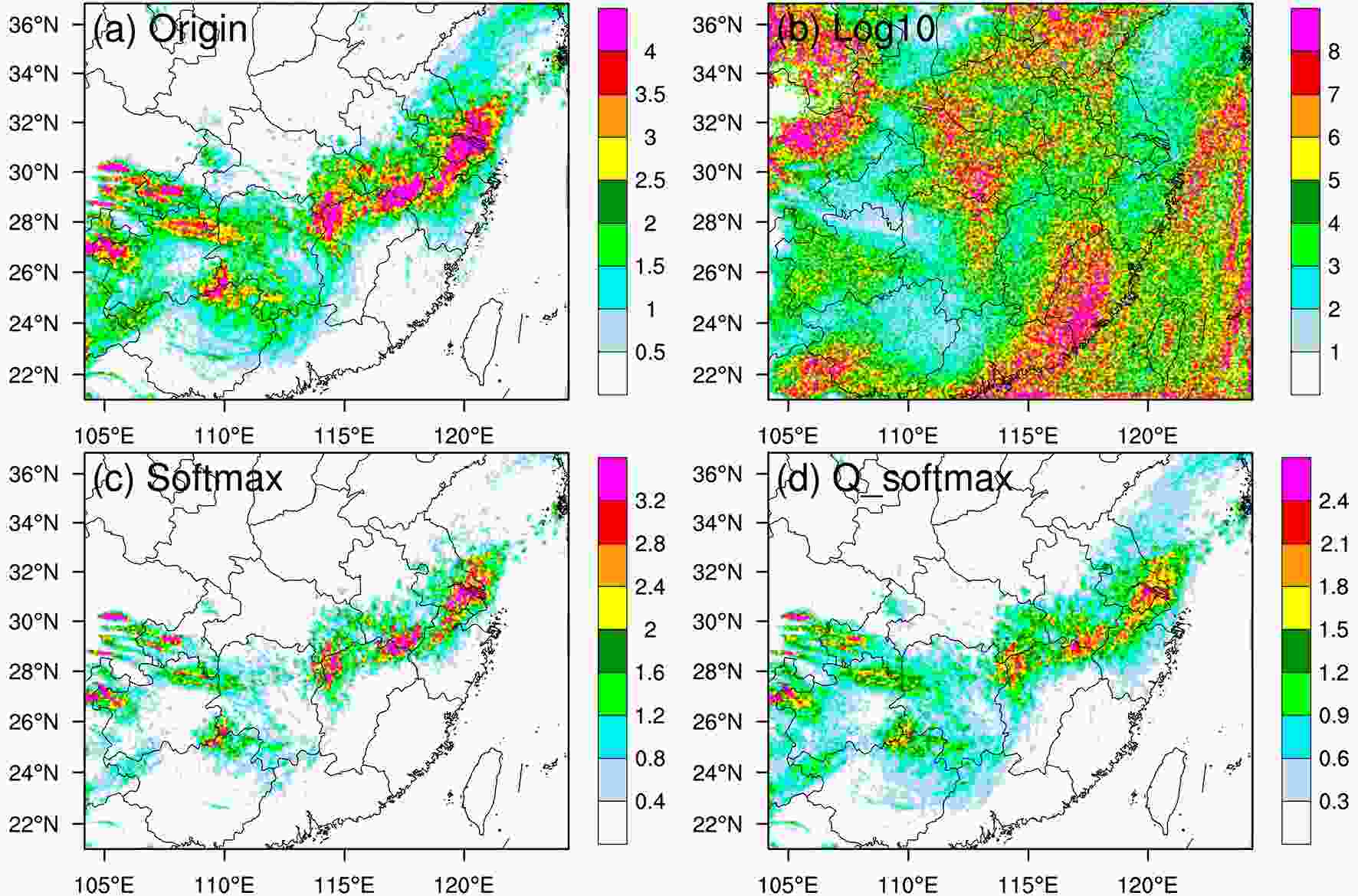
Figure 7. Horizontal standard deviation of the transformed qs at the 25th model level for (a) Origin (10−4 kg kg−1), (b) Log10 (kg kg−1), (c) Softmax (10−7 kg kg−1) and (d) Q_Softmax (10−6 kg kg−1).
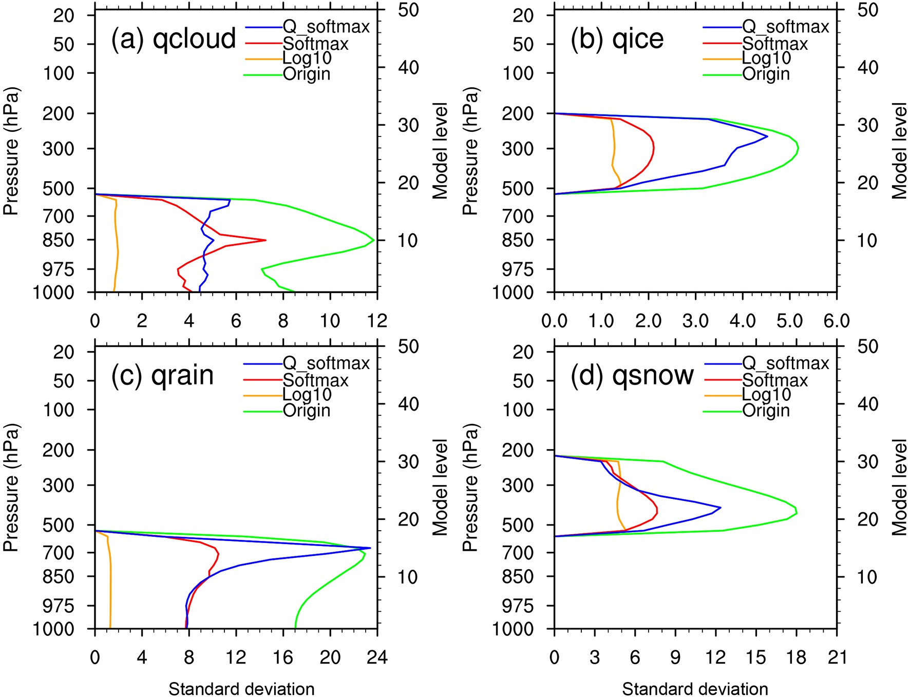
Figure 8 shows the vertical profiles of the SD of the hydrometeors for the four experiments. For the original hydrometeor mixing ratios, the vertical distribution of SD is similar to the vertical distribution of hydrometeors themselves. The SD is larger at the levels where the hydrometeors are greater, which means that the uncertainty of hydrometeors are larger at these levels. The values of the SD of the experiment Log10 are almost the same at all levels for the four hydrometeors, though this may not properly represent the vertical characteristics of the background errors of hydrometeors. The vertical characteristics of SD in Softmax is similar to that in Origin. The vertical profile of SD for hydrometeors in Quasi-Softmax is also close to that in Origin except for
${q_{\rm{c}}}$ between 700 hPa and 500 hPa and${q_{\rm{r}}}$ near 600 hPa. Generally, the hydrometeors transformed by the Quasi-Softmax function reasonably represent the vertical characteristics of background errors for hydrometeors. It is noted that the vertical structures are relatively sharper in Q_softmax, which may be not good for BE modeling. This may be explained by the large differences in denominators of the Quasi-Softmax function in different levels. To handle this problem, one potential solution is to introduce a vertical smoother in Quasi-Softmax function, such as averaging the denominators in Quasi-Softmax function of current level with its near upper and lower levels.
Figure 8. Vertical standard deviation profile of (a) qc, (b) qi, (c) qr, and (d) qs for Origin (10−5 kg kg−1), Log10 (10 kg kg−1), Softmax (10−8 kg kg−1) and Q_softmax (10−7 kg kg−1).
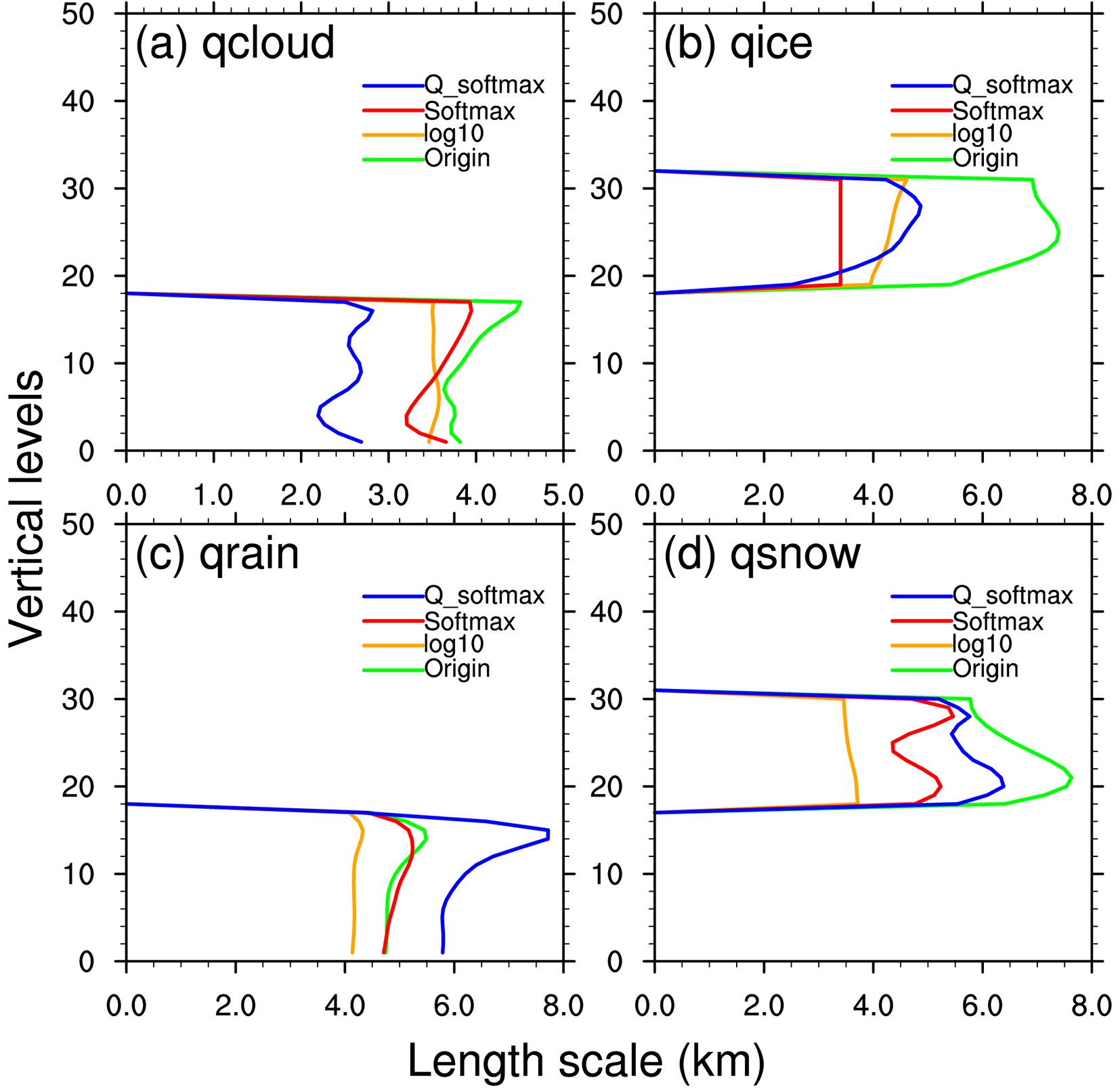
The horizontal length scale is an important parameter which determines how far the observations can be spread in the control variable space. Figure 9 shows the horizontal length scales of the four hydrometeors for the four experiments. The length scales of the original hydrometeors are all < 8 km (2 model grid lengths), which means that the observations containing hydrometeor information will spread a much shorter distance when compared to the common control variables like wind, temperature, and humidity. For
${q_{\rm{c}}}$ , the length scales for the four experiments at all levels are less than 5 km, with the scale in Origin being the largest. The structures of the length scale in Softmax and Q_softmax are similar to that in Origin. For${q_{\rm{i}}}$ , the length scale in Origin is nearly 8 km, while the characteristics of length scale in Q_Softmax method is the closest to that in Origin. The length scale of${q_{\rm{i}}}$ in Softmax is very close at each level, which may be explained by the fact that the spatial correlation of transformed${q_{\rm{i}}}$ is very similar using the Softmax transform method. When it comes to${q_{\rm{r}}}$ , the length scales in Softmax closely approximate those in the Origin method, and the shape in Q-softmax is similar to those two but with relatively larger length scales. The length scales of${q_{\rm{s}}}$ in Q_Softmax are similar to that in Origin except for the levels near model level 28. Considering that the length scales of hydrometeors are relatively smaller, the differences among the four experiments can be neglected when they are applied to the data assimilation systems.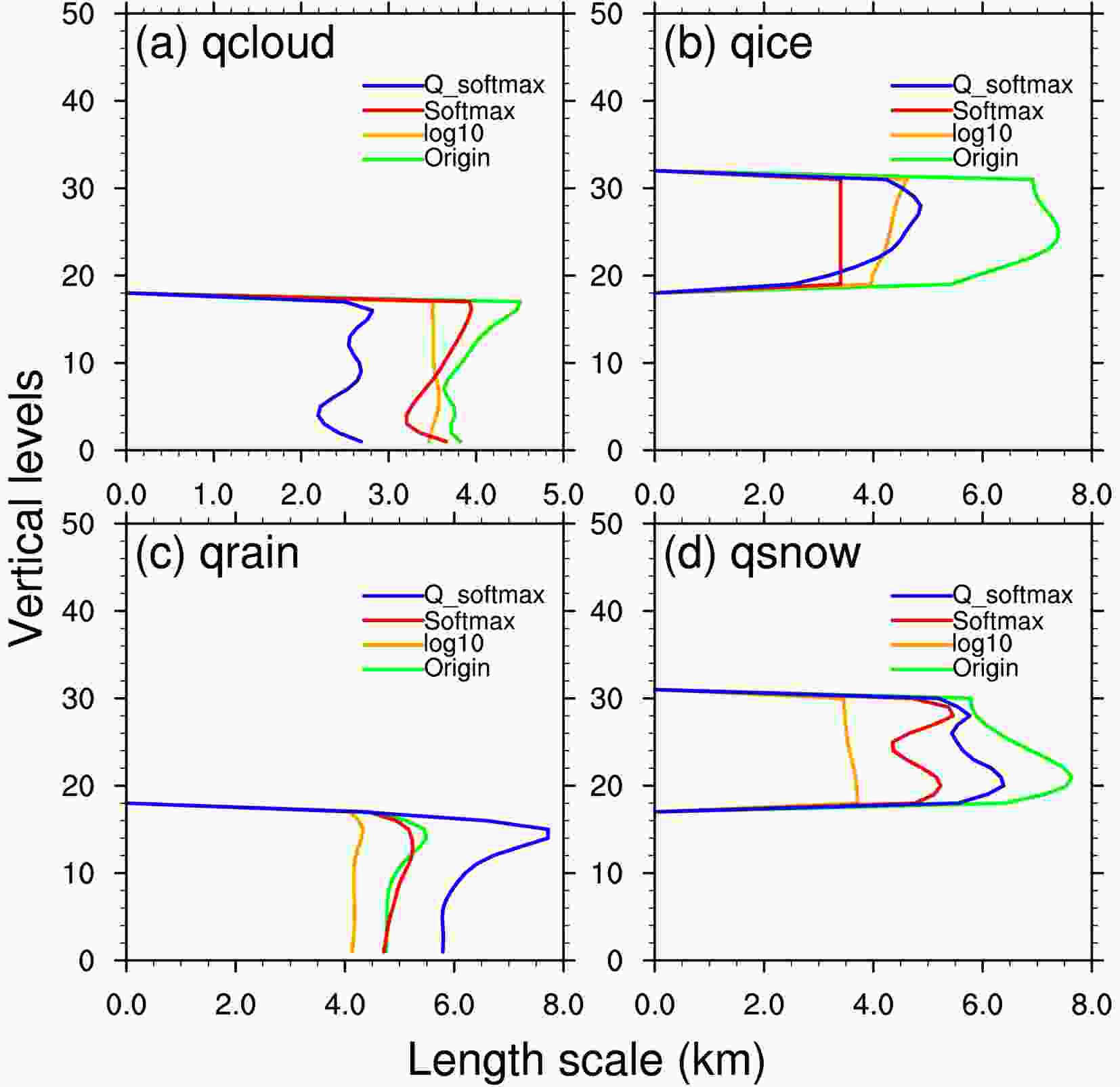
Figure 9. Horizontal length scale (km) for (a) qc, (b) qi, (c) qr, and (d) qs for Origin, Log10, Softmax and Q_softmax.
-
A new Gaussian transform method, Qusai-Softmax transform, was proposed to construct more Gaussian hydrometeor control variables satisfying the Gaussian unbiased assumptions of the data assimilation systems. The new Gaussian transform method was compared with the other three transform methods from the perspectives of the spatial distribution, the NG of background errors and the characteristics of background error covariances. A precipitation case from the rainy season of China was selected and an 80-member ensemble of 12-h forecasts was generated to obtain statistical samples of the background errors of hydrometeors.
Firstly, the horizontal and vertical distribution characteristics of hydrometeors for the four different transform methods were discussed. The characteristics of the horizontal distribution characteristics of original hydrometeor mixing ratios were kept in experiments Log10, Softmax and Q_softmax, but the vertical distribution characteristics varied a lot in these three experiments. The Log10 and Softmax methods changed the vertical distribution greatly, while the Quasi-Softmax method basically kept the characteristics of vertical structures of hydrometeors.
The D′Agostino test was used to diagnose the NG of background errors of the transformed hydrometeors. The original hydrometeors showed great NG, especially in the intersection areas between cloudy and clear regions, where the greatest uncertainty occurred. The Log10 method slightly improves the NG in the intersection areas but increased the NG in cloudy areas. The Softmax method improved the NG considerably in the intersection areas between cloudy and clear regions, but did not help in the cloudy area. The Quasi-Softmax decreased the NG of hydrometeors significantly and the transformed hydrometeors were much closer to a Gaussian distribution. The Softmax and Quasi-Softmax methods produced a new problem that the hydrometeors in clear areas are transformed such as not to have null values, indicating that the transformation should not be carried out in clear areas. These and other issues should be taken into consideration and will be explored in future work.
The new Gaussian transform was added to the CVTs of the background error covariances, and the characteristics of
${{B}}$ for different transformed hydrometeors were compared. The Log10 method greatly changed the variance distribution both vertically and horizontally, while the characteristics of the variances of transformed hydrometeors using the Softmax and Quasi-Softmax methods showed reasonable results both in the horizontal and vertical variances. The horizontal length-scales for the three transformed hydrometeor types were all reduced when compared to original hydrometeor mixing ratios. The horizontal length-scales only covered < 2 model grid-lengths, so the differences among those transformed methods make little sense by tuning the length scales.In this study, the new Gaussian transform method was only evaluated by measuring the NG of the transformed hydrometeors and diagnosing the characteristics of the background errors. The new Gaussian transform method will be implemented to the data assimilation system, and its application to the assimilation of radar reflectivity or satellite radiance retrievals will be studied further in the near future. We also noticed that some Gaussian transform methods have been applied to other fields, like the Gaussian anamorphosis method applied to precipitation variables (Lien et al., 2013; Kotsuki et al., 2017). It is worth exploring application of this method to hydrometeors. Besides, some assimilation techniques based on the non-Gaussian framework, like particle filters, has been developed and applied in the recent decade (Poterjoy, 2016; Buehner and Jacques, 2020; Kawabata and Ueno, 2020), and it is also worth exploring their handling of NG in the assimilation of cloud-sensitive observations at convective scales.
Acknowledgements. This research was funded by National Key Research and Development Program of China (Grant No. 2017YFC1502102), National Natural Science Foundation of China (Grant No. 42075148), and Graduate Research and Innovation Projects of Jiangsu Province (Grant No. KYCX20_0910). The numerical calculations of this study are supported by the High-Performance Computing Center of Nanjing University of Information Science and Technology (NUIST).
| Experiments | Hydrometeor control variables |
| Origin | ${q_{i,j,k}}$ |
| Log10 | $\lg \left(\dfrac{{{q_{i,j,k}}}}{{{q_{\rm{0}}}}}\right);{q_0} = {10^{ - 3}}{\rm{kg}}\;{\rm{k}}{{\rm{g}}^{ - 1}} $ |
| Softmax | $\dfrac{{\exp (\beta {q_{i,j,k}})}}{{\displaystyle\sum {\exp (\beta {q_{i,j,k}})} }}$ |
| Q_softmax | $\frac{{\exp (\beta {q_{i,j,k}})}}{{\displaystyle\sum\limits_{{{\overline q }_{i,j}} > 0} {\exp (\beta {{\overline q }_{i,j}}){\rm{ - }}\displaystyle\sum\limits_{{q_{i,j,k}} > 0} {\exp (\beta {{\overline q }_{i,j}})} } }},{\overline q _{i,j}} = \dfrac{1}{K}\displaystyle\sum\limits_{k = 1}^K {{q_{i,j,k}}} $ |


 AAS Website
 AAS WeChat