


 DownLoad:


-
Database profile Database title CAS FGOALS-f3-L Model Datasets for CMIP6 DCPP Experiment Time range dcppA-hindcast: 1960–2016
dcppB-forecast: 2017–21Geographical scope dcppA-hindcast: global
dcppB-forecast: globalData format version 4 of Network Common Data Form (NetCDF) Data volume 4.07 TB for dcppA-hindcast
351GB for dcppB-forecastData service system https://esg.lasg.ac.cn/CMIP6/DCPP/CAS/FGOALS-f3-L/ Sources of funding The National Key Research and Development Program of China (Grant No. 2018YFA0606300), the NSFC (Grant No. 42075163), the NSFC BSCTPES project (Grant No. 41988101), and the NSFC (Grant No. 42205039) Database composition 1. The dcppA-hindcast comprises nine-member hindcasts initialized on 25, 28, and 30 November for each year during 1960–2016, containing 44 monthly mean atmospheric and oceanic variables.2. The dcppB-hindcast comprises nine-member hindcasts initialized on 25, 28, and 30 November for each year during 2017–21, containing 44 monthly mean atmospheric and oceanic variables. -
Decision-making processes for climate change adaptation and mitigation rely heavily on climate change information for the next 10 years, which is estimated by using decadal climate prediction (also referred to as near-term climate prediction). Decadal climate prediction lies between seasonal to interannual prediction and long-term climate projection, serving as an indispensable part of seamless climate prediction (Meehl et al., 2021).
As a topic on the international scientific frontier, decadal climate prediction has become a hotspot in climate change research over the last decade. Since 2007, many climate modeling centers around the world have been actively developing decadal prediction systems and conducting decadal prediction experiments (Kataoka et al., 2020; Bethke et al., 2021; Bilbao et al., 2021; Sospedra-Alfonso et al., 2021; Carmo-Costa et al., 2022). The World Climate Research Program (WCRP) has identified decadal climate prediction as one of seven grand challenges (Kushnir et al., 2019) and listed “Prediction of the near-term evolution of the climate system” as one of four scientific objectives of the WCRP Strategic Plan 2019–2028 (WCRP JSC, 2019). The decadal climate prediction experiment was one of two core experiments of the Coupled Model Intercomparison Project Phase 5 (CMIP5) (Taylor et al., 2009). The Decadal Climate Prediction Project (DCPP) was further endorsed by the Coupled Model Intercomparison Project Phase 6 (CMIP6) (Boer et al., 2016).
Decadal climate prediction is essentially a combination of the initial value problem and the forced boundary value problem (Meehl et al., 2009). There are three sources of climate predictability at decadal to interdecadal time scales, including the committed change (caused by the inertia of the oceans as a response to historical external forcing), the time evolution of internally generated climate variability, and the future path of external forcing (Kirtman et al., 2013). The major difference between decadal prediction and climate projection is that the former’s model initial states are obtained through initialization, that is, assimilating observational data into the model. The specified external forcing for decadal predictions is identical to the non-initialized climate simulations (Doblas-Reyes et al., 2013).
Remarkable progress has been made in assessments of decadal predictions (Smith et al., 2020). The multi-year averaged global mean surface temperature and sea surface temperature (SST) in the North Atlantic (Borchert et al., 2021), the tropical Indian Ocean (Guemas et al., 2013), the Southern Ocean (Saurral et al., 2020), and the North Pacific (Meehl et al., 2016) are highly predictable. However, the decadal prediction skill for land precipitation is generally lower, except for some scattered areas such as the Sahel, the Tibetan Plateau, and Northeast Eurasia (Sheen et al., 2017; Smith et al., 2019; Hu and Zhou, 2021).
The DCPP is a coordinated multi-model investigation into decadal prediction, predictability, and variability that contributes to CMIP6, to the World Climate Research Programme (WCRP) Grand Challenge on Near Term Climate Prediction, and to other activities (https://www.wcrp-climate.org/dcp-overview) (Boer et al., 2016). Component A includes the assimilation experiments and the retrospective decadal forecasts (hindcasts) experiments. The assimilation experiments introduce observation-based data into the model through data assimilation methods to generate initial conditions for hindcasts/forecasts. The hindcasts are integrated for up to several years and used to measure the predictive skill and predictability of historical climate variations. Component B undertakes the quasi-real-time decadal forecasts as a basis for potential operational forecast production. Component C includes several slice experiments of decadal prediction for either natural or naturally forced climate variations (e.g., the global warming hiatus and volcanoes), which are used to support the mechanism studies of decadal prediction.
The Flexible Global Ocean–Atmosphere–Land System (FGOALS-f3-L) climate system model is a fully coupled general circulation model developed by the State Key Laboratory of Numerical Modeling for Atmospheric Sciences and Geophysical Fluid Dynamics (LASG) in the Institute of Atmospheric Physics (IAP) of the Chinese Academy of Sciences (CAS) (Guo et al., 2020a, b; He et al., 2020). We have recently finished the DCPP decadal hindcast (Component A) and decadal forecast (Component B) simulations. In this paper, we provide descriptions of the experiment designs and data outputs.
The remainder of this paper is organized as follows. The model, experimental designs and validation methods are introduced in section 2. In section 3, we show the preliminary technical validation of the outputs from the CAS FGOALS-f3-L decadal prediction experiments. In section 4, usage notes are provided.
-
The FGOALS-f3-L model is one of three versions of CAS models that have participated in CMIP6 [see (Zhou et al., 2020) for a review of Chinese contributions to CMIP6]. It is the low-resolution version of FGOALS-f3, labelled by “L”. Its atmospheric component is version 2.2 of the Finite-volume Atmospheric model (FAMIL) (Zhou et al., 2012; Bao et al., 2019; Li et al., 2019), with a horizonal resolution approximately equal to 1°×1°. The FAMIL has 32 layers in the vertical direction, with the top layer at 2.16 hPa (Guo et al., 2020a; He et al., 2020). The “f” in FGOALS-f3-L represents the atmospheric component FAMIL. Its ocean component is the low-resolution version 3 of the LASG/IAP Climate system Ocean Model (LICOM3) (Liu et al., 2012; Yu et al., 2018; Lin et al., 2020), with a horizontal resolution of 1°×1°. To better resolve equatorial waves, the meridional resolution refines from 1° to 0.5° near the equator. The low-resolution LICOM3 has 30 layers in the vertical direction, which has 10-m layers in the upper 150 m and uneven vertical layers below 150 m. Its land and sea ice components are version 4.0 of the Community Land Model (CLM4) (Oleson et al., 2010) and version 4 of the Los Alamos sea ice model (CICE4) (Hunke and Lipscomb, 2010), respectively. These four components are coupled together through version 7 of the coupler module from the National Center for Atmospheric Research (NCAR) (
http://www.cesm.ucar.edu/models/cesm1.0/cpl7/ ).More details of the basic framework configuration and simulation performance of CAS FGOALS-f3-L can be found in He et al. (2019, 2020), and Guo et al. (2020a).
-
The FGOALS-f3-L was initialized through the upgraded weakly coupled data initialization scheme EnOI-IAU (Wu et al., 2018). The EnOI-IAU initialization scheme integrates two conventional assimilation approaches, ensemble optimal interpolation (EnOI) and incremental analysis update (IAU). The EnOI generates analysis increments (Oke et al., 2002), and the IAU incorporates the increments into the model (Bloom et al., 1996). The EnOI does not need ensemble simulations because its background error covariance is fixed and pre-prepared, which greatly reduces computational cost. In this study, the background error covariance matrix is derived from the historical simulations.
The EnOI-IAU scheme was developed from the IAU scheme that assimilates gridded oceanic analysis data (Wu and Zhou, 2012; Wu et al., 2015). The EnOI-IAU has been used for the FGOALS-s2 models and has shown high skill for interannual and interdecadal predictions (Sun et al., 2018; Wu et al., 2018; Hu et al., 2019, 2020). Compared with that applied to the FGOALS-s2, the EnOI-IAU scheme is upgraded for the new decadal prediction experiment in the following three aspects. First, horizontal localization is introduced, that is, the model-state variables are not influenced by observations farther than the distance of the localization radius (Anderson, 2007). The localization radius is set as
$ 2000\;\mathrm{ }\mathrm{ }\mathrm{ }\mathrm{ }\mathrm{k}\mathrm{m}\times \mathrm{c}\mathrm{o}\mathrm{s}\left(\mathrm{l}\mathrm{a}\mathrm{t}\mathrm{i}\mathrm{t}\mathrm{u}\mathrm{d}\mathrm{e}\right) $ in this study. Second, global observations are assimilated with non-assimilation zones in the high latitudes being removed, which would eliminate artificial discontinuity between assimilation and non-assimilation zones. Third, the number of fixed ensemble members for calculating the background error covariance in the EnOI is increased from 100 to 150, which can generate more accurately sampled covariances.The assimilation acted only on the ocean component of the coupled model. The other model components are controlled by the ocean component through the model coupling processes. The assimilated observational datasets include: (1) gridded SST from the HadISST version 1.1, with a resolution of 1.0°×1.0° (Rayner et al., 2003), and (2) upper-level (0–1000-m) temperature and salinity profiles from the EN.4.2.2 dataset produced by the Hadley Centre (Good et al., 2013). The data climatology is removed and replaced by the model climatology before the assimilation, that is, anomaly initialization was performed (Smith et al., 2013). The climatology of the EN4 profiles was estimated using the gridded analysis product of the EN4 for the period of 1961–90. The model climatology was derived from the ensemble mean of the historical runs over the same period.
Based on the EnOI-IAU initialization scheme, we conducted three independent assimilation experiments, named as Assim-as1, Assim-as2, and Assim-as3, respectively. The assimilation runs were conducted from 1950 to the present. The first ten-year results were not used. They each provided initial conditions for three sets of hindcast/forecast experiments.
-
For the DCPP Component A (Component B), nine-member 10-year hindcast (forecasts) experiments were conducted once per year for the period of 1960–2016 (2017–21), with initial conditions derived from the outputs of the three assimilation experiments. For each assimilation run, the outputs on 25, 28, and 30 November were specified as initial conditions for the three hindcast/forecast runs, respectively. During the integrations of the hindcast/forecast runs, time-varying external radiative forcing due to natural factors and anthropogenic activity was specified. The specified forcing before 2014 is the same as the CMIP6 historical climate simulation experiments. For the forecasts after 2014, the “medium” Shared Socioeconomic Pathway (SSP) 2-4.5 forcing of Scenario MIP is used. The experiments conducted in this study are summarized in Table 1.
Experiment_id Variant_label Experimental design dcppA-hindcast r1i1p1f1-r3i1p1f1 Hindcasts initialized on 25, 28, and 30 November for each year during 1960–2016, with initial conditions derived from the Aassim-as1 experiments r4i1p1f1-r6i1p1f1 Hindcasts initialized on 25, 28, and 30 November for each year during 1960–2016, with initial conditions derived from the Aassim-as2 experiments r7i1p1f1-r9i1p1f1 Hindcasts initialized on 25, 28, and 30 November for each year during 1960–2016, with initial conditions derived from the Aassim-as3 experiments dcppB-forecast r1i1p1f1-r3i1p1f1 Forecasts initialized on 25, 28, and 30 November for each year during 2017–21, with initial conditions derived from the Aassim-as1 experiments r4i1p1f1-r6i1p1f1 Forecasts initialized on 25, 28, and 30 November for each year during 2017–21, with initial conditions derived from the Aassim-as2 experiments r7i1p1f1-r9i1p1f1 Forecasts initialized on 25, 28, and 30 November for each year during 2017–21, with initial conditions derived from the Aassim-as3 experiments Table 1. Experiment designs.
-
Lead-time dependent model drifts due to the initial shock were removed from each month of the prediction data to produce anomalies relative to the period 1970 to 2016 for the hindcasts and forecasts in advance, following the procedures recommended by Boer et al. (2016). We used the anomaly correlation coefficient (ACC) and the mean squared skill score (MSSS) to evaluate prediction skill. The predictive targets analyzed in this study are the annual mean variables in the first forecast year (labeled as year-1), averages over the forecast years 1–5 (labeled as year-1-5), and 6–10 (labeled as year-6-10). As an example, the prediction case started from November in 1960, the year 1961 is the target of the year-1 prediction, and the average over 1961–65 (1966–70) is the target of the year-1-5 (year-6-10) prediction.
We use two metrics to measure the predictive skill and estimate the impacts of the initialization. The first is the MSSS calculated against the reference prediction of uninitialized simulations [
$ \mathrm{M}\mathrm{S}\mathrm{S}\mathrm{S}\left(\mathrm{P},\mathrm{H}\right) $ ] (Goddard et al., 2013), which can be written as:where the subscripts P, H, and
$\bar{\mathrm{O}}$ represent initialized predictions, nine-member ensemble mean uninitialized simulations by FGOALS-f3-L (composed of the historical experiments for the period 1960–2014 and the SSP 2-4.5 projections for the period 2015–31), and reference predictions of the climatological average (or zero anomaly forecasts), respectively. The$ {\mathrm{M}\mathrm{S}\mathrm{E}}_{} $ represents the mean squared error against the observation. The$ \mathrm{M}\mathrm{S}\mathrm{S}\mathrm{S}\left(\mathrm{P},\mathrm{H}\right) $ measures the improvement in accuracy of the initialized predictions over the reference prediction of the uninitialized simulations. The$ {\mathrm{M}\mathrm{S}\mathrm{S}\mathrm{S}}_{\mathrm{P}}\left({\mathrm{M}\mathrm{S}\mathrm{S}\mathrm{S}}_{\mathrm{H}}\right) $ measures the improvement in accuracy of the initialized predictions (uninitialized simulations) over the reference prediction of the climatological average, respectively.The second metric is the difference between the
$ {\mathrm{A}\mathrm{C}\mathrm{C}}_{\mathrm{P}} $ and$ {\mathrm{A}\mathrm{C}\mathrm{C}}_{\mathrm{H}}({\mathrm{A}\mathrm{C}\mathrm{C}}_{\mathrm{P}}-{\mathrm{A}\mathrm{C}\mathrm{C}}_{\mathrm{H}}) $ . Here, the$ {\mathrm{A}\mathrm{C}\mathrm{C}}_{\mathrm{P}}\left({\mathrm{A}\mathrm{C}\mathrm{C}}_{\mathrm{H}}\right) $ is the correlation coefficient between the observed and initialized predicted (uninitialized simulated) anomalies, respectively (Goddard et al., 2013). The ACC measures the linear association between the predictions and the observations, and the ACC difference can be attributed to initialization.The following observational datasets were used for verification: (1) Global mean near-surface temperature at a horizontal resolution of 5°×5° from the HadCRUT.5.0.1.0 (Morice et al., 2012). (2) Precipitation from the Global Precipitation Climatology Centre (GPCC) at a horizontal resolution of 2.5°×2.5° (Schneider et al., 2014). (3) SST from the NOAA Extended Reconstructed Sea Surface Temperature Version 5 (ERSST) at a horizontal resolution of 2°×2° (Huang et al., 2017). (4) sea level pressure (SLP) from the Hadley Centre Sea Level Pressure dataset (HadSLP2) at a horizontal resolution of 5°×5° (Allan and Ansell, 2006). (5) EN.4.2.2 gridded subsurface temperature for the global oceans (Good et al., 2013).
Following Goddard et al. (2013), the significance levels of the predictive skill are tested by a nonparametric bootstrap approach with replacement to generate each score's sampling distribution based on 1000 re-samplings. The 2.5% and 97.5% quantile estimate of the distribution of a skill score determines its 95% confidence interval.
-
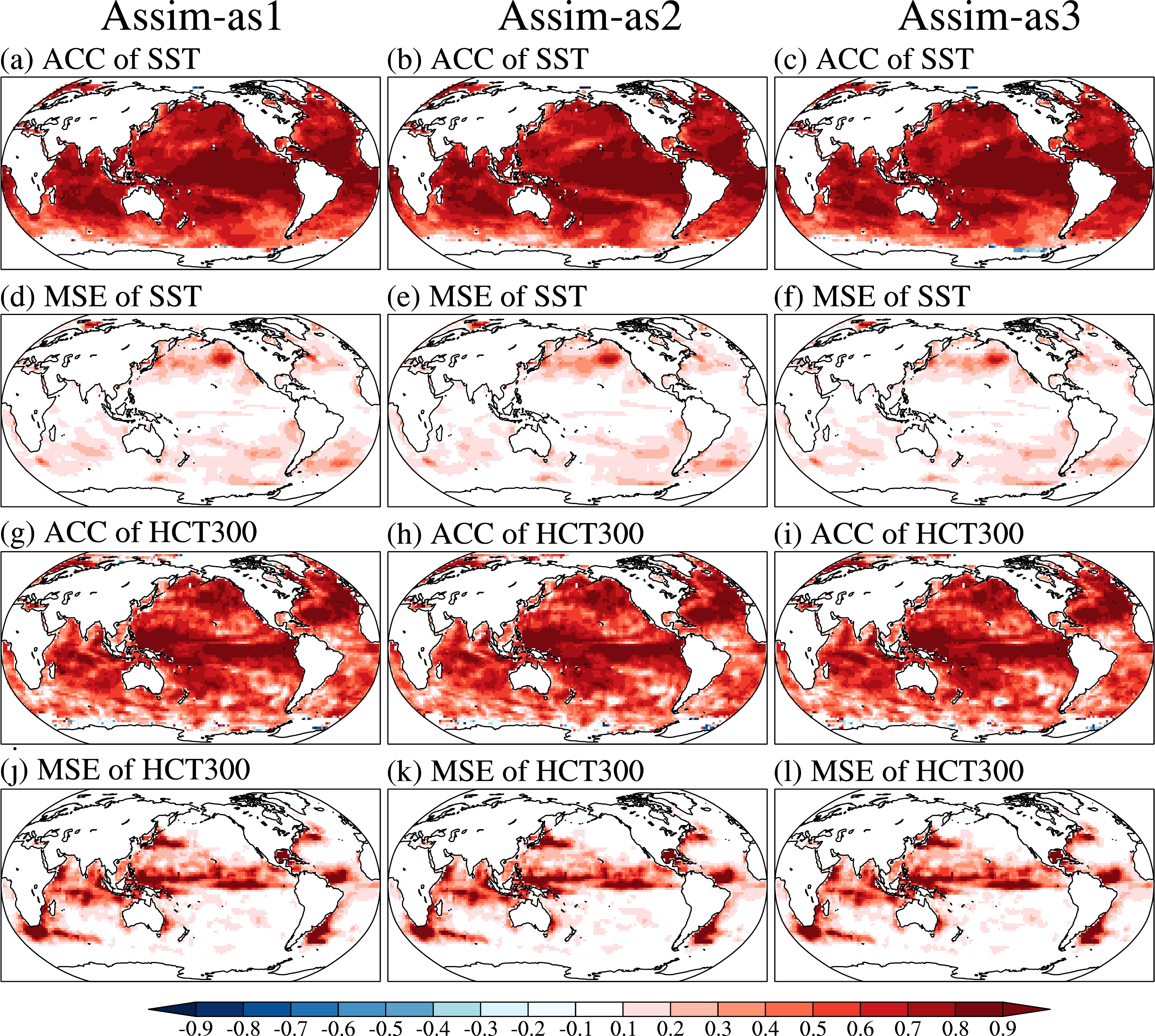
We first evaluate the accuracy of the initial conditions derived from the assimilation experiments. The ACC and MSE of the November SST anomaly (SSTA) and the total ocean heat content in the upper 300 m (HCT300) are shown in Fig. 1. The three assimilation experiments reproduce the observed variability of SSTA in the tropical central-eastern Pacific, the tropical Atlantic, and the tropical Indian Ocean well, with ACC greater than 0.8 and MSE less than 0.1°C. Compared with the tropics, there are larger biases for SSTA in the middle and high latitudes, especially in the northeastern Pacific (Figs. 1a–f). For the HCT300, the ACC in the tropical Pacific and the subtropical North Atlantic is higher than that in other sea areas (Figs. 1g–i), and large MSE is found mainly in the equator and coastal regions with the western boundary currents (Figs. 1j–l).

Figure 1. Accuracy of initial conditions provided by the assimilation runs. (a–c) ACC of November SSTA for three assimilation runs. (d–f) Mean squared error (MSE) of November SSTA for three assimilation runs (units: °C). (g–i) As in (a–c), but for ocean heat content from 0–300 m (HCT300). (j–l) As in (d–f), but for HCT300 (units: 1019 J).
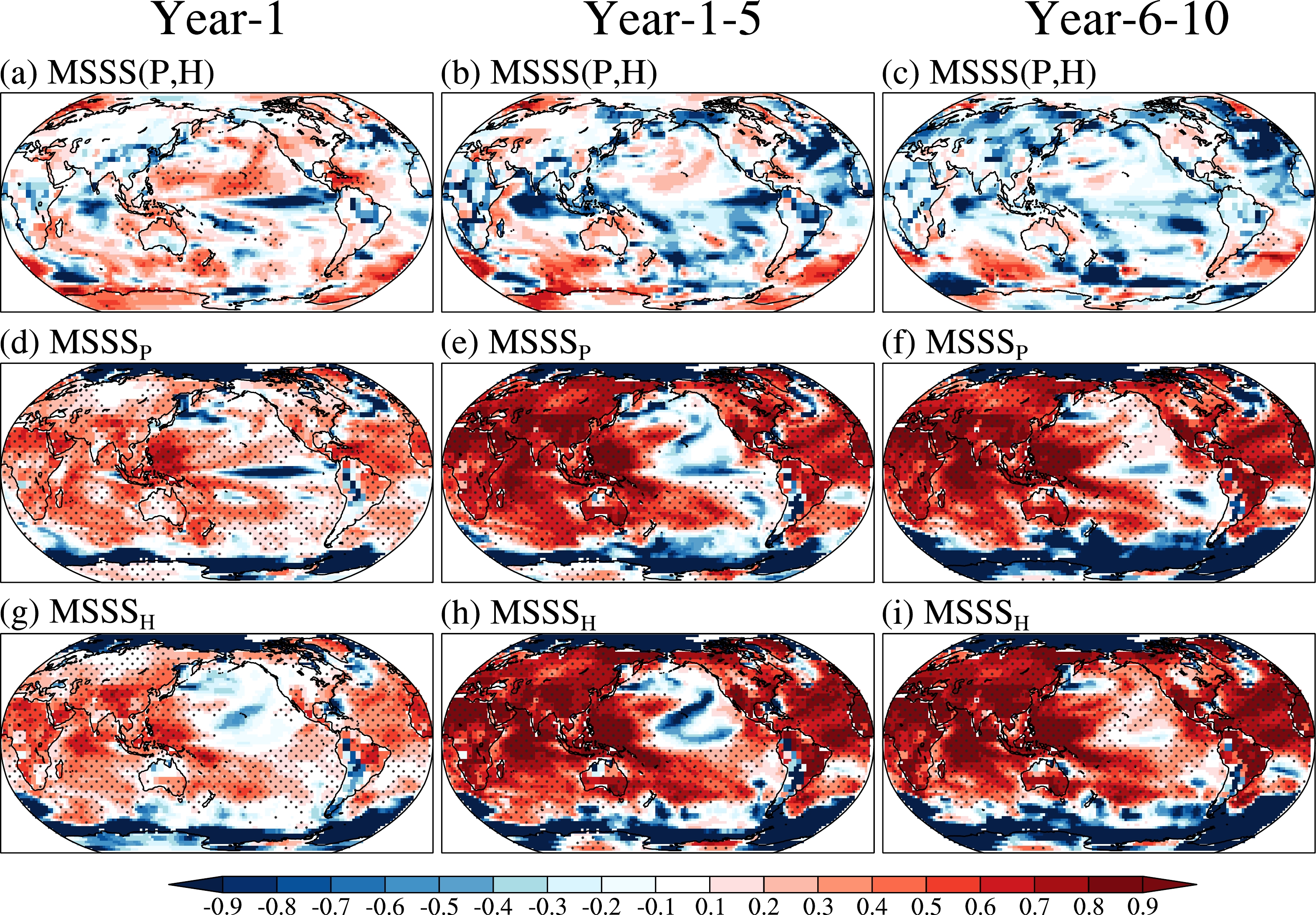
The MSSS of annual mean SST and land surface air temperature (SAT) anomalies is evaluated for forecast year 1, years 1–5, and years 6–10, respectively (Fig. 2). MSSS(P, H) indicates that the initialization significantly improves predictive skill of hindcast runs for year-1 SSTA in the north Pacific, the tropical Atlantic, the tropical southeastern Indian Ocean, and the Tasman sea relative to the uninitialized historical runs (Fig. 2a). For forecast years 1–5, the added value of initialization is mainly in the South Atlantic Ocean and the South Indian Ocean, while the improvement in the North Atlantic is limited (Fig. 2b). The spatial distribution of MSSS(P, H) for forecast years 6–10 is similar to that for forecast years 1–5, except for the subpolar gyre of the North Atlantic (Fig. 2c). It is found that there is strong model drift in the subpolar gyre that causes a strong cold bias there (not shown). The predictive skill of the initialized predictions and the uninitialized simulations compared with the reference prediction of the climatological average measured by MSSS (
$ {\mathrm{M}\mathrm{S}\mathrm{S}\mathrm{S}}_{\mathrm{P}} $ and$ {\mathrm{M}\mathrm{S}\mathrm{S}\mathrm{S}}_{\mathrm{H}} $ ) is shown in Figs. 2d–i. Although there is no observational oceanic information coming into the uninitialized simulations, the specified historical external forcing generates long-term warming trends, which bring some predictive skill for the runs (Figs. 2g–i). Comparing$ {\mathrm{M}\mathrm{S}\mathrm{S}\mathrm{S}}_{\mathrm{P}} $ and$ {\mathrm{M}\mathrm{S}\mathrm{S}\mathrm{S}}_{\mathrm{H}} $ , we can find that the initializations have added value in some places, which are generally consistent with the areas with positive MSSS(P, H) (Figs. 2d–f).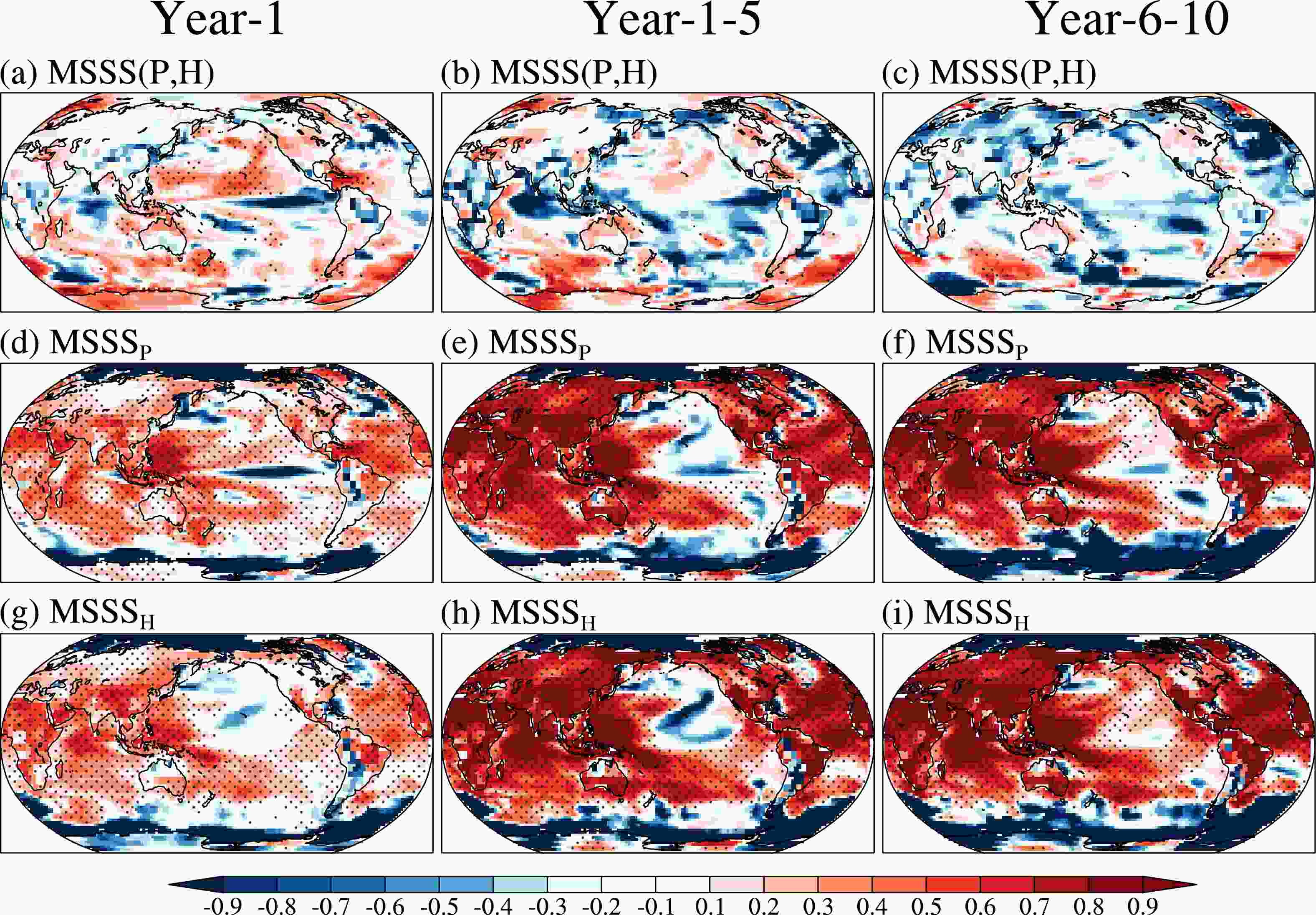
Figure 2. Predictive skill for annual mean sea surface temperature (SST) and land surface air temperature measured by mean squared skill score (MSSS). (a–c)
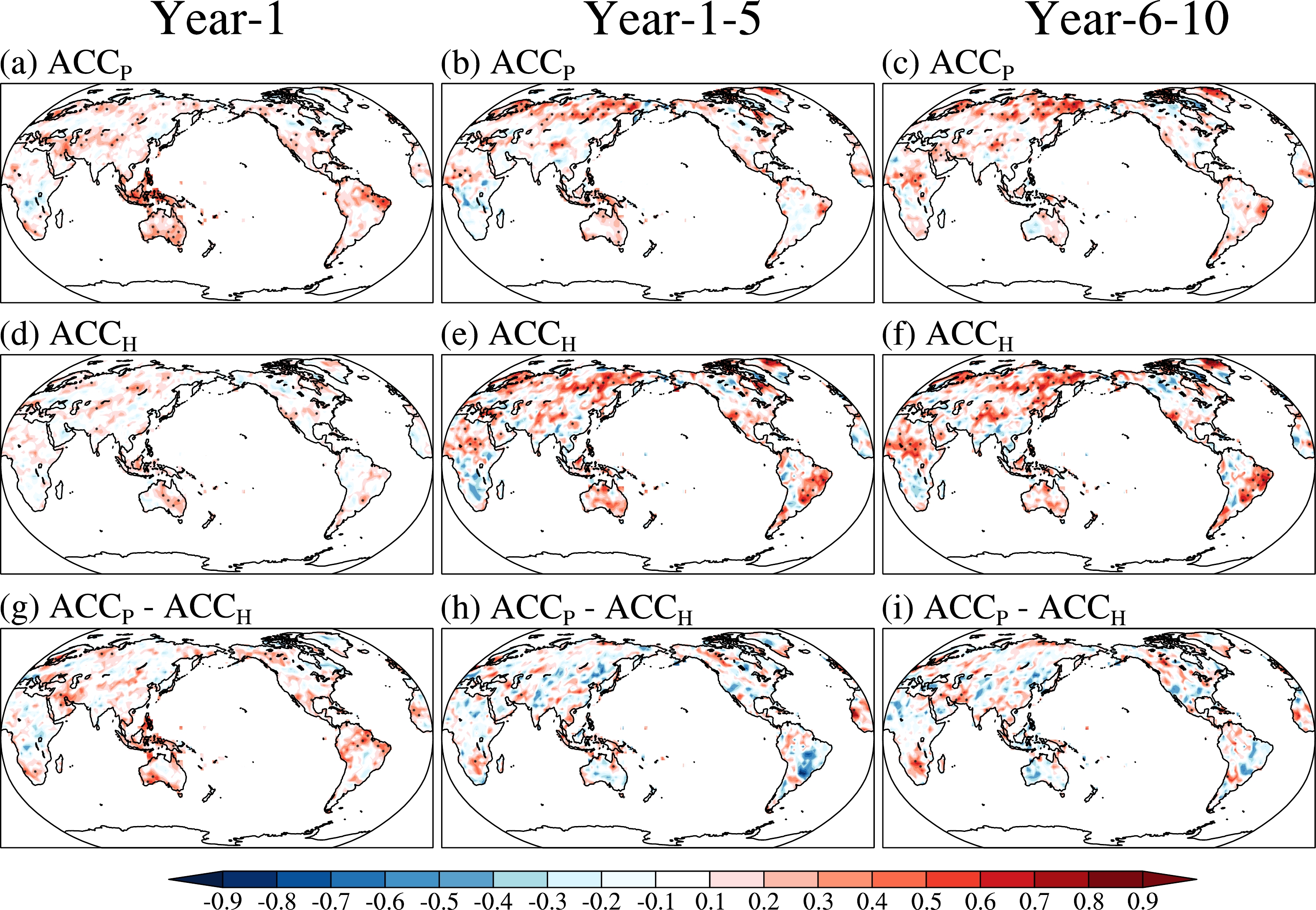
$ \mathrm{M}\mathrm{S}\mathrm{S}\mathrm{S}\left(\mathrm{P},\mathrm{H}\right) $ for forecast (a) year 1, (c) years 1–5, and (e) years 6–10. (d–f) As in (a–c), but for$ {\mathrm{M}\mathrm{S}\mathrm{S}\mathrm{S}}_{\mathrm{P}} $ . (g–i) As in (a–c), but for$ {\mathrm{M}\mathrm{S}\mathrm{S}\mathrm{S}}_{\mathrm{H}} $ . P (H) represents the initialized predictions (the uninitialized simulations).$ \mathrm{M}\mathrm{S}\mathrm{S}\mathrm{S}\left(\mathrm{P},\mathrm{H}\right) $ measures the improvement in accuracy of the initialized predictions over the reference prediction of the uninitialized simulations.$ {\mathrm{M}\mathrm{S}\mathrm{S}\mathrm{S}}_{\mathrm{P}} $ ($ {\mathrm{M}\mathrm{S}\mathrm{S}\mathrm{S}}_{\mathrm{H}} $ ) measures the improvement in accuracy of the initialized predictions (uninitialized simulations) over the reference prediction of the climatological average. Stippling shows where skill is statistically significant with 95% confidence.The ACC skill for annual mean SST and SAT is further evaluated (Fig. 3). For forecast year 1, significant positive ACCs of the initialized predictions are seen globally, with the highest skill located at the Indo–Pacific warm pool and tropical Atlantic (Fig. 3a). The added value of initialization on prediction skill is investigated using the difference in the ACC between the initialized prediction (
$ {\mathrm{A}\mathrm{C}\mathrm{C}}_{\mathrm{P}} $ ) and uninitialized simulations ($ {\mathrm{A}\mathrm{C}\mathrm{C}}_{\mathrm{H}} $ ) (Fig. 3d).$ {\mathrm{A}\mathrm{C}\mathrm{C}}_{\mathrm{P}} $ is significantly improved in the North Pacific, the Tasman sea, the Scotia sea, and the subpolar gyre of the North Atlantic relative to$ {\mathrm{A}\mathrm{C}\mathrm{C}}_{\mathrm{H}} $ (Fig. 3g). For the multi-year predictions, both ACCP and$ {\mathrm{A}\mathrm{C}\mathrm{C}}_{\mathrm{H}} $ are driven by the long-term trend of surface temperature, and their difference shows that the improvements resulting from the initialization are very limited (Figs. 3b, e, h, and c, f, i).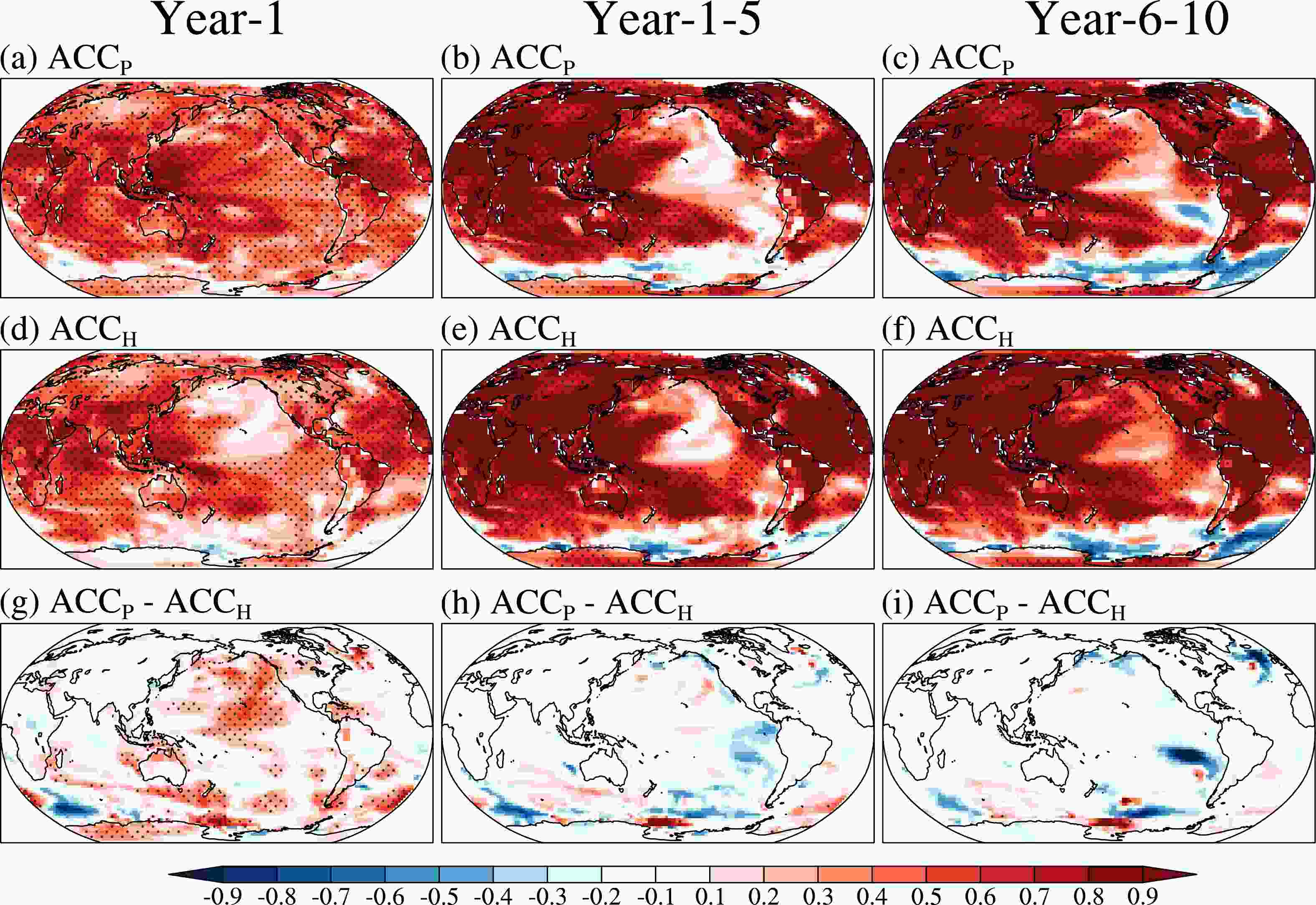
Figure 3. Predictive skill for SST and land SAT measured by ACC. (a–c)
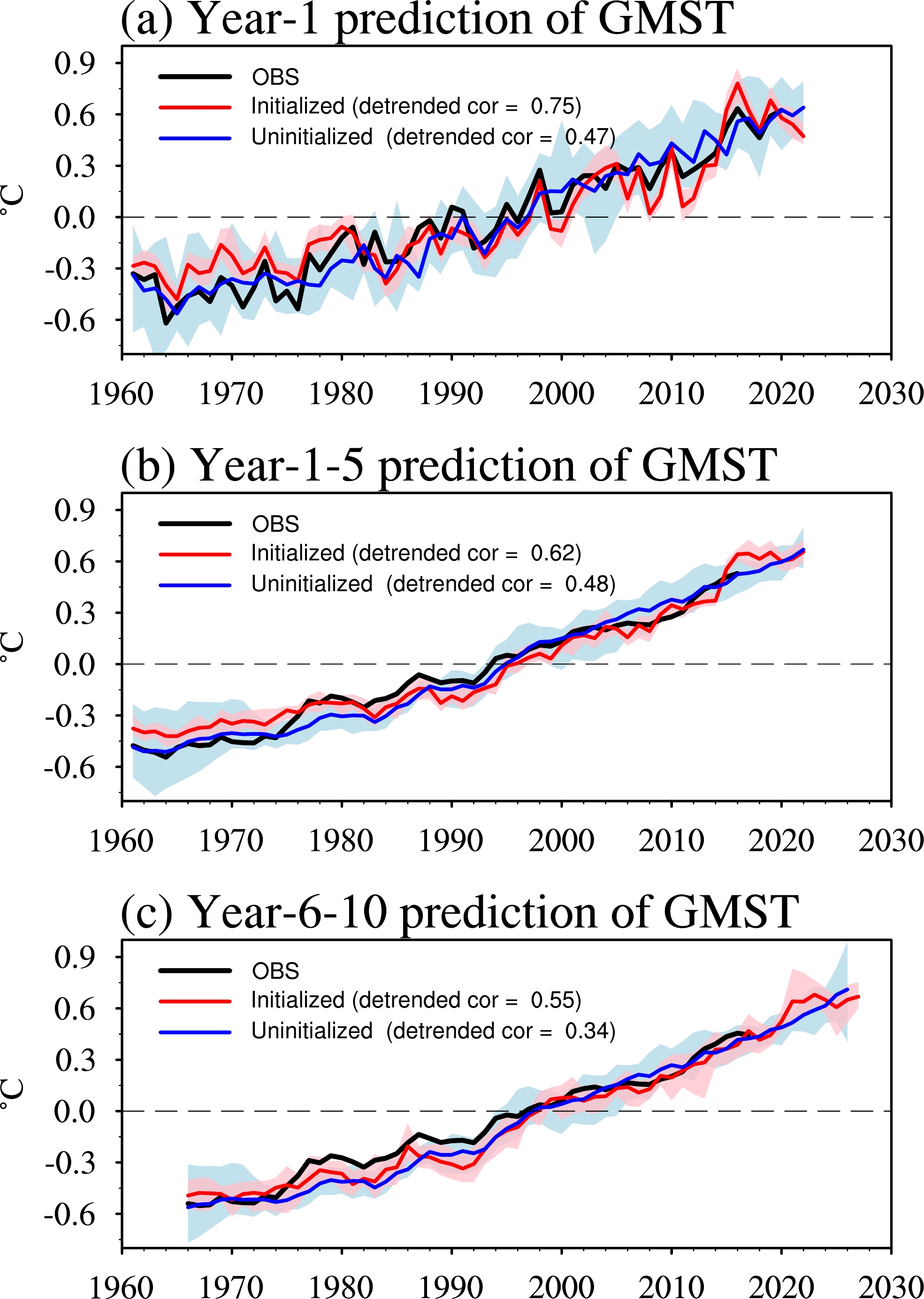
$ {\mathrm{A}\mathrm{C}\mathrm{C}}_{\mathrm{P}} $ for forecast (a) year 1, (c) years 1–5, and (e) years 6–10. (d–f) As in (a–c), but for$ {\mathrm{A}\mathrm{C}\mathrm{C}}_{\mathrm{H}} $ . (g–i) As in (a–c), but for the difference of$ {\mathrm{A}\mathrm{C}\mathrm{C}}_{\mathrm{P}} $ and$ {\mathrm{A}\mathrm{C}\mathrm{C}}_{\mathrm{H}} $ .$ {{\mathrm{A}\mathrm{C}\mathrm{C}}_{\mathrm{P}}}_{} $ ($ {\mathrm{A}\mathrm{C}\mathrm{C}}_{\mathrm{H}} $ ) is the correlation coefficient between the observed and initialized predicted (uninitialized simulated) anomalies. Stippling shows where skill is statistically significant with 95% confidence.The global mean surface temperature (GMST) is a frequently used metric to measure global climate change, and thus we further show the prediction of the annual mean GMST averaged over forecast year 1, years 1–5, and years 6–10 (Fig. 4). For forecast year 1, the initialized prediction shows much higher skill in reproducing the interannual variability of GMST than the uninitialized simulations, with their correlation coefficients of the detrended GMST with the observation being 0.75 and 0.47, respectively (Fig, 4a). Here, linear detrending is directly applied to GMST indices for the entire period. For forecast years 1–5 and years 6–10, the initialized predictions are more skillful than the uninitialized simulations, with the former detrended correlation with the observation being much higher than the latter (Figs. 4b, c). It is also noted that the ensemble spreads (defined as the range between the minimum and maximum values across the ensemble) of the initialized predictions are much smaller than those of the uninitialized simulations, especially for forecast year 1 and years 1–5.
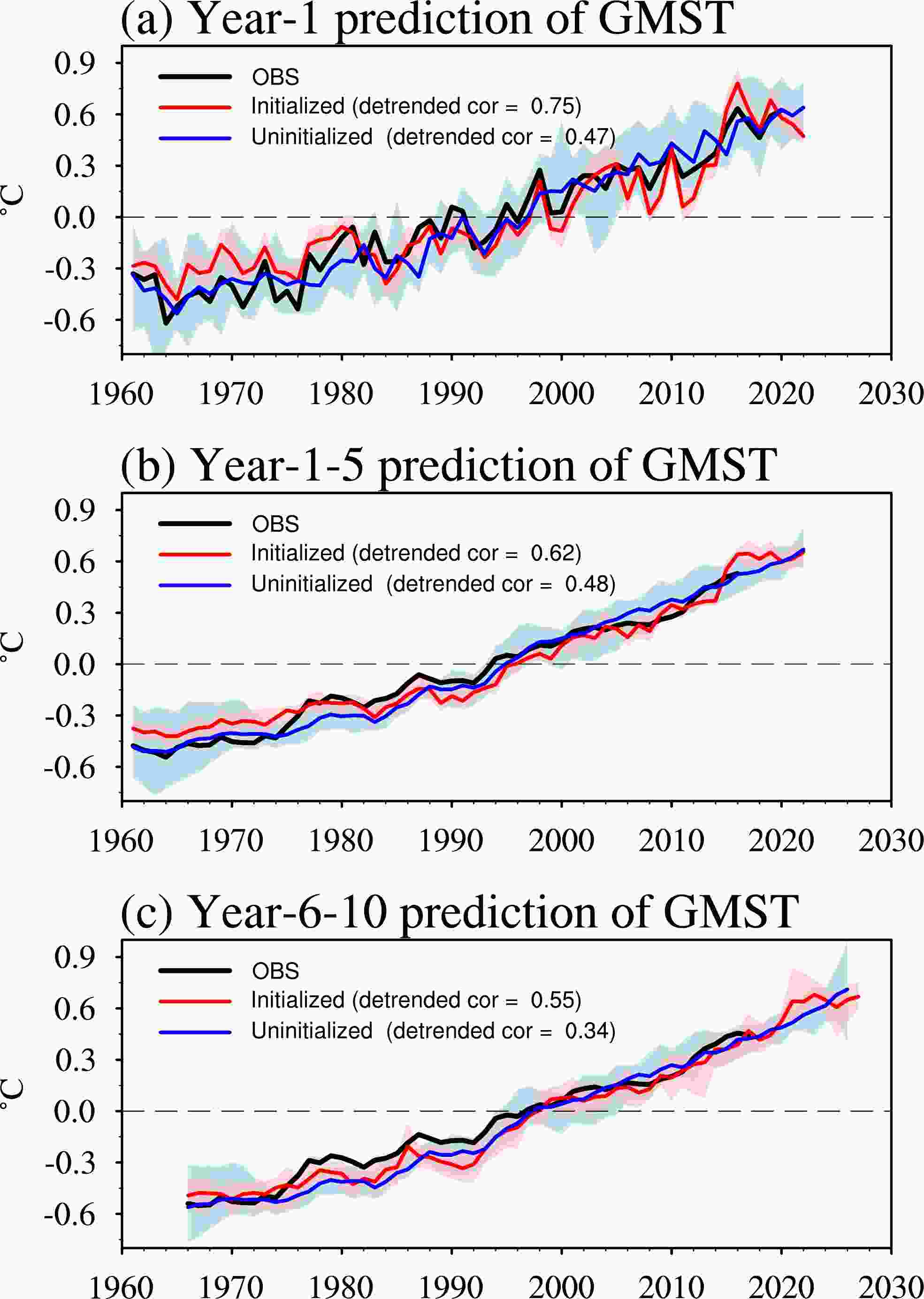
Figure 4. Predictions of global mean surface air temperature (GMST) for forecast year 1 (a), years 1–5 (c), and years 6–10 (e). The black line represents the observation. The red (blue) line represents the ensemble mean of the initialized predictions (the uninitialized historical runs). The red and blue shadings are the ensemble spreads, which are defined as the range between the minimum and maximum values across the ensemble.
Finally, we assess ACC skill for annual mean land precipitation and sea level pressure (SLP) anomalies. Compared with that for surface temperature, the predictive skill for land precipitation is much lower. And the improvements of the initialized predictions relative to the uninitiated simulations are very scattered (Fig. 5), which is consistent with previous studies (Doblas-Reyes et al., 2013). The predictive skill for SLP is relatively high for forecast year 1 (Fig. 6a). The ACC skill of the initialized runs is significantly higher than that of the uninitialized simulations over the tropics and extratropical Northern Hemisphere, which suggests that the initialization remarkably improves predictive skill associated with ENSO variability (Figs. 6d, g). For forecast years 1–5 and 6–10, the initialized predictions show higher ACC over the extratropical North Pacific. But in other ocean areas, the improvement for SLP decadal predictive skill due to initialization is not significant (Figs. 6h, i).
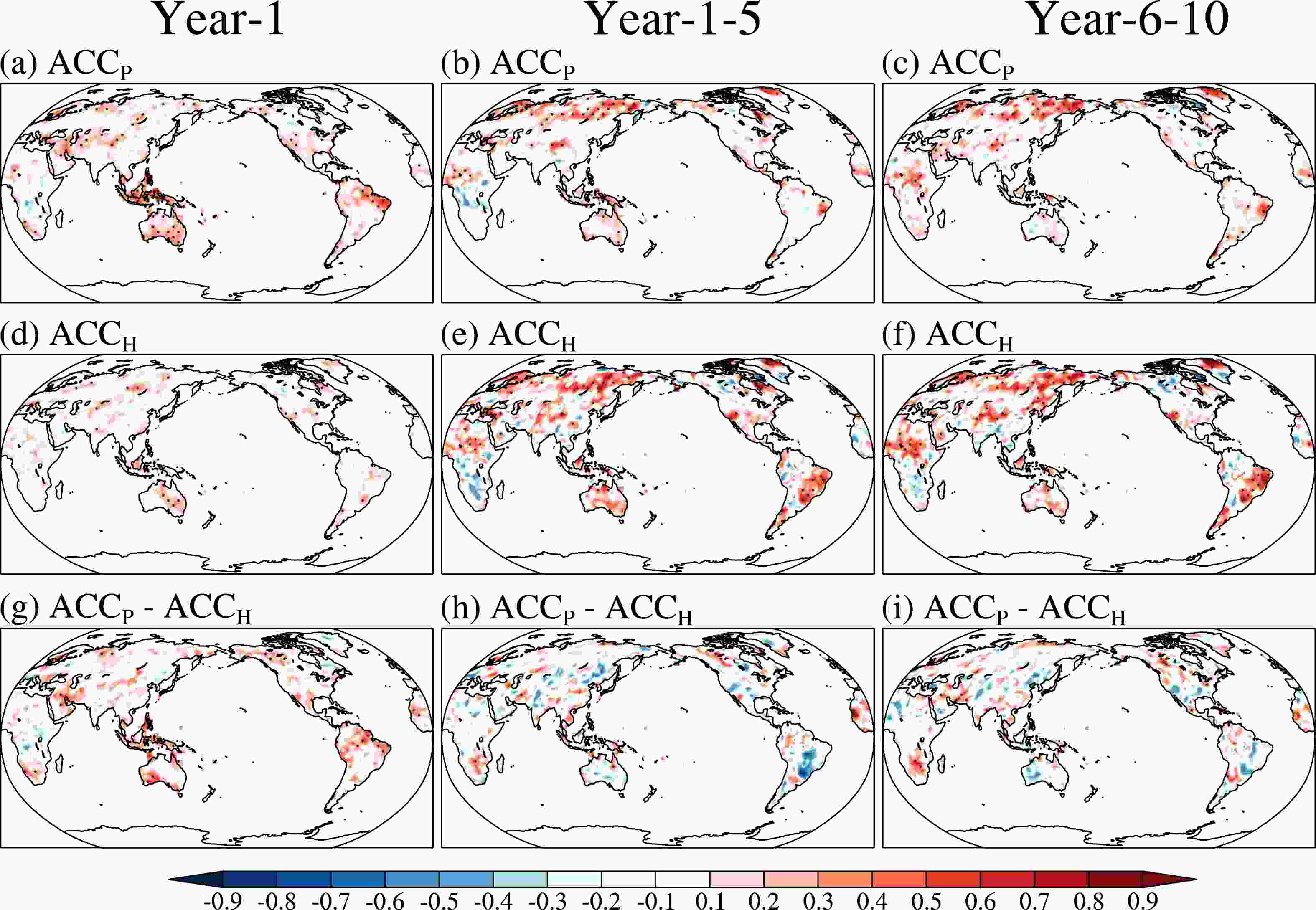
Figure 5. Predictive skill for annual mean land precipitation measured by ACC. (a–c) ACC of the nine-member ensemble mean of the initialized prediction runs for forecast year 1 (a), years 1–5 (c), and years 6–10. (d–f) As in (a–c), but for the historical runs. (g–i) The differences of ACC between the initialized runs and the historical runs. Stippling represents that skill is significant at the 5% level.
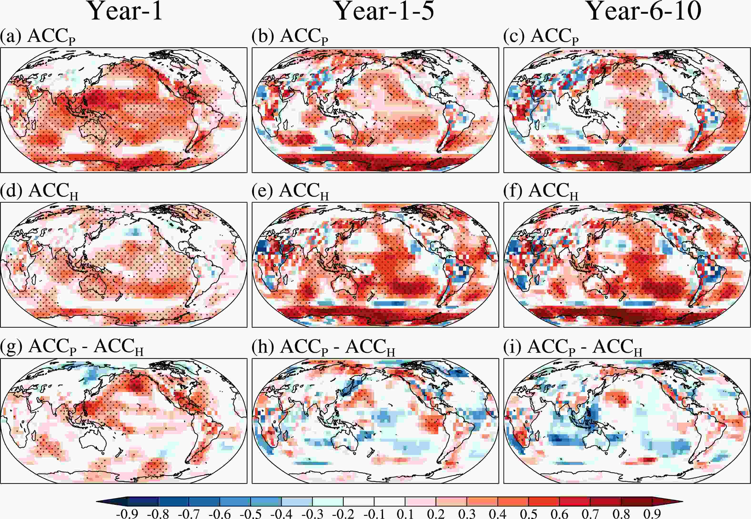
Figure 6. As in Fig. 5, but for annual mean sea level pressure.
In addition to the assessments shown above, there are some other assessment approaches for decadal predictions, such as partial ACC proposed by Smith et al. (2019), with a focus on the added value of decadal prediction on internal variability. This approach relies on large-ensemble simulations to separate internal variability and externally forced variability, which could not be achieved here because of the small ensemble size. In the future, we would further improve the initialization scheme and increase ensemble size to offer decadal prediction results with more robust and reliable predictive skill.
-
A full list of CAS FGOALS-f3-L output variables for CMIP6 DCPP component-A and component-B experiments is given in Table 2. All the variables are archived at a monthly time scale. The original atmospheric model grid is in the cube-sphere grid system with a resolution of C96, which has six tiles and is irregular in the horizontal direction. We merged and interpolated the six tiles to a global latitude–longitude grid with a nominal resolution of 1° using one-order conservation interpolation as required by CMIP6, and transformed the atmospheric three-dimension variables from the model layers to pressure levels, following He et al. (2019).
Output name Description Units hfls Surface Upward Latent Heat Flux W m−2 hfss Surface upward sensible heat flux W m−2 hur Relative Humidity % hus Specific Humidity kg kg−1 pr Precipitation kg m−2 s−1 ps Surface air pressure Pa psl Sea level pressure Pa ta Air temperature K tas Near-surface air temperature K ts Surface temperature K ua Eastward wind m s−1 va Northward wind m s−1 zg Geopotential height m tos Sea Surface Temperature °C tob Sea Water Potential Temperature at Sea Floor °C uo Sea Water X Velocity m s−1 vo Sea Water Y Velocity m s−1 wo Sea Water Vertical Velocity m s−1 so Sea Water Salinity psu thetao Sea Water Potential Temperature °C sos Sea Surface Salinity psu zos Sea Surface Height Above Geoid m sossq Square of Sea Surface Salinity 10-6 friver Water Flux into Sea Water from Rivers kg m−2 s−1 hfbasinpmdiff Northward Ocean Heat Transport Due to Parameterized Mesoscale Diffusion W hfsso Surface Downward Sensible Heat Flux W m−2 msftbarot Ocean Barotropic Mass Streamfunction kg s−1 rlntds Surface Net Downward Longwave Radiation W m−2 sob Sea Water Salinity at Sea Floor psu tauuo Surface Downward X Stress N m−2 wfo Water Flux into Sea Water kg m−2 s−1 zossq Square of Sea Surface Height Above Geoid m2 hfbasin Northward Ocean Heat Transport W hfds Downward Heat Flux at Sea Water Surface W m−2 msftmz Ocean Meridional Overturning Mass Streamfunction kg s−1 rsntds Net Downward Shortwave Radiation at Sea Water Surface W m−2 tauvo Surface Downward Y Stress N m−2 hfbasinpmadv Northward Ocean Heat Transport Due to Parameterized Mesoscale Advection W hflso Surface Downward Latent Heat Flux W m−2 mlotstsq Square of Ocean Mixed Layer Thickness Defined by Sigma T m2 msftmzmpa Ocean Meridional Overturning Mass Streamfunction Due to Parameterized Mesoscale Advection kg s−1 tossq Square of Sea Surface Temperature °C2 vsf Virtual Salt Flux into Sea Water kg m−2 s−1 mlotst Ocean Mixed Layer Thickness Defined by Sigma T m Table 2. CAS FGOALS-f3-L output variables prepared for CMIP6 DCPP component-A and component-B experiments.
The orthogonal curvilinear coordinate is introduced into LICOM3, and thus the oceanic variables are on the original tripolar grid, with the North Pole split into two poles on two continents at (35°N, 114°E) and (35°N, 66°W), respectively. The oceanic variables have 360 grid cells in the zonal direction and 218 grid cells in the meridional direction (approximately equal to 1° at a globally horizontal resolution), with uneven enhanced meridional resolution from 0.5° to 1° near the equator. For the oceanic vector variables, the resolution is 30 layers, which are 10 m per layer in the upper 150 m and divided into uneven vertical layers below 150 m. In addition, since the horizontal oceanic vector is on the orthogonal curvilinear coordinate, it needs to be rotated according to the angles between the original grid and the latitude–longitude grid before interpolation.
The format of datasets is the version 4 of Network Common Data Form (NetCDF), which can be easily read and written by professional common software such as NetCDF Operator (
http://nco.sourceforge.net ), NCAR Command Language (http://www.ncl.ucar.edu ), Python (https://www.python.org ), and Climate Data Operators (https://www.unidata.ucar.edu/software/netcdf/workshops/most-recent/third_party/CDO.html ). According to regulations of CMIP6, the data collection should follow the Data Citation Guidelines (http://bit.ly/2gBCuqM ) and be sure to include the version number. Individuals using the data must abide by terms of use for CMIP6 data (https://pcmdi.llnl.gov/CMIP6/TermsOfUse ).Acknowledgements. This work is jointly supported by National Key Research and Development Program of China (Grant No. 2018YFA0606300), the NSFC (Grant No. 42075163), the NSFC BSCTPES project (Grant No. 41988101), and the NSFC (Grant No. 42205039). This work is also supported by the Jiangsu Collaborative Innovation Center for Climate Change and the National Key Scientific and Technological Infrastructure project “Earth System Science Numerical Simulator Facility” (EarthLab).
Data availability statement. The data that support the findings of this study are available from
https://esgf-node.llnl.gov/projects/cmip6/ . The HadCRUT.5.0.1.0 dataset can be downloaded fromhttps://www.metoffice.gov.uk/hadobs/hadcrut5/data/current/download.html . The GPCC dataset can be downloaded fromhttps://psl.noaa.gov/data/gridded/data.gpcc.html . The ERSST dataset can be downloaded fromhttps://www.ncei.noaa.gov/pub/data/cmb/ersst/v5/netcdf/ . The HadSLP2 dataset can be downloaded fromhttps://www.metoffice.gov.uk/hadobs/hadslp2/ .Disclosure statement.
No potential conflict of interest was reported by the authors. Open Access This article is licensed under a Creative Commons Attribution 4.0 International License, which permits use, sharing, adaptation, distribution and reproduction in any medium or format, as long as you give appropriate credit to the original author(s) and the source, provide a link to the Creative Commons licence, and indicate if changes were made. The images or other third party material in this article are included in the article’s Creative Commons licence, unless indicated otherwise in a credit line to the material. If material is not included in the article’s Creative Commons licence and your intended use is not permitted by statutory regulation or exceeds the permitted use, you will need to obtain permission directly from the copyright holder. To view a copy of this licence, visit
http://creativecommons.org/licenses/by/4.0/ .
| Database profile | |
| Database title | CAS FGOALS-f3-L Model Datasets for CMIP6 DCPP Experiment |
| Time range | dcppA-hindcast: 1960–2016 dcppB-forecast: 2017–21 |
| Geographical scope | dcppA-hindcast: global dcppB-forecast: global |
| Data format | version 4 of Network Common Data Form (NetCDF) |
| Data volume | 4.07 TB for dcppA-hindcast 351GB for dcppB-forecast |
| Data service system | |
| Sources of funding | The National Key Research and Development Program of China (Grant No. 2018YFA0606300), the NSFC (Grant No. 42075163), the NSFC BSCTPES project (Grant No. 41988101), and the NSFC (Grant No. 42205039) |
| Database composition | 1. The dcppA-hindcast comprises nine-member hindcasts initialized on 25, 28, and 30 November for each year during 1960–2016, containing 44 monthly mean atmospheric and oceanic variables.2. The dcppB-hindcast comprises nine-member hindcasts initialized on 25, 28, and 30 November for each year during 2017–21, containing 44 monthly mean atmospheric and oceanic variables. |


 AAS Website
 AAS WeChat