


 DownLoad:


-
Extreme cold events over East Asia are some of the most frequent climate disasters in winter. Accumulated evidence implies that extreme cold waves have become more severe and frequent over the midlatitudes in recent years. For example, record-breaking low temperatures and strong blizzards affected many regions in East Asia during the 2010/11 winter (Gong et al., 2014). A strong cold event, commonly known as a “boss level” cold wave, affected East Asia in January 2016, with many observation stations setting their lowest daily temperature records (Cheung et al., 2016; Song and Wu, 2017; Qian et al., 2018; Ma and Zhu, 2019; Yamaguchi et al., 2019). Moreover, three extreme cold air invasion events from December 2020 to mid-January 2021 resulted in drastic temperature drops in China (Dai et al., 2022; Zheng et al., 2022).
Some studies have suggested that the frequent cold extremes occurring in Eurasia, North America, and East Asia (Francis and Vavrus, 2012; Liu et al., 2012; Tang et al., 2013; Cohen et al., 2014; Mori et al., 2014; Kug et al., 2015; Overland et al., 2015; Cheung et al., 2018; Zhang et al., 2020) are associated with the loss of Arctic sea ice through the promotion of more blocking events and the subsequent intrusions of Arctic air into the midlatitudes. The frequent outbreaks of cold extremes in recent years are related to the rapid ice retreat in the Barents–Kara (B–K) Seas, which triggers adjustments in the atmospheric circulation that affect regions at midlatitudes through the Arctic Oscillation (AO)/North Atlantic Oscillation (NAO) and/or Siberian High (SH) (e.g., Honda, et al., 2009; Wu et al., 2011; Inoue et al., 2012; Tang et al., 2013; Cheung et al., 2018). However, some studies have argued that the frequent occurrence of the midlatitude cold extremes is due to internal variability and has no causal relationship with the Arctic sea ice retreat (Barnes, 2013; Barnes and Screen, 2015; McCusker et al., 2016; Sun et al., 2016). Scientists have noticed that the determination of whether a decline of Arctic sea ice significantly influences midlatitude weather may depend on the time scale (Mu et al., 2022). Previous studies have pointed out that the impact of Arctic sea ice decline on the midlatitude atmospheric circulation and associated cold extremes is less important to the long-term trend or on interdecadal time scales, while it is evident on the interannual and seasonal time scales (Luo et al., 2016; Dai and Song, 2020). However, due to the short record of observed data, large uncertainty still exists about whether Arctic sea ice influences midlatitude cold extremes.
There are abundant historical documents and paleoclimatic data that can provide a rich base of data for the study of extreme winter cold waves in China. Most of the proxies have high spatial and temporal resolutions and clear climatic indications. Ge et al. (2003) quantitatively reconstructed the winter temperature time series in eastern China during the last 2000 years using cold and warm records from historical documents. By examining the characteristics of cold winters in eastern China during the historical period, Wang (2008) found that the winter of 2008 was the coldest one since 1977, and 7% of the winters met the threshold of severe (winter temperature anomaly reaches –2.5°C) winters during the period 1880–2007. Hao et al. (2012) and Ding et al. (2016) reconstructed the temperature time series since 1736 of the area downstream of the Yangtze River and southern China by using the record of “Rain and Snow Scale” and other ancient literature records from the Qing Dynasty. Based on historical records of the southern extents of frost events, freezing events, snow, snowfall days, and first/late frost dates, Zheng et al. (2018) reconstructed the winter temperature time series for southern China over the past 500 years. Yan et al. (2014) reconstructed the winter temperature time series since 1645 with 5-year resolution for northern China based on records of abnormal frost and snow disasters in the local Chronicles of the Qing Dynasty.
Most previous studies were focused on the average temperature in winter; few of them referred to winter extreme cold events. Zheng et al. (2014) investigated 76 extreme cold events that occurred from 1500 to 1950, most of which were more significant than those occurring after 1950. However, extreme cold event reconstructions still have large uncertainties about them because of different proxies and reconstruction criterion and inconsistent time periods. In this study we investigate the influence of Arctic sea ice on midlatitude extreme cold events from a historical perspective. Based on historical documents, we reconstruct the time series of the winter extreme cold index of southern China to examine its relationship with Arctic sea ice under different climatic backgrounds during the past ~700 years. We further discuss the possible mechanisms associated with atmospheric circulation. This study helps advance our understanding of how Arctic sea ice change contributes to the occurrence of extreme cold events in China.
-
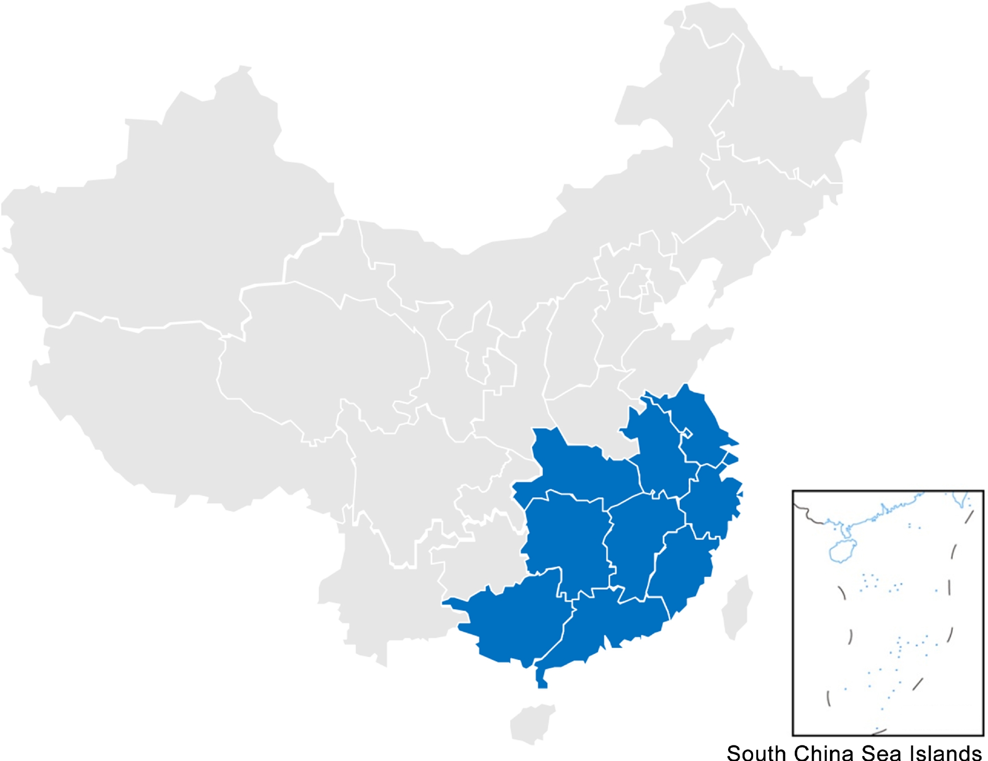
Extreme cold events in China were extracted from “A Compendium of Chinese Meteorological Records of the Last 3000 years” (Zhang, 2013), which was quoted from 48 ancient Chinese books subjected to systematic collection and rectification. More than 8000 historical documents were studied, and over 200 000 weather-related records were evaluated. All the records in the compendium have been geographically verified to ensure that the documented locations are generally consistent with the current administrative provinces (Zhang et al., 2003; Zhang, 2005). The ancient site names have been translated to their present-day names based on “The Historical Atlas of China” (Tan, 1987). In this study, the historical period is selected from 1289 to 1911, covering the dynasties of Yuan, Ming, and Qing. We focus on extreme cold wave events (ECWEs) by referring to the “boss level” cold wave in 2016; ECWEs are characterized by extreme intensity, wide influential range, long duration, and often a tendency to move south of the “Qinling-Huaihe Line” to affect southern China. Therefore, we collected the historical records of 10 provinces/province-level municipalities including Anhui, Zhejiang, Jiangxi, Hunan, Shanghai, Jiangsu, Fujian, Hubei, Guangdong, and Guangxi (Fig. 1). The records selected for this study were also compared with the climate records of the historical Chinese dynasties and other related references (e.g., Gong and Wang 1999; Wang et al., 1999; Wang, 2008; Hao et al., 2012; Yan et al., 2014; Zheng et al., 2014; Ding et al., 2016).
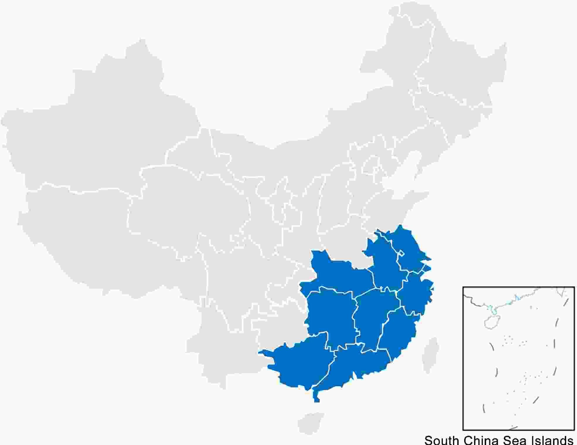
Figure 1. The geographical range of provinces/province-level municipalities included in the strong cold wave records used for this study (blue filled area).
-
ECWEs during the instrumental period (1872–2017) were estimated from reanalysis data. Daily average 2-m temperatures were extracted from the NCEP-DOE reanalysis 2 (1979 to present,
https://www.esrl.noaa.gov/psd/data/gridded/data.ncep.reanalysis2.html ) and NOAA-CIRES-DOE Twentieth Century Reanalysis (20CR) Version 2 (1871–2012,https://www.esrl.noaa.gov/psd/data/gridded/data.20thC_ReanV2.html ). The NOAA-CIRES-DOE data was used to estimate the ECWEs from 1872 to 1979, and NCEP-DOE data was used to estimate the ECWEs from 1980 to 2017. In this study, the domain of 22°–35°N, 107°–124°E was selected to represent southern China and to coincide with the area covered by the historical records. Winter season refers to the period from December to February of the following year. -
The B–K Seas are considered to be a key area affecting cold winter extremes over Eurasia and east Asia because the sea ice decline in this region can increase the quasi-stationarity and persistence of Ural blocking (Yao et al., 2017), which favors Eurasian cold extremes by reducing the meridional background potential vorticity gradient (Luo et al., 2019). The autumn sea ice extent (SIE) over the B–K Seas from 1289 to 1993 reconstructed by Zhang et al. (2018b) was used here to investigate correlations with the occurrence of extreme cold events in southern China. The observed SIE data from 1981 to 2017 was obtained from the National Snow & Ice Data Center (
http://nsidc.org/data/masie ).The SH index (SHI) and NAO index (NAOI) were used to understand the potential connection between sea ice and cold events. Both the observed and reconstructed data were applied. The observed winter SHI was calculated by the averaged sea level pressure in the domain 40°–60°N, 80°–120°E, and the long-term time series from 1599–1980 was obtained from the reconstruction by D'Arrigo et al. (2005). The observed NAOI was obtained from HURRELL (
https://climatedataguide.ucar.edu/climate-data/hurrell-north-atlantic-oscillation-nao-index-station-based ). The reconstructed NAOI came from Trouet et al. (2009), which cover the period 1049–1995. -
In order to quantify cold event records contained in literature into intensity levels of ECWEs, we marked the contents in the historical documents according to the following five criteria: “snow and snow freeze for more than 10 days”, “snow depth description”, “river and lake freeze”, “livestock/crop freeze to death”, and “human freeze to death”. By referring to the method of quantifying events in the historical record into cold degrees by Wang and Wang (1990), we recorded the cold event intensity of each year. Level 0 denotes normal winter descriptions, such as “heavy snow in January”, “heavy snow”, etc; Level 1 represents general abnormal cold, which meets about two of the above five criteria; Level 2 refers to extreme cold of a heavier degree, which generally satisfies more than two of the above criteria.
Although using the five criteria allowed us to classify the ECWEs, their cold wave intensity still could not be defined due to the incompleteness, inhomogeneity, and irregularity of ancient literature. Some weather condition descriptions were too brief to evaluate the actual ECWE intensity in the given year. For the sake of uniformity, some simple records were classified as Level 0. Finally, the chronology of the occurrence year and corresponding intensity of the ECWEs in the history of 10 provinces/province-level municipalities in southern China was built.
In order to ensure uniformity of results, the same statistical standard was adopted for all regions. However, for similar cold wave events, their intensities were usually recorded using different descriptions depending on the region. For example, descriptions of river or lake freezes usually corresponded to different cold degrees between Guangdong and Anhui provinces. In general, cold waves arriving to Guangdong, Guangxi, and Fujian provinces were more severe. Therefore, we increased the weight of cold wave records from Guangdong, Guangxi, and Fujian by a factor of 0.5. The intensity of an ECWE was usually defined as the average between all the areas where it was recorded. But this ignored the important fact that more places with ECWE records also means a higher probability of an ECWE occurring in a given year. Therefore, in order to characterize the intensity of ECWEs more realistically, we consider the number of areas with records as one of the impact factors and define the strong Cold Index as:
where
$ {X}_{i} $ represents the intensity of the ECWEs and n denotes the number of regions where ECWEs were recorded. Compared with the arithmetic average$ \left[\right(\sum _{i}{X}_{i})/n]\frac{}{} $ , the weight coefficient of$ [n/({\mathrm{log}}_{2}n+1\left)\right] $ can constrain the increase of n within a reasonable range. A higher n indicates a greater likelihood, intensity, and extent of an ECWE. -
Barnes (2013) reported that the correlation between Arctic sea ice and midlatitude cold winter events largely depends on the choice of analysis method and definition of extreme weather climate events. Ayarzagüena and Screen (2016) found that the frequency and duration of cold air outbreaks were not stable with Arctic sea ice, and their results were very sensitive to the definition standard of a cold air outbreak; the adoption of different definitions of ECWEs led to completely different conclusions. Therefore, it is necessary to discuss the definition of ECWEs in depth. Previous studies have defined strong cold events in terms of the temperature being less than 1.5 times the standard deviation with respect to the local climate state (Tang et al., 2013; Ou et al., 2015). Gong and Wang (1999) analyzed anomalously cold winters in China based on a threshold of 1.3 standard deviations (extreme cold events that occur one time every 10 years). Based on the criterion of temperature being lower than the climate state by 1.5 standard deviations, Song and Wu (2017) calculated 37 ECWEs during the winters of 1979–2016 in the south (20°–40°N, 100°–120°E) of China.
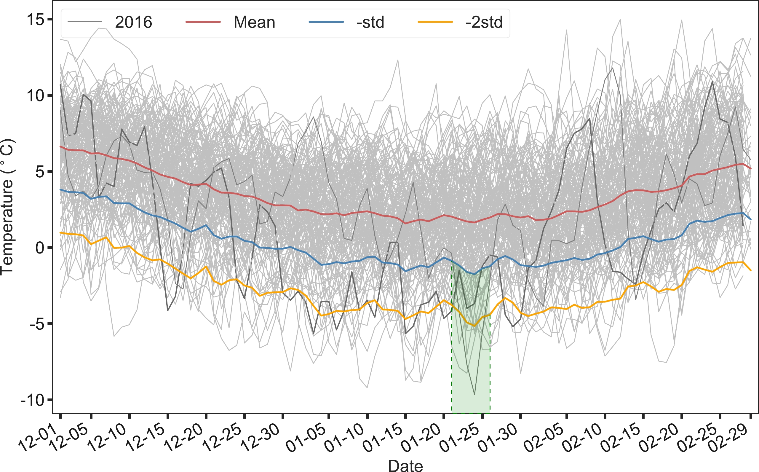
This study attempts to define a criterion for strong cold wave outbreaks that have occurred frequently in recent years by referring to the "boss level" cold wave which impacted East Asia in January 2016. As shown in Fig. 2, the "boss level" cold wave event in 2016 is an extremely rare event, which is characterized by being greater than two standard deviations below the climate state. With reference to the "boss level," we used three indicators to extract the ECWEs in the instrumental period, including the degree of temperature anomaly (less than two standard deviations), extreme low temperature (≤3°C), and cooling rate of daily temperature (≥3.5°C). Their time series were standardized and defined as: anomaly index, extremum index, and cooling index.
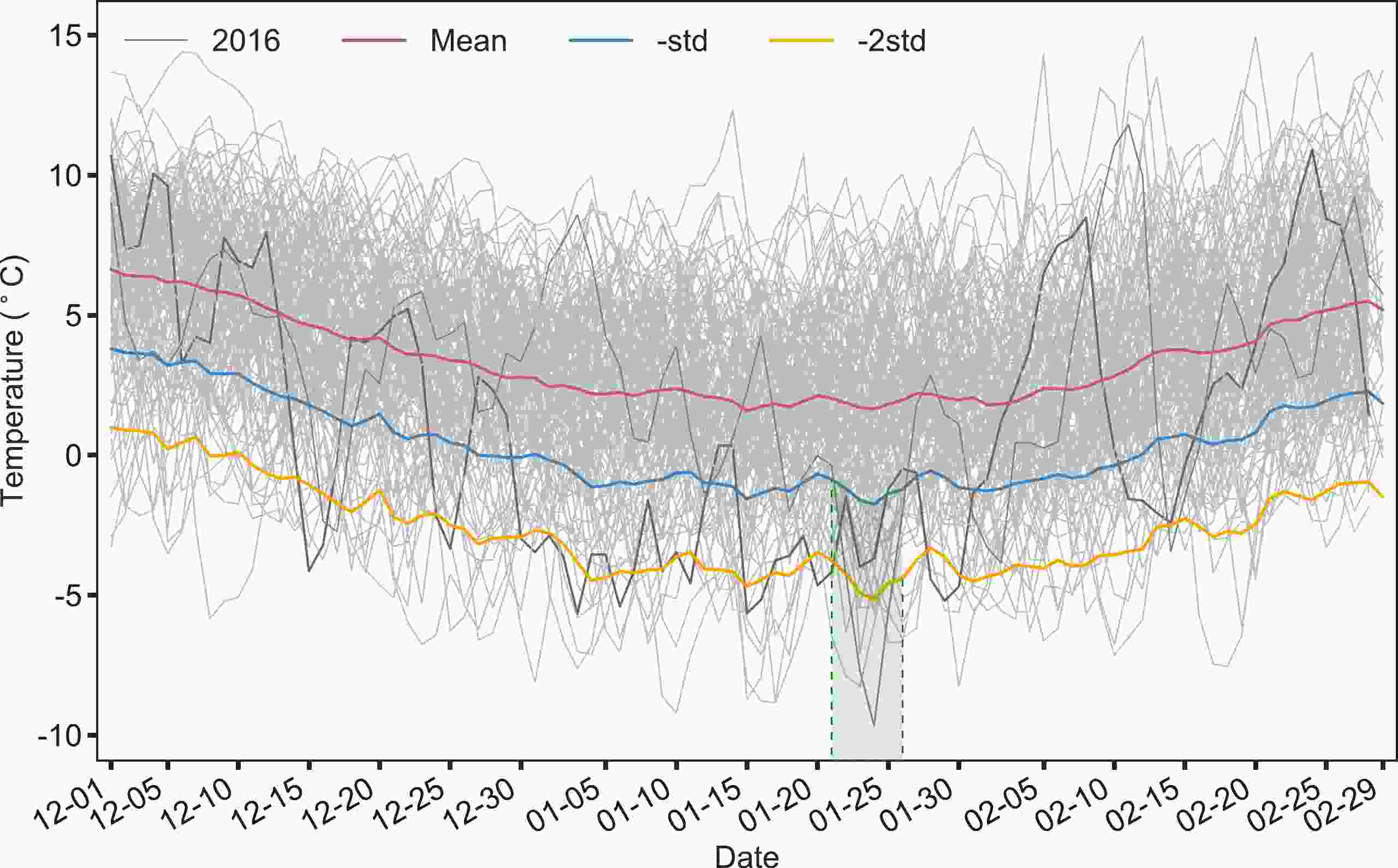
Figure 2. Daily temperature time series (gray lines) for southern China (22°–35°N, 107°–124°E) in winter (December, January, and February) during 1872–2017. The red line is the average time series. The blue line and yellow line are the temperatures less than one and two standard deviations, respectively. The black line is the temperature time series in 2016, and the green shading represents the timing of the “boss level” cold wave event.
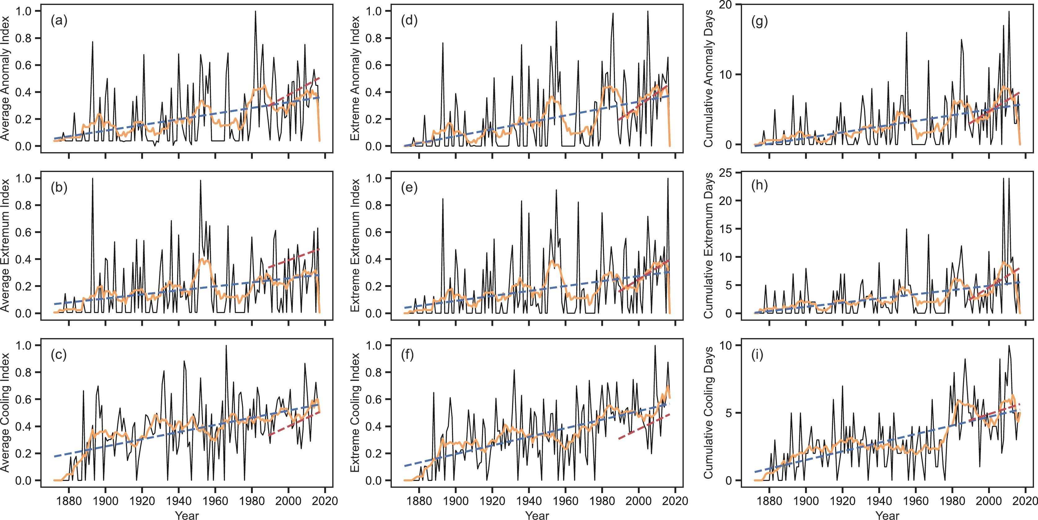
The annual time series were further analyzed using three methods: the first method is averaging the indices; the second method is calculating the extreme index values; and the third method is counting the cumulative days of ECWEs in each year. Thus, nine indices can indicate the intensity of the ECWEs in detail. They are average anomaly index (Fig. 3a), average extremum index (Fig. 3b), average cooling index (Fig. 3c), extreme anomaly index (Fig. 3d), extreme extremum index (Fig. 3e), extreme cooling index (Fig. 3f), cumulative anomaly days (Fig. 3g), cumulative extremum days (Fig. 3h), and cumulative cooling days (Fig. 3i). The results show significant increasing trends (blue lines) and decadal changes (orange lines) in all indices from 1872 to 2017. Their decadal variabilities suggest a larger increase after the late 1980s (red lines), indicating an increase in the intensity and frequency of ECWEs in southern China thereafter.
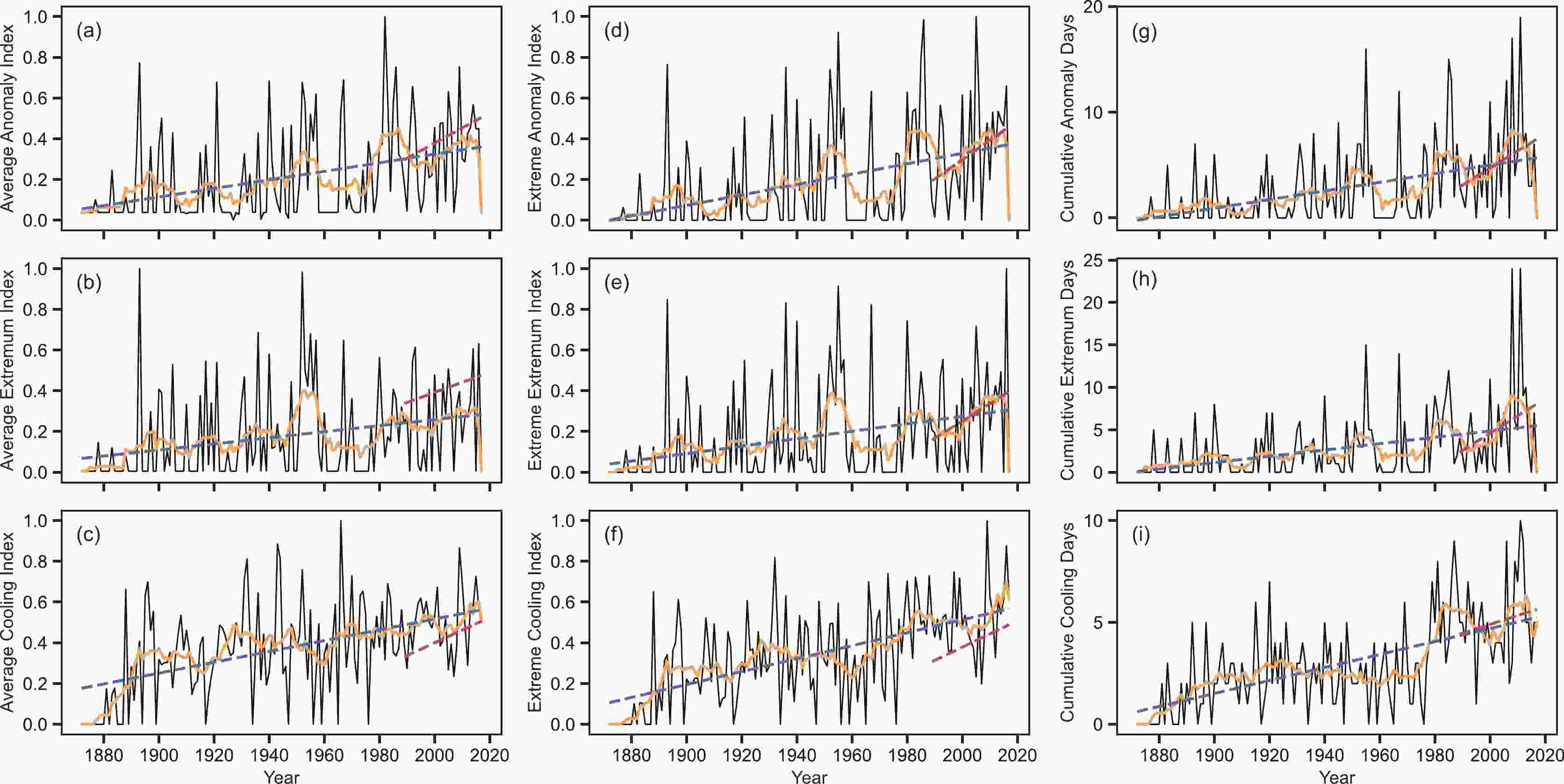
Figure 3. The annual (black line) and decadal (10-year running average, orange line) changes of the average anomaly, extremum, and cooling indices (a–c), extreme anomaly, extremum, and cooling indices (d–f), cumulative anomaly, extremum, and cooling days (g–i) during 1872–2017. The dotted lines represent the linear trend during 1872–2017 (blue) and after the late 1980s (red).
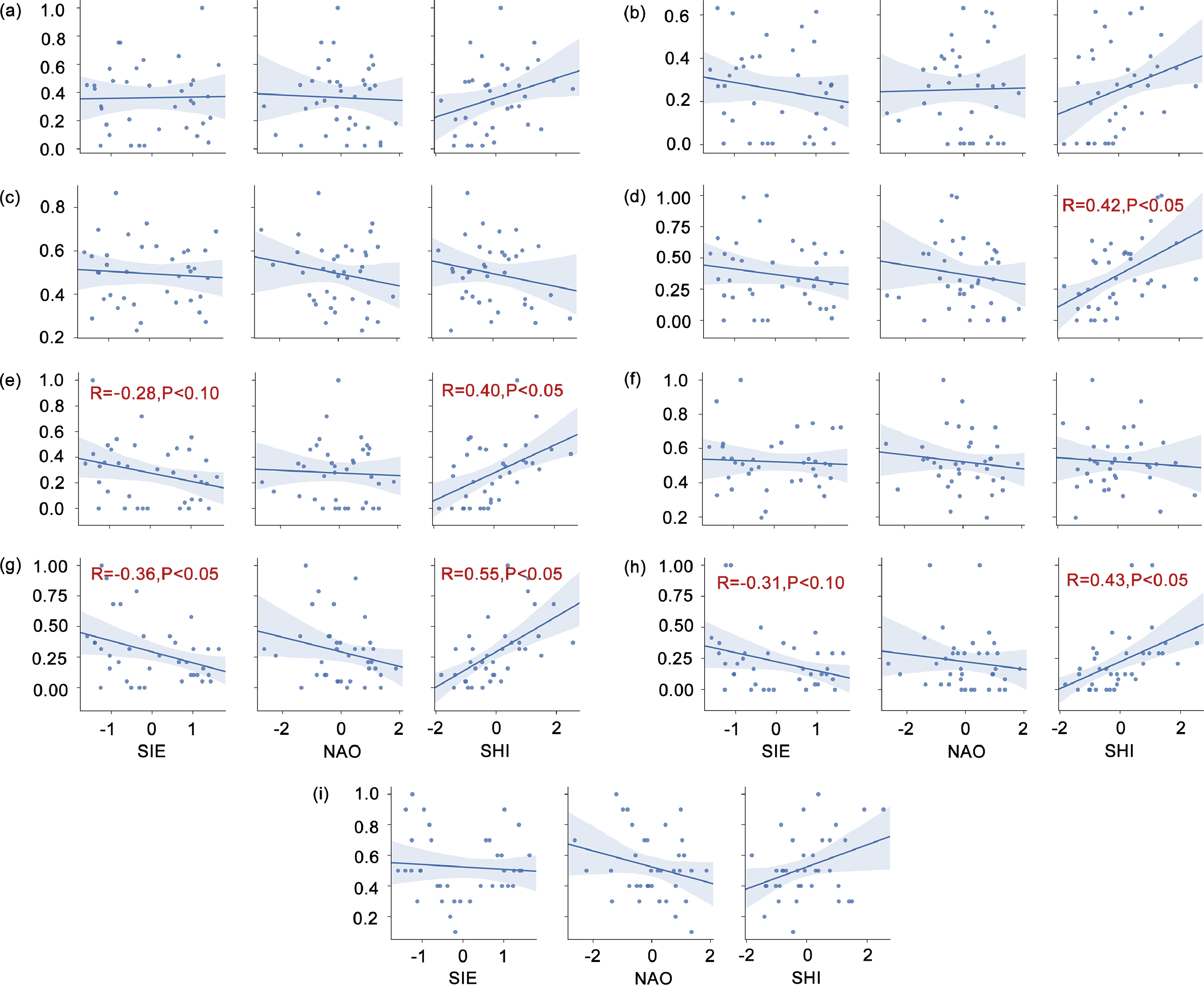
To investigate the relationship between the ECWEs, Arctic sea ice, and atmospheric circulation, the above ECWE indices were respectively analyzed against B–K SIE, the NAOI, and the SHI during 1981–2017 when sea ice satellite observations were available. As shown in Fig. 4, the average indices have no significant correlations with B–K SIE, the NAOI, or the SHI (Fig. 4a-c). The extreme anomaly index showed a positive correlation with the SHI (r = 0.42, at the 95% confidence level) (Fig. 4d). The extreme extremum index showed a negative correlation with SIE (r = –0.28, at the 90% confidence level) and a positive correlation with the SHI (r = 0.40, at the 95% confidence level) (Fig. 4e). The cumulative anomaly days showed a negative correlation with SIE (r = –0.36, at the 95% confidence level) and a positive correlation with the SHI (r = 0.55, at the 95% confidence level) (Fig. 4g). The cumulative extremum days showed a negative correlation with SIE (r = –0.31, at the 90% confidence level) and a positive correlation with the SHI (r = 0.43, at the 95% confidence level) (Fig. 4h).
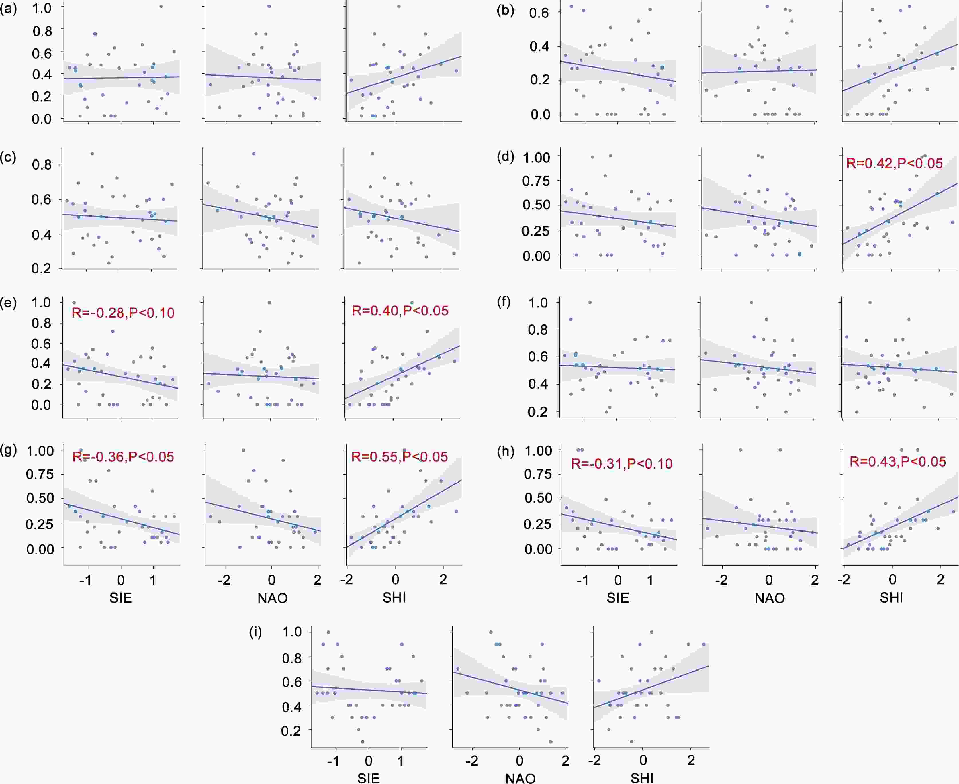
Figure 4. The correlations between the indices of ECWEs and autumn SIE in the B–K Seas, the winter NAOI, and the SHI during the period 1981–2017. (a), (b), and (c) represent the average anomaly index, average extremum index, and average cooling index, respectively; (d), (e), and (f) represent the extreme anomaly index, extreme extremum index, and extreme cooling index, respectively; (g), (h), and (i) represent the cumulative anomaly days, cumulative extremum days, and cumulative cooling days, respectively. The shaded bands indicate the 95% confidence interval.
The above results indicate that the extreme intensity and frequency of ECWEs are significantly correlated with the SIE of the B–K Seas and SH, while being slightly correlated with the average state of ECWEs. No significant correlations were found between the NAO and any of the indices. Due to the highest correlation being with both the SIE and the SHI, the cumulative anomaly days is normalized and further calculated as the Cold Index (CI) since it can characterize both the intensity and frequency of ECWEs.
-
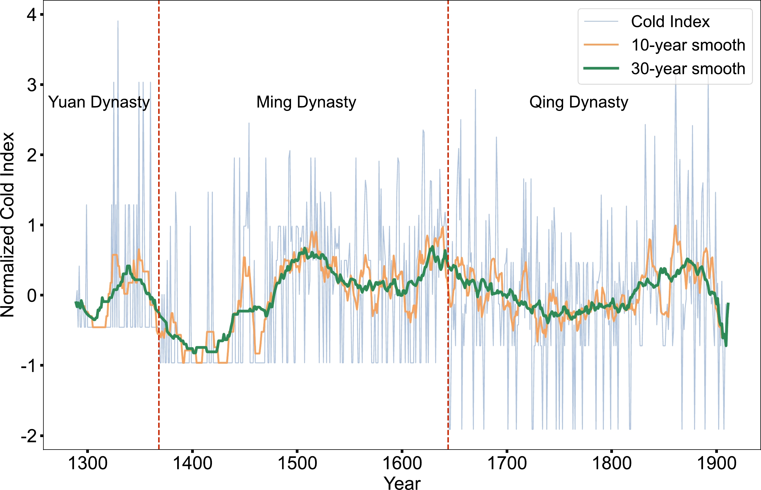
Based on the Chinese meteorological records of the past 3000 years, we further reconstructed the sequence of the CI from 1289 to 1911 (Fig. 5a). Due to the uneven temporal distribution of ancient records, there are considerable discrepancies in the record amounts of different time periods. For example, there are more records from the mid- to late- Ming dynasty to the Qing dynasty than from before the early Ming dynasty. It is therefore difficult to determine whether a period of relatively low CI is caused by a lack of records. To avoid the heterogeneity of temporal distribution, we assumed that the number of ancient records is constant in each dynasty, thus, the CI is subject to subsection normalization in accordance with the dynasty (Fig. 5b). A running average of 10 years and 30 years, respectively, for the CI (Fig. 6) showed four distinct cold periods between 1289–1911. These periods were the late Yuan dynasty (around the 1340s), mid-Ming dynasty (around the 1500s), late Ming and early Qing dynasty (around the 1640s), and late Qing dynasty (around the 1870s). This agrees well with previous studies (Table 1).
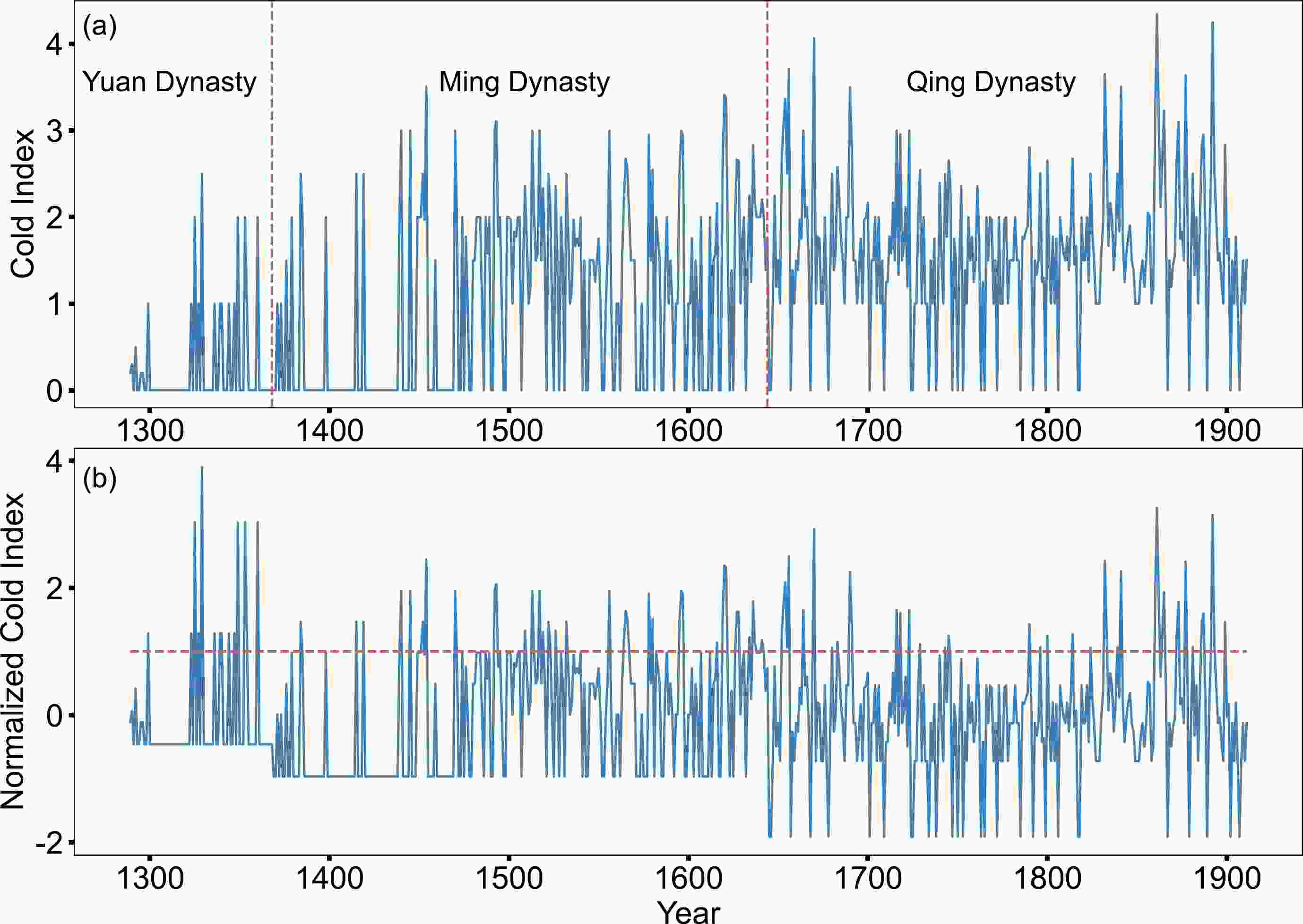
Figure 5. The reconstructed (a) and normalized (b) time series of the CI from 1289 to 1911. The red dotted lines in (a) are used to distinguish the Yuan, Ming, and Qing dynasties. The red dotted line in (b) represents one standard deviation.
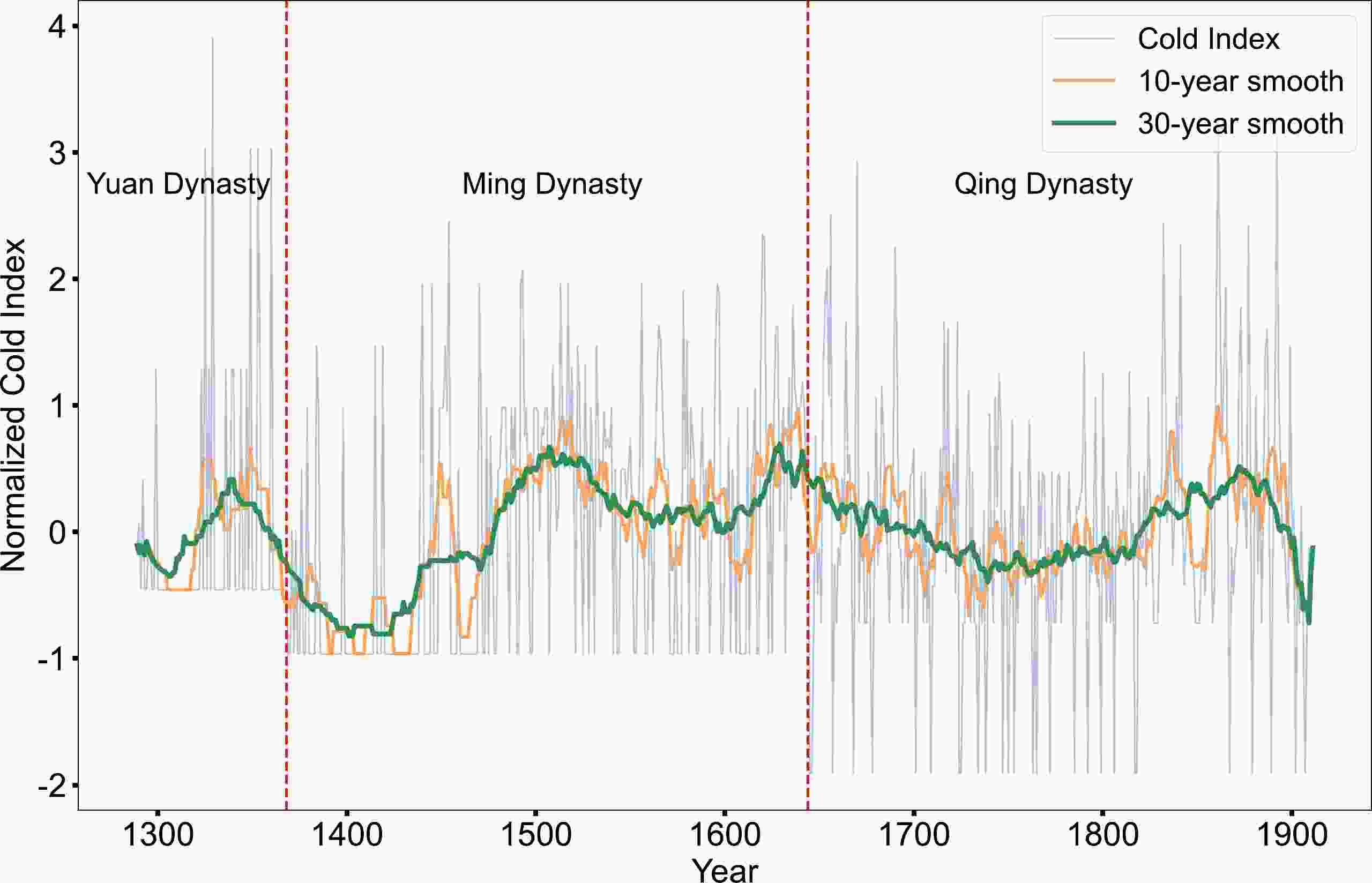
Figure 6. The annual (grey line), 10-year (orange line), and 30-year (green line) running average time series of the normalized CI from 1289–1911. The red dotted lines are used to distinguish the Yuan, Ming, and Qing dynasties.
Dynasty Cold Period 1 Cold Period 2 Reference Yuan 1320s−1340s − This Study 1300s−1390s − Wang et al.,1998 1320s-1340s − Ge et al., 2003 Ming 1480s−1520s 1620s−1644 This Study 1500−1520 1571−1644 Zhang, 1980 1470−1519 1550−1644 Wang and Wang, 1990 1491−1520 1621−1644 Zhao and Ye, 1996 1450s−1510s 1560s−1644 Wang et al., 1998 1430−1529 1610−1644 Chen and Shi, 2002 1411−1500 1500−1644 Ge et al., 2003 1490−1519 1620−1644 Han, 2003 Qing 1650s−1690s 1840s−1890s This Study 1640s−1690s 1831-1900 Zhang and Gong, 1979 1644−1690s 1790s−1890s Wang et al., 1998 1670−1710 1810−1840 Chen et al., 2005 1650−1699 1850−1899 Ge, 2011 Table 1. Reconstructed cold periods of Chinese Dynasties from 1289 to 1911.
Figure 6 shows that ECWEs occurred frequently and intensely during the 1320s–1340s, which has been previously identified as a typical cold period; Ge et al. (2003) took this period as a sign of the onset of the Little Ice Age in China. Then, in the early Ming dynasty, winters were warm and ECWEs occurred less frequently. Next, there was a strong cold wave frequency phase during the mid-15th century (from about the 1440s to the 1460s), which agrees with the results of Ge et al. (2003) that suggest a cold period during the 1440s–1470s. This was followed by two distinct cold periods during the 1480s–1520s and 1620s–1640s. The early and late Qing dynasty also included two distinct cold periods during the 1650s–1700s and 1860s–1890s, corresponding to the findings of other studies (see Table 1). However, there are some differences that may be related to the different objectives and purposes of each study. It should be noted that this study focuses on the intensity and frequency of ECWEs, while most previous studies have focused on the average temperature in winter.
-
Climate and weather events are phenomena on two different scales. But statistical explanations can be given for which extreme weather events tend to occur in which climate states. In the previous part of this study, a long time history of ECWEs is developed, and it is further analyzed in the following sections by addressing the question: Do ECWEs occur more or less frequently under certain climate states such as periods with high SIE or low SIE? The correlation analysis in section 3.1.1 suggests that the CI is significantly and negatively related to the autumn SIE in the B–K Seas during the instrumental period. This implies that when the autumn SIE was low, there were more frequent occurrences of ECWEs in southern China. This relationship during periods of different climatic backgrounds needs further investigation. In this section, we evaluate the frequency of ECWEs under high/low SIE for the whole study period (1289–2017), before (1289–1850) and after (1850–2017) the industrial revolution, and the period with rapid sea ice reduction (1981–2017). The CI record that covers the whole study period was segmentally standardized and spliced with the reconstructed CI from 1289 to 1911 and the instrumental-based CI from 1912 to 2017.
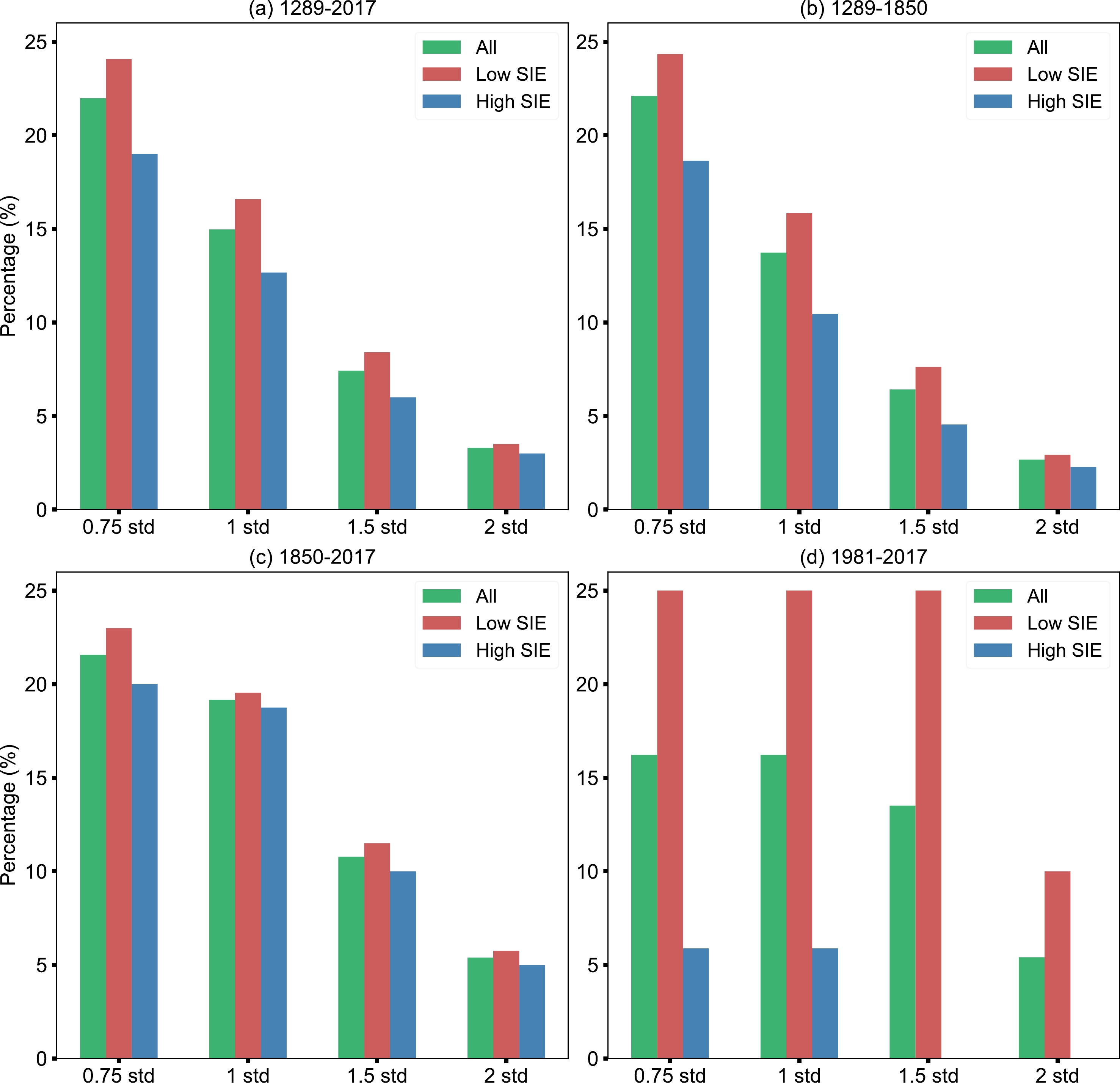
To quantify the frequency of ECWEs in the abnormally high or low SIE year, the reconstructed autumn SIE time series derived from Zhang et al. (2018b) was firstly normalized and detrended. The years with standardized SIE lower (higher) than 0 were defined as years of low (high) SIE. Meanwhile the anomalous strength of the CI is estimated using four criteria: the CI exceeding 0.75, 1, 1.5, and 2 standard deviations respectively. Accordingly, the proportion of strong cold winters occurring during the years of high or low SIE was determined. The results show that the proportion of strong cold winters occurring in low SIE years is higher than that in high SIE years (Fig. 7). Especially in the period from 1981 to 2017 (Fig. 7d), the proportions of strong cold winters of all four magnitudes are higher than the average for the whole study period (1289–2017) (Fig. 7a). In addition, all strong cold events above 1.5 and 2 standard deviations occur in the low SIE years. These results further show that the frequency of strong cold winters has increased since the 1850s, except for the 0.75-std magnitude (Fig. 7c), suggesting that the proportion of cold winters occurring in low SIE years has generally increased.
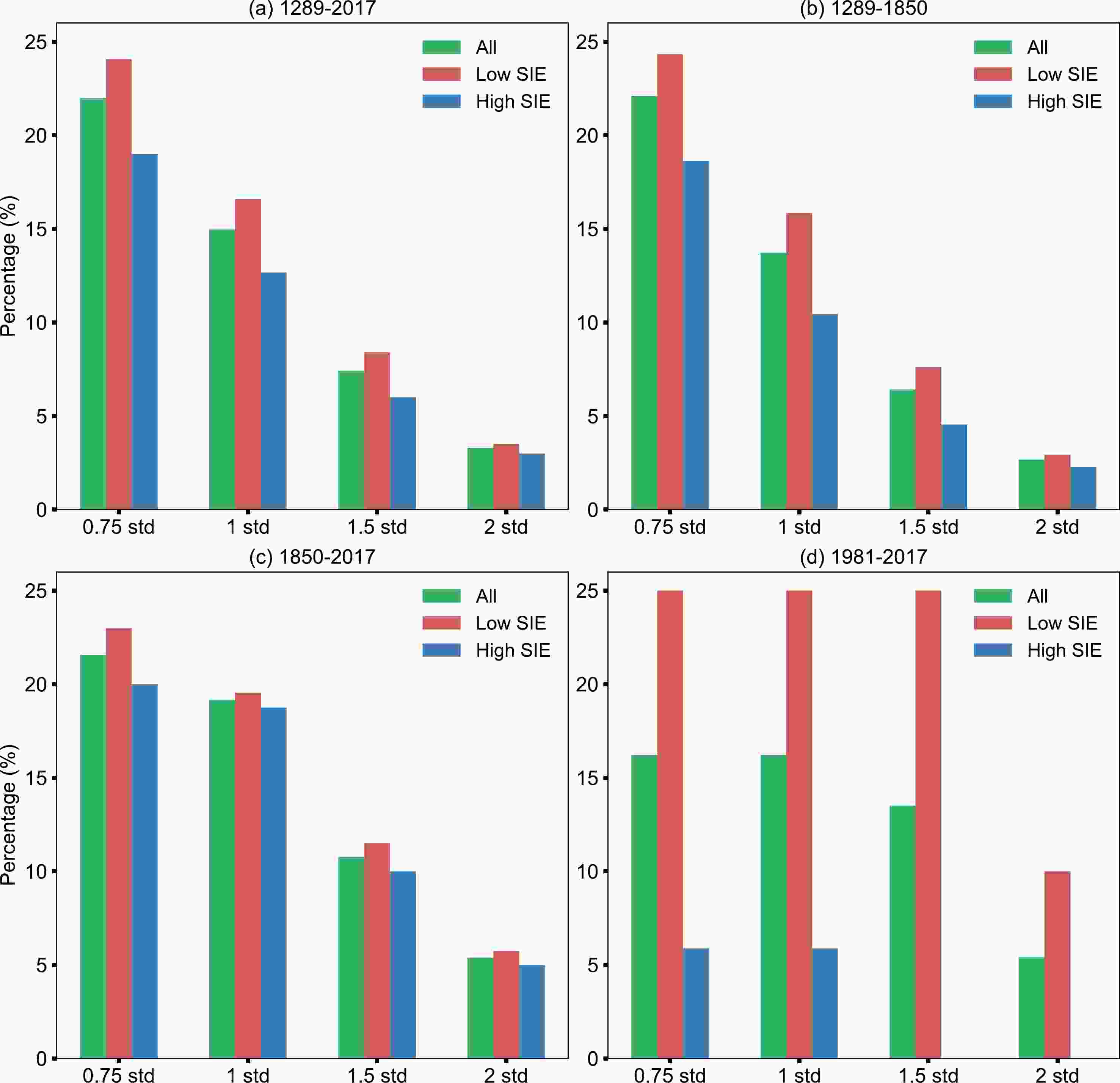
Figure 7. The proportion of ECWEs under high/low autumn SIE of the B–K Seas during 1289–2017 (a), 1289–1850 (b), 1850–2017 (c), and 1981–2017 (d).
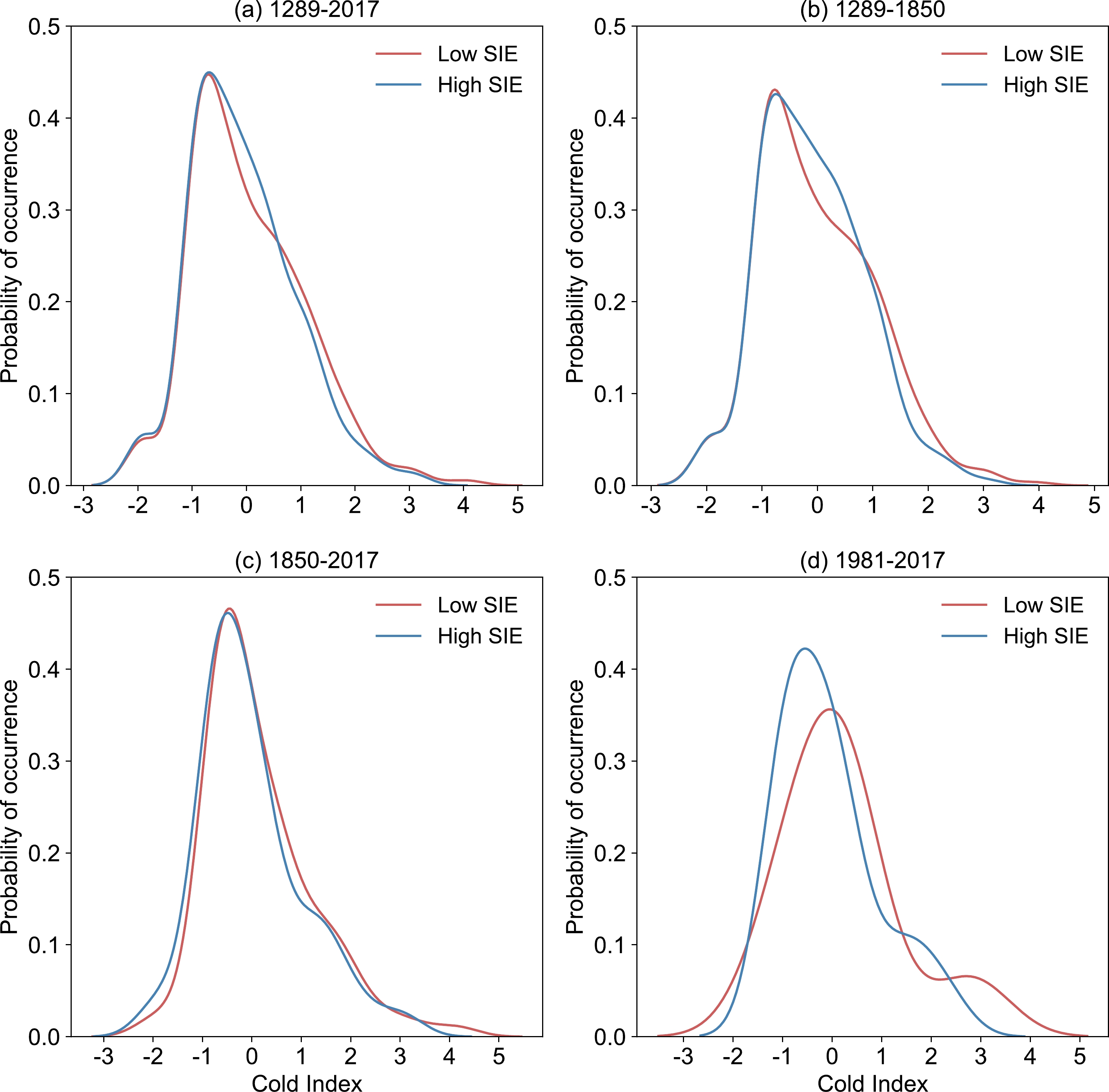
All probability density functions for the CI during four periods show their extreme cold tails shift to the right in response to low SIE compared to high SIE (Fig. 8). The shifts during 1289–2017 (Fig. 8a), 1289–1850 (Fig. 8b), and 1850–2017 (Fig. 8c) are weak, while the shift during 1981–2017 (Fig. 8d) is the most significant. The CI in low SIE years is, on average, 0.61 higher than in high SIE years during the period 1981–2017, 0.06 higher during the period 1850–2017, and showing no obvious change before 1850 and during the whole study period. Moreover, in low SIE years during 1981–2017, an increase in variability accompanied by a warm tail shift also leads to more warm events, which may be related to an increased interannual variability. These results imply an increase in the probability of extreme events, especially cold events, as well as an increase in the absolute value of the extremes’ response to low SIE in the continuous reduction period of SIE between 1981 to 2017.
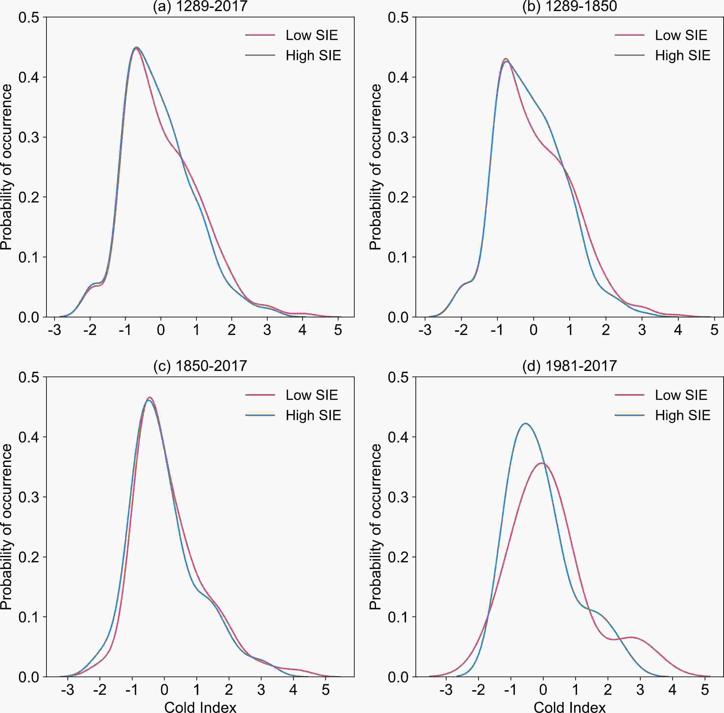
Figure 8. Probability density function of the CI under high/low autumn SIE in the B–K Seas during 1289–2017 (a), 1289–1850 (b), 1850–2017 (c), and 1981–2017 (d).
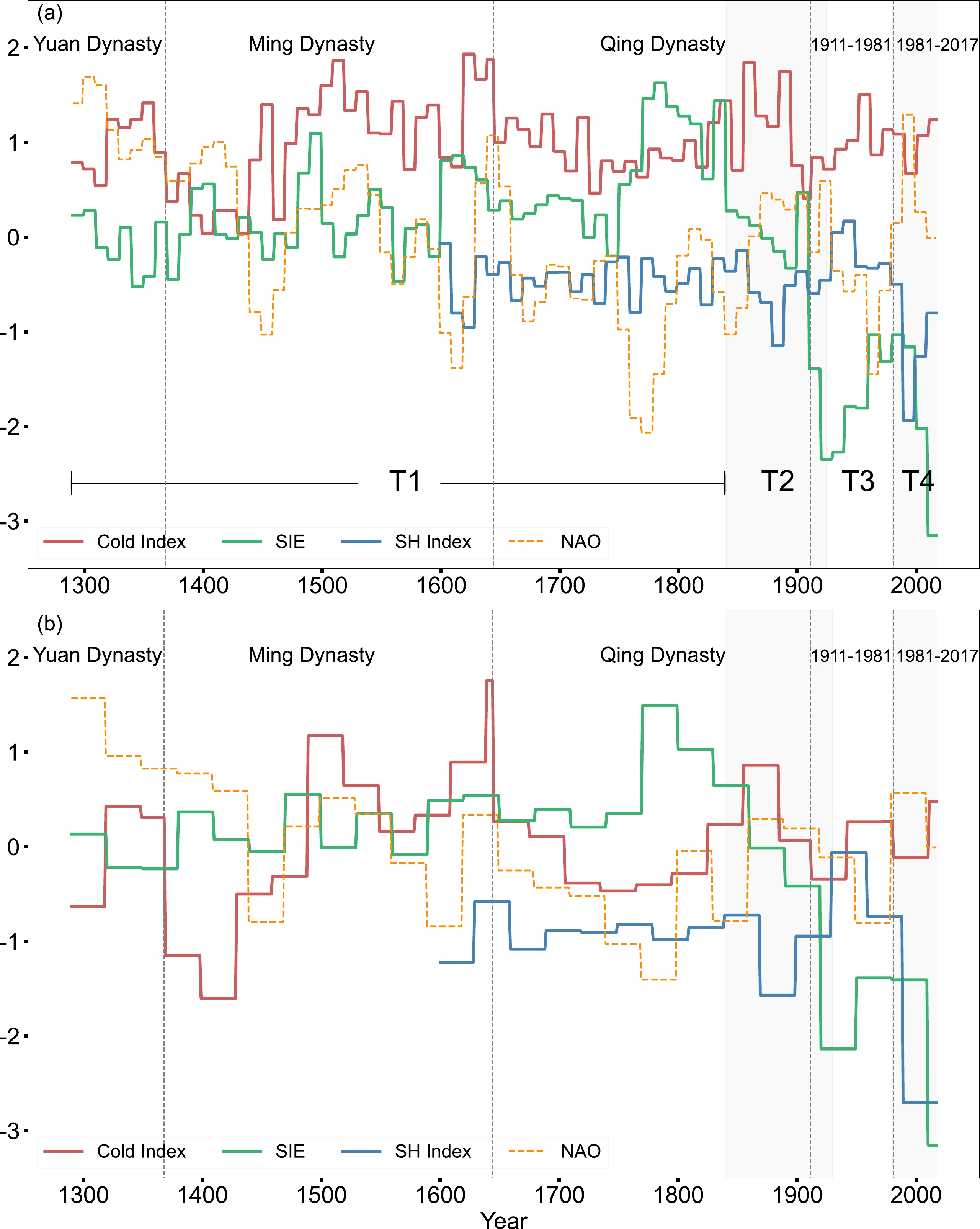
Figure 9 further shows that autumn SIE was negatively correlated with the CI in most periods, especially after the end of the 18th century. The periods with an out-of-phase relationship between SIE and the CI account for 71.4% of the 10-year average series (Fig. 9a). The above results confirm that sea ice melting in the Arctic is usually accompanied by a greater frequency of strong cold winters in southern China, suggesting that the substantial reduction of the B–K Seas SIE can explain, to some extent, the frequency of extreme cold winter events that have occurred in southern China in recent years. Next, we focus on the decadal changes of EWCEs in the context of different sea ice states and the possible linkage with the atmospheric circulation.
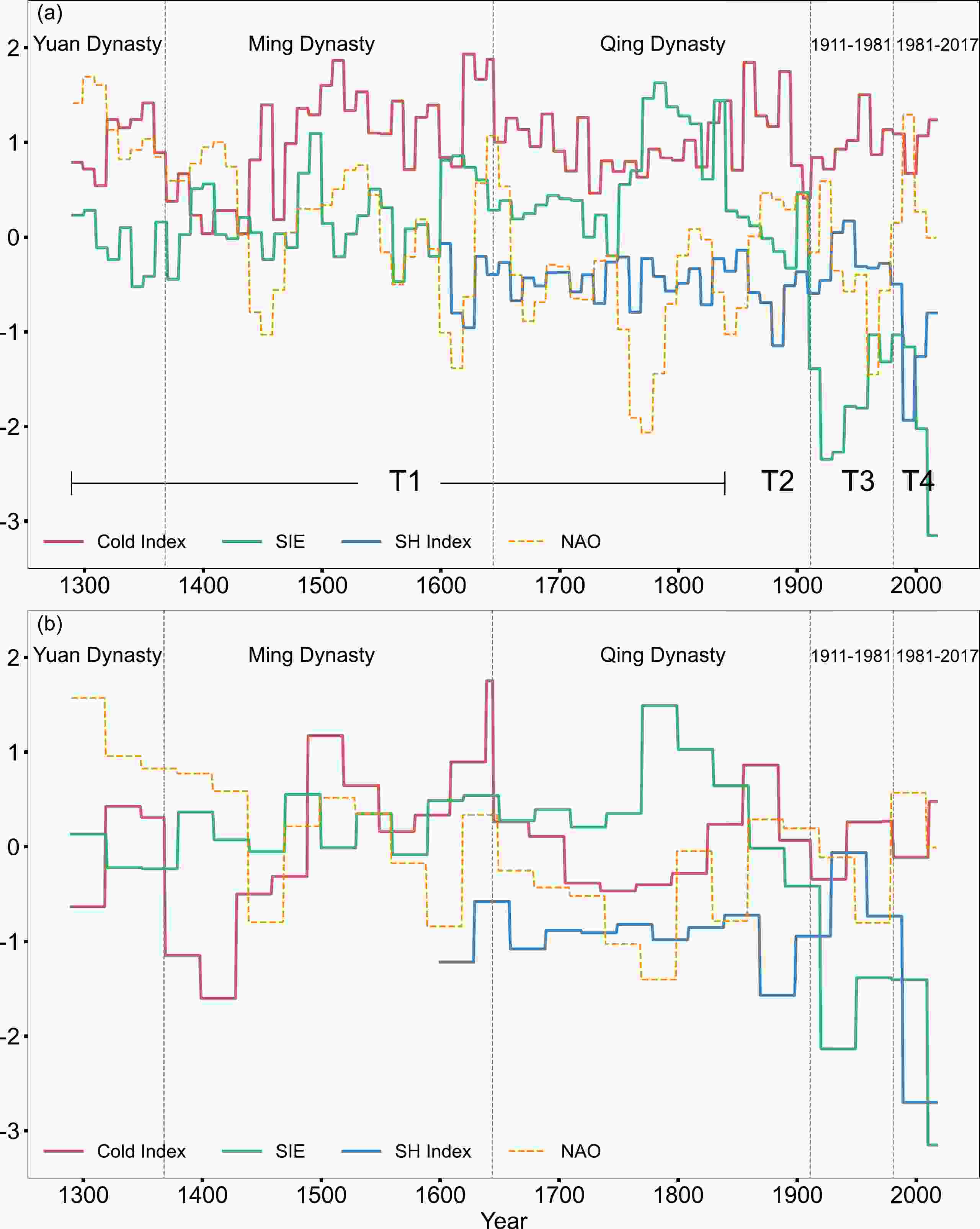
Figure 9. Time series of the 10-yr (a) and 30-yr (b) average CI, autumn B–K Seas SIE, the SHI, and the NAOI during 1289–2017.
-
Previous studies have suggested that the cooling in the midlatitudes is promoted by changes in atmospheric circulation involving a negative phase of the NAO and/or a strengthening of the SH (e.g., Deser et al., 2016; Chripko et al., 2021). The relationships between ECWEs, SIE, the NAOI, and the SHI during the instrumental period have been explored in section 3.1.1. The results suggest that the extreme intensity and the frequency of ECWEs are significantly correlated with the B–K Seas SIE and the SH but weakly correlated with the NAO on the interannual time scale. These relationships were further estimated combining the proxy-based reconstructions focusing on the context of different sea ice changes. According to the trends of SIE in the B–K Seas extracted from Zhang et al. (2018b), SIE change in the B–K Seas can be divided into four periods (Fig. 9a). In the T1 period from the late 13th century to the early 19th century, SIE is in a high-fluctuation state with a slight upward trend in the context of the Little Ice Age. From the 19th century onwards, the SIE enters a period of retreat (T2) and accelerates in the mid-19th century, afterwards reaching a trough around the 1930s, followed by a period of rebound (T3), but then entering another period of rapid retreat (T4) after the 1970s.
The results suggest that the relationships between the autumn SIE and the winter CI, NAOI, and SHI are not stable. Specifically, during the T4 period of rapid sea ice retreat, the CI shows a weak increasing trend and an in-phase change with the SH and an out-of-phase change with the NAO on the decadal time scale (Fig. 9). However, it seems more complex in the T2 period when the SIE continues to decrease before 1900 and the CI shows two extreme peaks accompanying the positive NAO and negative SH. After 1910, the SIE decreased at a greater rate, but the CI and SH showed a small upward trend; the NAO was in a positive phase. During the T3 period of SIE increase, the CI exhibited an increasing trend accompanied by a negative NAO and positive SH. During the T1 state before 1850, the SIE and the CI showed a roughly inverse variation. Meanwhile, we find that the negative correlation between SIE and the CI weakens during the expansion of SIE, such as in the late 14th and mid-late 17th centuries with a significantly negative NAO.
Our results suggest that the out-of-phase relationship between ECWEs and the B–K Seas SIE is unstable on the decadal time scale, even though it is investigated in the instrumental period. Meanwhile, the linkages with atmospheric circulation were also found to be unstable, which is in agreement with other recent studies (e.g., Xu et al., 2019; Dai and Song, 2020; Smith et al., 2022). During most periods with decreasing SIE, ECWEs occurred frequently and were probably contributed by a plausible atmospheric bridge between the midlatitudes and the Arctic. The percentage of ECWEs happening in low SIE periods is much higher than that in high SIE periods, especially during 1981–2017. However, in the periods with more ECWEs, the B–K Seas SIE is not always at a low level. It is inferred that in these cases the atmospheric bridge is probably destroyed due to the internal atmospheric variability on the decadal time scale (Sung et al., 2018; Xu et al., 2019). It is likely that the internal variability of the atmospheric circulation weakened the influence of sea ice because a strong NAO (weak SH) is not conducive to cold air being transported southward (Zheng et al., 2022). In addition, recent studies have reported that the stratospheric internal variability is associated with large uncertainty in the tropospheric circulation response to sea ice loss and can completely obscure the forced NAO circulation response and associated impacts on air temperatures over the midlatitudes (Smith et al., 2022; Sun et al., 2022).
-
In this paper we have investigated the statistical relationship between autumn sea ice changes in the B–K Seas and winter ECWEs in southern China based on observed and reconstructed data of SIE and the CI from 1289 to 2017. A strong anti-phase relationship between autumn B–K Seas SIE and the winter CI was found during the instrumental period (1981–2017). Autumn B–K Seas SIE has experienced a rapidly decreasing trend and winter extreme cold events have occurred frequently in recent years. Before that, the relationship was not stable and showed a strong correlation in the low-SIE period and a weak correlation in the high-SIE period. The evaluation of the frequency of ECWEs in different periods shows ECWEs shifting toward being more frequent and more serious in low-SIE years compared to high-SIE years. This response to low SIE was amplified, especially in the continuous reduction period of SIE between 1981 to 2017. Some studies have identified an influence mechanism linking Arctic sea ice to cold wave events in Eurasia and east Asia through the “bridge” role of atmospheric circulation associated with the NAO and SH. Through comparing SIE, the CI, the NAOI, and the SHI, we found that the atmospheric bridge was not always stable either.
During most periods of autumn B–K Seas sea ice melting, the SIE showed an anti-phase correlation with both the SHI and CI, and an in-phase correlation with the NAO. The negative trend in the NAO over the past two decades has been linked to the reduction of sea ice in the B–K Seas (Cohen et al., 2012; Nakamura et al., 2015; Yang et al., 2016). Reduction of Arctic SIE can also significantly strengthen and reinforce the presence of the SH (Wu and Wang, 2002; Wu et al., 2011). The circulation changes over the Ural–Siberian region are also suggested to provide a link between B–K Seas sea ice and the NAO (Santolaria-Otín et al., 2020). Optimal circulation, such as Ural Blocking concurring with the positive phase of the NAO, can favor the intrusion of midlatitude North Atlantic moisture and water vapor into the B–K Seas region (Luo et al., 2017). A negative NAO and a strengthened SH are conducive to storm tracks shifting equatorward and cold air moving southward, directly resulting in frequent winter extreme cold events across Eurasia (Herring et al., 2016; Whan et al., 2016; Yao et al., 2016; Martineau et al., 2017; Zheng et al., 2022). In addition, recent studies have revealed that the “stratospheric pathway” may play an important role in the atmospheric circulation response to observed sea ice loss in the B–K Seas (Nakamura et al., 2016; Wu and Smith, 2016; Zhang et al., 2018a, b). It is suggested that a weakening of the stratospheric polar vortex (Kretschmer et al., 2020) and its increased variability (Kretschmer et al., 2016) related to the enhanced sea ice loss in the B-K Seas would induce a negative NAO, the warm Arctic–cold continents pattern (Kim et al., 2014), and an increase in cold-air outbreaks in the midlatitudes (Kretschmer et al., 2018). Therefore, the “bridge” role of atmospheric circulation is supported by the above mechanism during the lower autumn B–K Seas SIE period.
However, ECWEs do not always occur during low-SIE periods. When SIE expands in the B–K Seas, more ECWEs will also occur if the NAO is in a strong negative phase on the decadal time scale. There is observational evidence that a strong negative NAO can lead to more cold winters in East Asia on the multidecadal time scale via the ocean–atmospheric bridge mechanism (Xie et al., 2019; Li et al., 2022). The modulation of a strong NAO likely weakens the negative relationship between SIE and the CI. The strength of the Arctic–midlatitude linkage on the decadal time scale is inferred to be associated with the internal atmospheric variability. This is supported by recent multimodel simulations that suggest the internal variability in the polar stratosphere may be a source of noise that increases the uncertainty in the response of tropospheric atmospheric circulation to Arctic sea ice loss (Peings et al., 2021; Smith et al., 2022; Sun et al., 2022).
This study implies that the effect of autumn B–K Seas SIE on extreme winter cold events in southern China is more significant when SIE retreats. The contribution by sea ice would be partially offset by the atmospheric internal variability when SIE expands. Palaeoclimate data helps to overcome known limitations in observations and model simulations of the influence of the Arctic on midlatitude climate and demonstrates that the linkages might change between different climate contexts. The results may be influenced by the inevitable uncertainty associated with the limited data used for the reconstructions. The extension of quantitative proxy-based records with enough accuracy and comparisons with climate models are needed to provide enough evidence to understand the mechanism and draw robust conclusions in the future.
Acknowledgements. This research was supported by the National Natural Science Foundation of China (Grant No. 42101142), the Strategic Priority Research Program of the Chinese Academy of Sciences (Grant No. XDA19070103) and the Young Elite Scientists Sponsorship Program by CAST (Grant No. 2022QNRC001).
| Dynasty | Cold Period 1 | Cold Period 2 | Reference |
| Yuan | 1320s−1340s | − | This Study |
| 1300s−1390s | − | Wang et al.,1998 | |
| 1320s-1340s | − | Ge et al., 2003 | |
| Ming | 1480s−1520s | 1620s−1644 | This Study |
| 1500−1520 | 1571−1644 | Zhang, 1980 | |
| 1470−1519 | 1550−1644 | Wang and Wang, 1990 | |
| 1491−1520 | 1621−1644 | Zhao and Ye, 1996 | |
| 1450s−1510s | 1560s−1644 | Wang et al., 1998 | |
| 1430−1529 | 1610−1644 | Chen and Shi, 2002 | |
| 1411−1500 | 1500−1644 | Ge et al., 2003 | |
| 1490−1519 | 1620−1644 | Han, 2003 | |
| Qing | 1650s−1690s | 1840s−1890s | This Study |
| 1640s−1690s | 1831-1900 | Zhang and Gong, 1979 | |
| 1644−1690s | 1790s−1890s | Wang et al., 1998 | |
| 1670−1710 | 1810−1840 | Chen et al., 2005 | |
| 1650−1699 | 1850−1899 | Ge, 2011 |


 AAS Website
 AAS WeChat