Improved Microwave Ocean Emissivity and Reflectivity Models Derived from Two-Scale Roughness Theory

Space-borne microwave polarimetric measurements have been widely used for the remote sensing of surface and atmospheric parameters. In passive ocean remote sensing, an accurate radiative transfer model is normally required to simulate the radiance emanating from the Earth’s atmosphere (He et al., 2010; Mech et al., 2020). In the microwave region, the downwelled atmospheric radiation to oceanic surfaces is either absorbed or reflected. In solving the radiative transfer equation, the ocean emission and reflection terms are expressed as the lower boundary conditions, and their uncertainties critically affect the simulation accuracy. Therefore, accurate microwave ocean surface reflection and emission models are required to better understand the variables affecting the oceanic radiative transfer process and help retrieve its surface geophysical parameters from satellite measurements (Jin et al., 2021).

In the past, many studies were devoted to developing ocean emissivity models. The Laboratoire d'Océanographie et du Climat (LOCEAN) is a physical model fine-tuned to the L-band (Dinnat et al., 2003; Yin et al., 2016). It is derived from the two-scale model of Yueh (1997). The FAST Emissivity Model (FASTEM) is a fast-linear regression fit to the output of a physical two-scale model (English and Hewison, 1998; Liu et al., 2011) commonly used for the numerical assimilation of satellite data. This model is only suitable for frequencies 6–200 GHz. Remote Sensing Systems (RSS) also developed an empirical model fine-fitted to satellite observations (Meissner and Wentz, 2004, 2012). The well-known two-scale roughness theory is widely used to develop the physical microwave ocean surface emissivity model (Wu and Fung, 1972; Wentz, 1975; Yueh, 1997; Germain et al., 1998; Johnson, 2006). The reflection contribution of the ocean surface to upwelling radiance is always simulated by the Geometrical Optics (GO) model, which considers the ocean surface as an ensemble of facets having different slopes (Fan et al., 2010; He et al., 2010). The GO model is known to be less accurate at low frequencies and large zenith angles. A small perturbation method (SPM), which assumed a random rough ocean surface without sea foam, was used to derive the reflectivity matrix for radiative transfer applications (Zhang et al., 2002). Recently, a full reflectivity matrix was derived from the two-scale theory for the vector radiative transfer but the dielectric model is only applicable for frequencies lower than 10 GHz (Jin et al., 2021).

The fast radiative transfer models such as the Community Radiative Transfer Model (CRTM) (Weng and Liu, 2003; Weng, 2007), the Radiative Transfer for TOVS (RTTOV) (Saunders et al., 1999, 2018), and ARMS (Weng et al., 2020) are developed for satellite data assimilation. In these models, the FASTEM is used to calculate the emissivity vector and the reflectivity vector is then derived from the emissivity vector using polarimetric Kirchhoff’s law. Kilic et al. (2019) evaluated three ocean RTMs based on the RTTOV, and the reflection terms of the ocean surface were estimated by means of coefficient correction. Jin et al. (2021) developed a comprehensive vector radiative transfer model for estimating salinity. The reflectivity matrix for the L band was developed, but the emissivity was calculated from a semiempirical model. Presently, the two-scale roughness theory is not well explored for simultaneously computing the emissivity vector and reflectivity matrix in coupled atmosphere-ocean radiative transfer models.

Many previous studies have proven that the two-scale theory performs well in simulating the surface scattering and emission from ocean surfaces (Yueh et al., 1994; Pierdicca et al., 2000; Dinnat et al., 2002; Lyzenga and Vesecky, 2002; Johnson et al., 2004; Bettenhausen et al., 2006). The theory simulates the ocean surface as large-scale gravity waves and small-scale capillary waves, with the small-scale waves riding on top of the large-scale waves. The scattering from the small-scale waves is called Bragg scattering and can be calculated up to the second order based on the SPM, whereas the scattering from the large-scale waves can be simulated as slightly perturbed surface patches using the GO model. Small-scale waves contribute in two main ways to ocean surface reflection. The first is the first-order bistatic incoherent scattering, and the second is the second-order coherent scattering similar to specular reflection. Large-scale waves have a tilting effect and depolarize the incident radiation. The two-scale theory combines the advantages of the SPM and GO models, allowing these scattering and emission models based on this theory to be applied over a wider range of frequencies, observation angles, and wind speeds. The purpose of this study is to develop physical reflectivity and emissivity models from two-scale roughness theory. The two models are suitable for a wide range of microwave frequencies at various observation angles and environmental conditions and will be used as lower boundary conditions of the vector radiative transfer model for passive remote sensing of the ocean surface. In section 2, the two-scale roughness theory are briefly described, and the full expressions of the ocean surface reflectivity matrix and emissivity are demonstrated from the two-scale roughness theory. Section 3 describes the dependences of the reflectivity matrix and emissivity on the zenith angle, azimuth angle, frequency, and the wind vector. Moreover, the upwelling BT, as contributed from ocean emission and reflections are calculated from two-scale reflectivity model (TSRM) and two-scale emissivity model (TSEM) and compared with those from GO and FASTEM. The summary and conclusions are given in section 4.

Two-scale roughness theory is comprised of five components, the ocean water dielectric constant model, sea-surface roughness model, hydrodynamic modulation model, cutoff wavenumber model, and foam model.

In microwave ocean remote sensing, the dielectric constant is an important physical parameter that affects the reflection and emission of the ocean surface. It is generally obtained by fitting the laboratory data as a function of frequency, salinity, and temperature and can be divided into single Debye models (Debye, 1929; Klein and Swift, 1977) and double Debye models (Liebe et al., 1991; Guillou et al., 1998; Meissner and Wentz, 2004). The single Debye model is a good approximation for pure water and seawater at low microwave frequencies. When the frequencies are higher than 10 GHz, the accuracy of single Debye models decreases. Because this study is geared to develop a reflectivity matrix and emissivity model with a wide frequency range, a double Debye dielectric model (Liu et al., 2011) is adopted and can be applied to a frequency range of 1.4 to 410 GHz and a temperature range of –2°C to 30°C.

The modified Durden and Vesecky (DV) ocean surface wavenumber spectrum is used as part of the two-scale model. The large-scale slope derived from the DV model is adjusted for the underestimated Cox and Munk slope variance (Donelan and Pierson, 1987), which makes the theoretical results more consistent with experimental data (Yueh, 1997). The DV spectrum is empirical and valid over a large range (0°–70°) of incidence angles (Durden and Vesecky, 1985). It must be mentioned that the roughness model in this study only depends on the wind and is not a function of other factors (i.e., rainfall and boundary stability). The hydrodynamic effect modulates the distribution of short waves in the wind direction and makes the short waves more concentrated on the leeward sides of large-scale waves and therefore causes the asymmetry between upwind and downwind locations.

Ocean foam can be simulated as a layer of spherical water bubbles. In high winds, air is entrained into the water layer, and the air bubbles in the water modifies the water dielectric constant, affecting the scattering properties of the ocean surface. The contribution of foam on reflection should consider not only foam reflectivity but also foam coverage. Due to the lack of a rigorous and theoretical full-polarimetric reflectivity model for foam, Stogryn’s (2003) empirical reflectivity model and the empirical foam coverage function of Monahan and O’Muircheartaigh (1986) are used to calculate the reflection contribution of foam.

The cutoff wavenumber is a key parameter that distinguishes between the large-scale and small-scale waves and makes the root-mean-square height of the small-scale wave valid for the SPM and the curvature of the large-scale waves fit for the GO. Compared with the emissivity calculation, the cutoff wavenumber selection has a greater impact on the reflectivity. The cutoff wavenumber scheme requires a frequency dependence, as reflection and emission models must be suitable for a wider frequency range. Therefore, the Guissad and Sobieski scheme (Liu et al., 2011) is selected, which includes a function of frequency and wind speed.

In general, the reflected electric field of a rough surface can be expressed as:

where $i = \sqrt { - 1} $; $k$ is the wavenumber; $r$ is the distance of the scattering field from the incident field; the superscripts $i$ and $s$ stand for incident and scattering field, and the subscripts ν and $h$ represent vertically and horizontally polarized waves, respectively. Horizontal polarization is in the reflection plane, and vertical polarization is orthogonal to the reflection plane. The 2 × 2 amplitude scattering matrix $ {\mathbf{S}} $ relates the incident field $ {{\mathbf{E}}^i} $ to the reflected electric field $ {{\mathbf{E}}^s} $.

In most cases, the Stokes vector $ {\mathbf{I}} = \left( {I,Q,U,V} \right) $ is used in vector radiative transfer simulations. The first Stokes parameter $ I $ describes the total intensity of a beam of electromagnetic radiation, $ Q $ and $ U $ represent the linearly polarized component, and $ V $ represents the circularly polarized component. But the surface radiation is often expressed in terms of a modified Stokes vector $ {\mathbf{I}} = \left( {{I_v},{I_h},U,V} \right) $ for the convenience of various applications. The reflectivity matrix and emissivity vector transform into the corresponding forms before participating in the radiative transfer simulation. The relationship between the modified Stokes vector and the electric vector is defined as follows:

where Re and Im represent the real and imaginary parts of a complex number. The asterisk represents the complex conjugate. $ {I_v} $ and $ {I_h} $ are the radiance of vertical and horizontal polarizations, $ U $ and $ V $ characterize the correlations between these two polarizations, and the angular brackets denote the ensemble average of the argument.

For the electromagnetic-wave scattering from an ocean surface, a 4 × 4 reflection coefficient matrix $ {\mathbf{R}} $ is also commonly used, which relates the scattered Stokes vector to the incident Stokes vector. The elements in the reflection coefficient matrix can be derived from the amplitude scattering matrix (Perrin, 1942; Van de Hulst, 1957). The scattered Stokes vector $ {{\mathbf{I}}^s} $ is related to the incident Stokes vector $ {{\mathbf{I}}^i} $ by the reflection coefficient matrix as follows:

Through the application of Eqs. (1–4) $ {\mathbf{R}} $ can be expressed in terms of the amplitude scattering matrix $ {\mathbf{S}} $, as in Eq. (5), where Re and Im represent the real and imaginary parts of a complex number, respectively. It follows:

This section describes the derivation of the 4 × 4 reflection coefficient matrix $ {\mathbf{R}} $ from the amplitude scattering coefficients $ {S_{\alpha \beta }} $ ($ \alpha ,\beta = v,h $). The derivation of the two-scale reflectivity matrix $ {\mathbf{A}} $ requires the reflection coefficient matrix.

The two-scale theory simulates the reflectivity matrix $ {\mathbf{A}} $ contributed by the large-scale waves through the GO and the small-scale reflection through the SPM. The large-scale contribution is a coherent term and comes from facets whose orientations make specular reflections. The small-scale contribution includes both the first-order bistatic incoherent scattering (SPM1) and the second-order coherent scattering (SPM2). The SPM2 is similar to the large-scale that only occurs in the specular direction, while SPM1 is an average result over the large-scale surface slopes because a tilted facet scatters the radiation into all directions. Because the SPM2 and large-scale scattering have the same characteristics, these two parts can be combined into one coherent term. Thus, the total reflectivity matrix $ {\mathbf{A}} $ can be expressed as follows:

To derive the coherent and incoherent reflectivity matrices, first, we need to obtain the coherent and incoherent reflection coefficient matrices based on the theory in section 2.2.

For the coherent scattering, the amplitude scattering matrix is given as follows:

where $ {S_{vv}} $ and $ {S_{hh}} $ are the Fresnel reflection coefficients. $ S_{\alpha \beta }^{(2)} $ ($ \alpha ,\beta = v,h $) are the second-order reflection coefficients of SPM (Yueh et al., 1994).

The amplitude scattering matrix of incoherent scattering is expressed as

where $ S_{\alpha \beta }^{(1)} $ ($ \alpha ,\beta = v,h $) are the first-order reflection coefficients of SPM (Yueh et al., 1994).

Using Eqs. (5, 7, and 8), we can obtain the coherent reflection coefficient matrix $ {{\mathbf{R}}_{co}} $ and incoherent reflection coefficient matrix $ {{\mathbf{R}}_{inco}} $. Due to the incoherence of $ {{\mathbf{R}}_{inco}} $, it will be averaged over the slope distribution of Cox and Munk (Jin et al., 2021).

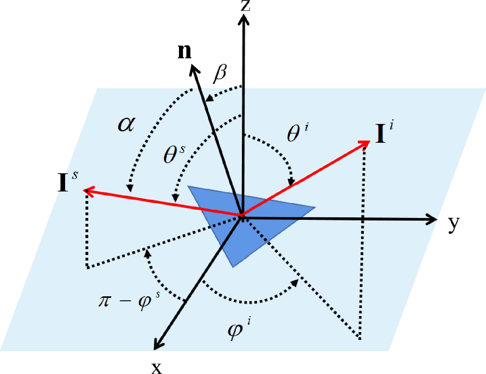
The reflection coefficient matrices $ {{\mathbf{R}}_{co}} $ and $ {{\mathbf{R}}_{inco}} $ are in a local coordinate system that is based on the facets. As shown in Fig. 1, the deep blue area represents the large-scale facet. The local coordinate system is established based on a facet, and n is the facet normal. $ {{\mathbf{R}}_{co}} $ and $ {{\mathbf{R}}_{inco}} $ are calculated in the local coordinate system but must be transformed to an Earth coordinate system before involving reflectivity matrix calculations.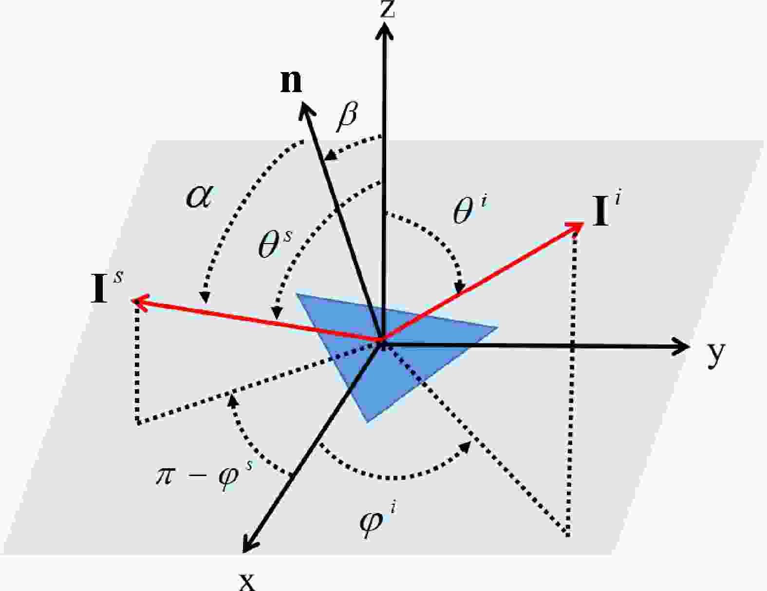

Figure 1.  Scattering geometry of a single tilted facet. $ {{\mathbf{I}}^i} $ is the incoming radiance vector incident from the $ ({\theta _i},{\varphi _i}) $ direction of a facet (deep blue area). $ {{\mathbf{I}}^s} $ is the outgoing radiance vector in the $ ({\theta _s},{\varphi _s}) $ direction. The angle $ \beta $ is the polar angle from the mean surface normal $ z $ to the facet-normal n. The angle $ \alpha $ is the incident angle and reflected angle with respect to facet normal.

where $ ({\theta ^{il}},{\varphi ^{il}};{\theta ^{sl}},{\varphi ^{sl}}) $ is a local geometry, $ ({\theta ^i},{\varphi ^i};{\theta ^s},{\varphi ^s}) $is a global geometry in the earth coordinate system. When deriving the reflectivity matrix, we first convert a global geometry to a local geometry to calculate the reflection coefficient matrices, then rotate the reflection coefficient matrices from the local geometry to the global coordinate system. $ P({Z_x},{Z_y}) $ is the Cox and Munk probability density distribution function; $ {Z_x} $ and $ {Z_y} $ represent the surface slopes in upwind (Fig. 1 along the x-axis) and crosswind (Fig. 1 along the y-axis) directions, respectively. $Z'_x$ and $Z'_y$ represent the surface slopes along and across the scattering azimuthal directions (Fig. 1 azimuth angle direction of $ {{\mathbf{I}}^s} $), respectively. $ \Gamma $ is the shadow function. $ \beta $ is the cosine of the polar angle from the mean surface normal to the facet normal. $ {k_0} $ is the free-space electromagnetic wavenumber. $ {W_s} $ is the small-scale part of an ocean surface spectrum, $ h $ is a hydrodynamic parameter, $ {i_1} $ is the rotation angle between the incident plane and the scattering plane, and $ {i_2} $ is the rotation angle between the outgoing plane and the scattering plane. $ {\mathbf{L}} $ is the rotation matrix. For modified Stokes vector $ \left( {{I_v},{I_h},U,V} \right) $ , $ {\mathbf{L}} $ is given as follows:

The total reflectivity matrix $ {\mathbf{A}} $ is obtained by summing $ {{\mathbf{A}}_{co}} $ and the $ {{\mathbf{A}}_{inco}} $, whose elements are expressed as:

The reflection contributions of ocean foam added to $ {A_{vvvv}} $ and $ {A_{hhhh}} $ with other elements are assumed to be zero. The physical foam reflectivity matrix will be studied in the future.

To derive the emissivity, we first assume that the downwelled atmospheric radiation is non-polarized. Then, the intensity of an incident wave with a unit amplitude is given by:

Using the polarimetric Kirchhoff’s law, the emissivity ${\text{ε}}({\theta ^s},{\varphi ^s})$ at the ocean surface is given by:

The above-derived reflectivity matrix $ {\mathbf{A}} $ and emissivity vector $ {\text{ε}} $ are suitable for the modified Stokes vector $ {\mathbf{I}} = \left( {{I_v},{I_h},U,V} \right) $. They need to be transformed for Stokes vector $ {\mathbf{I}} = \left( {I,Q,U,V} \right) $ before involving radiative transfer calculation.

The microwave ocean polarimetric reflectivity matrix $ {{\mathbf{A}}_{IQUV}} $ and emissivity vector ${{\text{ε}}_{IQUV}}$ can be used as lower boundary conditions for the atmospheric radiative transfer model. For convenience, the subscript IQUVs are omitted here; therefore, the lower boundary conditions can be expressed as (Stamnes et al., 1988):

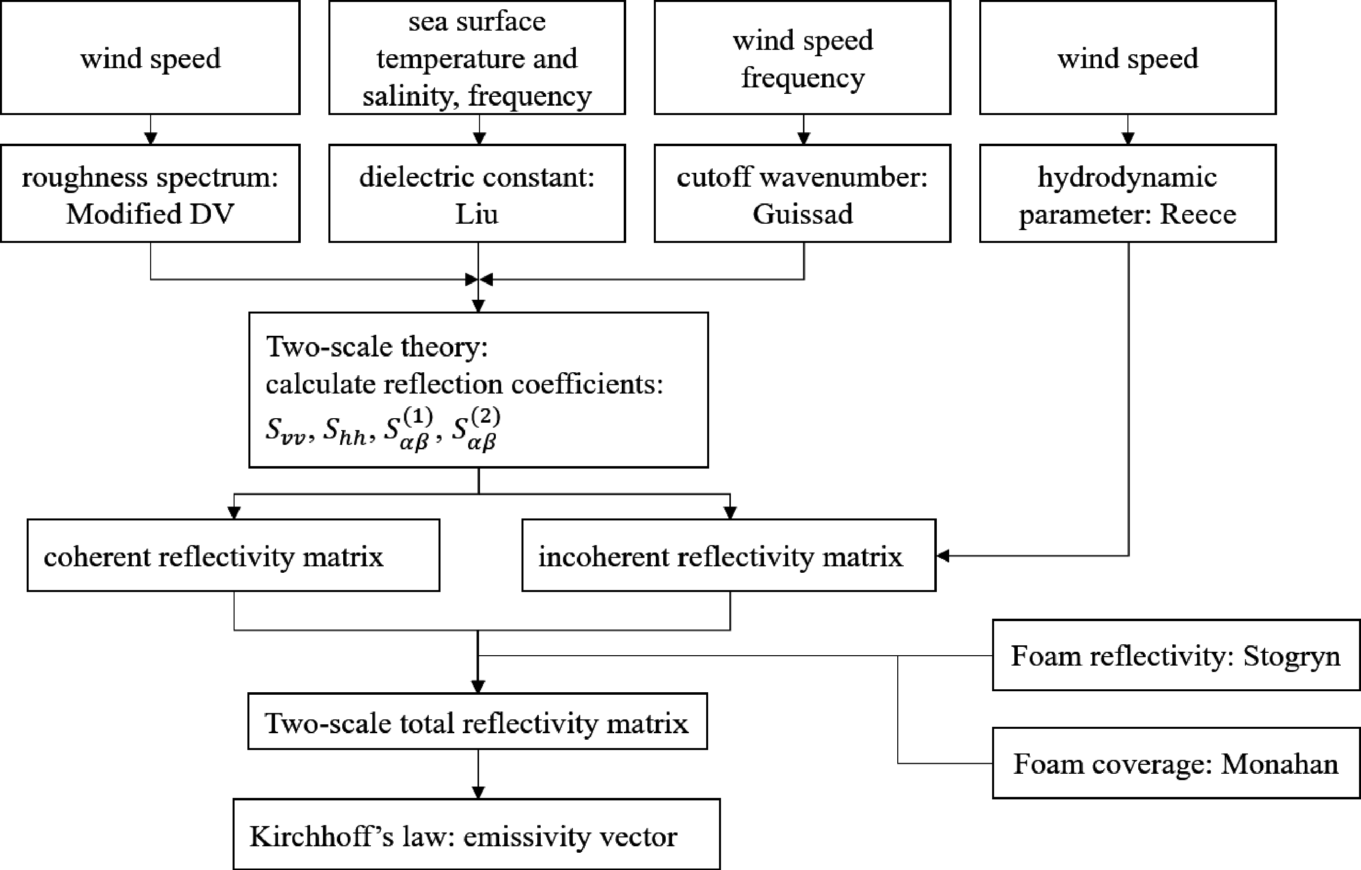
where $ {\mathbf{I}} $ is the Stokes vector; ${\text{ε}}$ is the emissivity vector; ${B_t}$ is the Planck radiance; $ {\mathbf{A}} $ is the reflectivity matrix; $ \mu $ is the cosine of the zenith angle $ \theta $; $ \varphi $ is the azimuth angle. The first term on the right-hand side is the contribution of the emission to the upwelling radiance, and the second term represents the contribution by reflection. Compared with Eq. (12) in the Stamnes’ article, there are two main differences. First, Eq. (20) doesn’t include the solar source term. Second, there is no $ \mu ' $ in the integrand of Eq. (20) because $ {\mathbf{A}} $ is the reflectivity matrix instead of the BRDF.

Figure 2 depicts the above derivation process of the reflectivity matrix and emissivity vector.

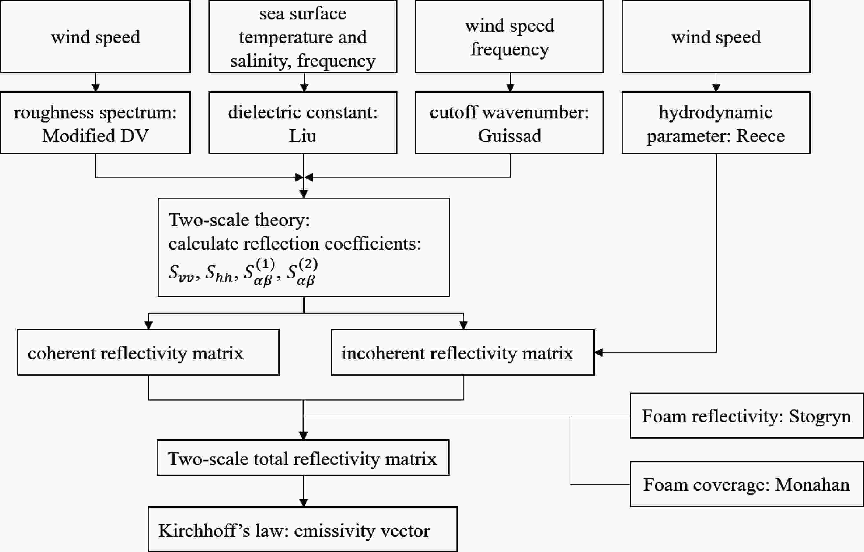
Figure 2.  Flow chart of two-scale reflectivity matrix and emissivity vector models.

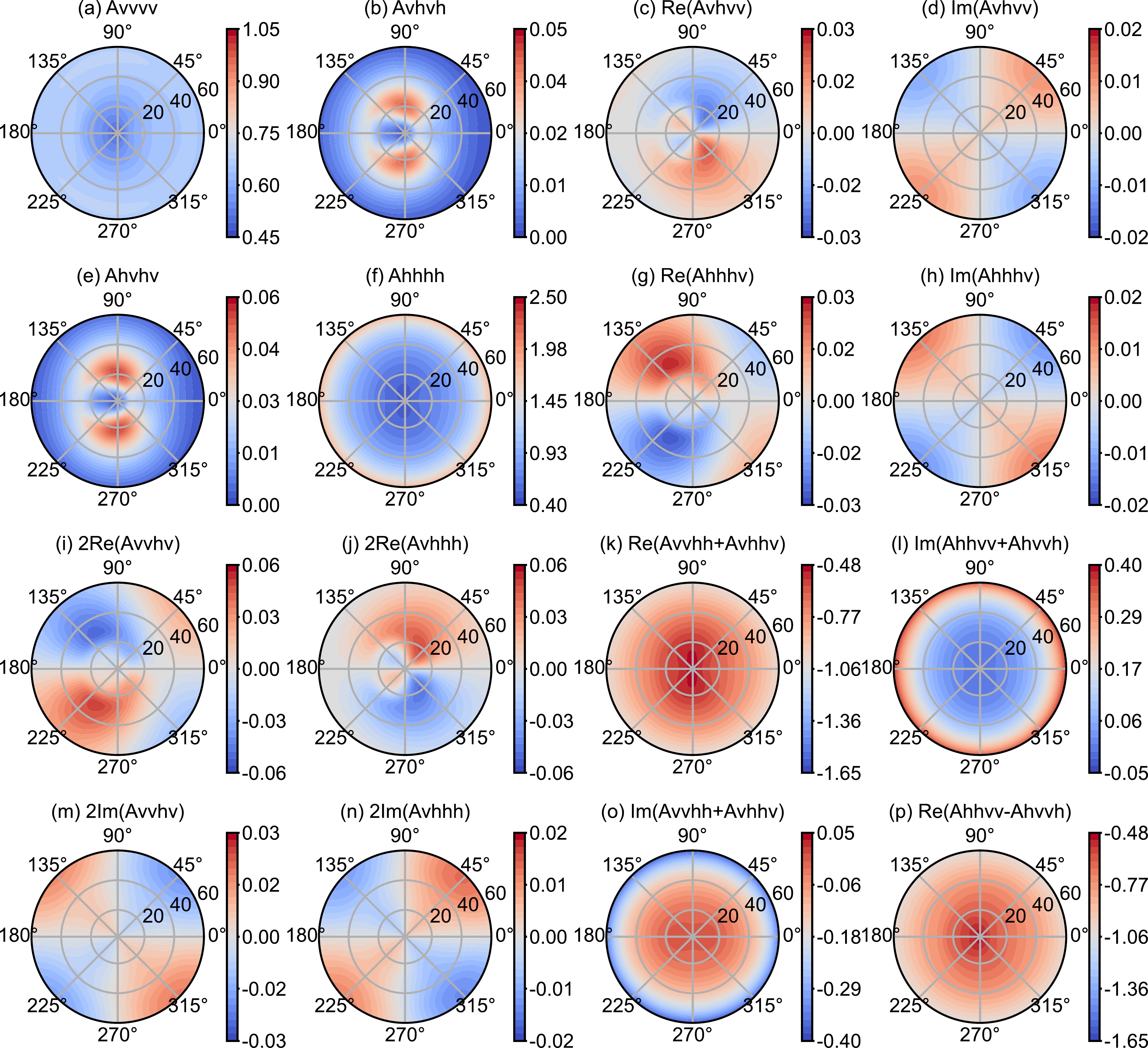
Figures 3–5 depict the distributions of the TSRM in the upper hemisphere in the specular direction $ {\theta _i} = {\theta _s},{\text{ }}{\varphi _i} = {\varphi _s} $ for three microwave frequencies. The specular direction indicates that the incident zenith angle is equal to the scattering zenith angle, and the incident azimuth angle is equal to the scattering azimuth angle. It should be emphasized that the reflectivity matrix relates the incident irradiance and scattered radiance from a small solid angle, so the unit of each matrix element is sr^–1. The value of the reflectivity matrix does not have to be less than one but must be less than one after integrating over the entire upper hemisphere. From Fig. 3, we can easily find that the reflectivity distribution in the upper hemisphere of each element is symmetric with respect to the wind direction. A 0° and 180° azimuth represents the upwind and downwind directions, respectively. According to this symmetrical characteristic, the TSRM can be divided into four 2 × 2 submatrices. The submatrices in the upper-left and lower-right corners are evenly symmetric with respect to the wind direction, and the submatrices in the upper-right and lower-left corners are oddly symmetric.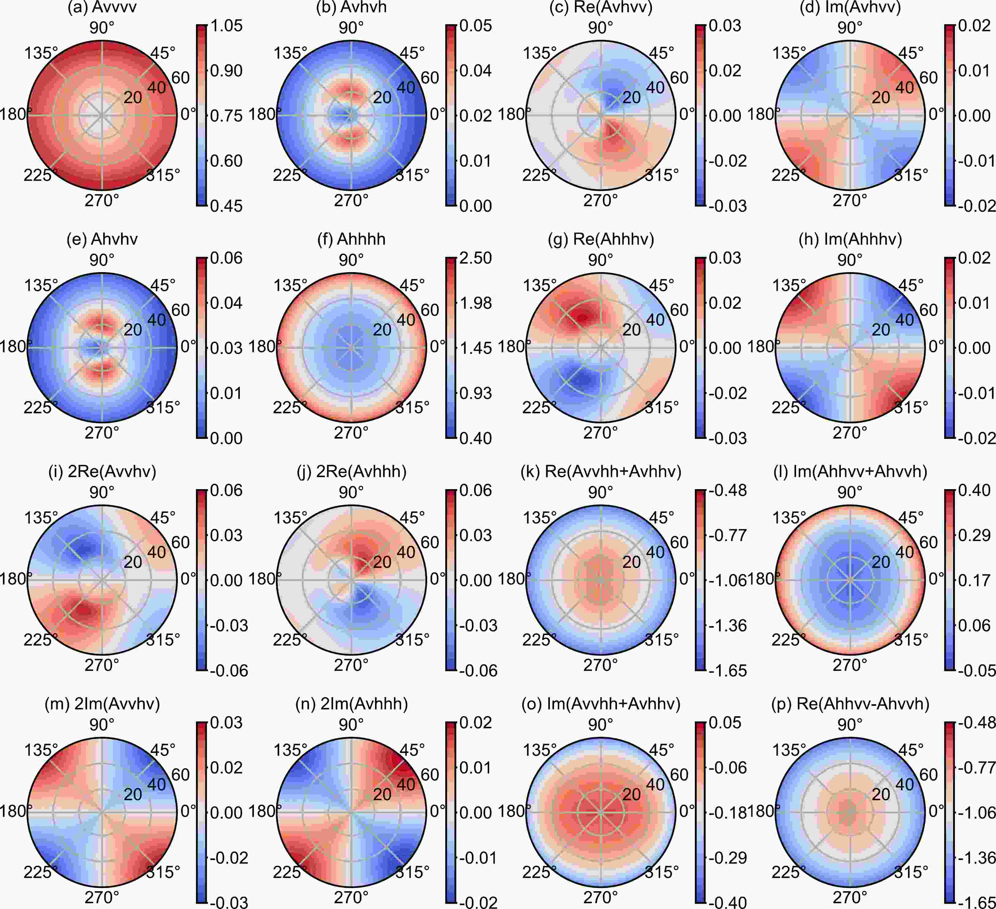

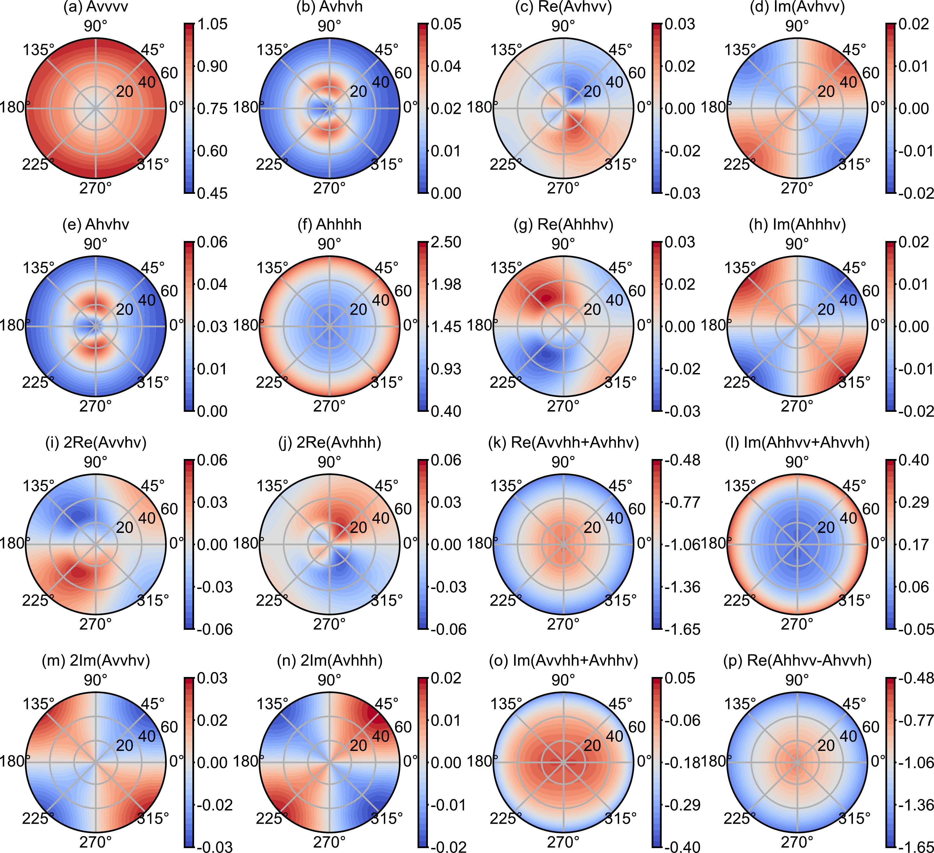
Figure 3.  The TSRM space distribution of 19 GHz at 10 m s^–1 wind speed in the specular direction $ {\theta _i} = {\theta _s},\;{\varphi _i} = {\varphi _s} $. The unit of each matrix element is sr^–1. The sea surface temperature is 285 K, and the salinity is 35‰.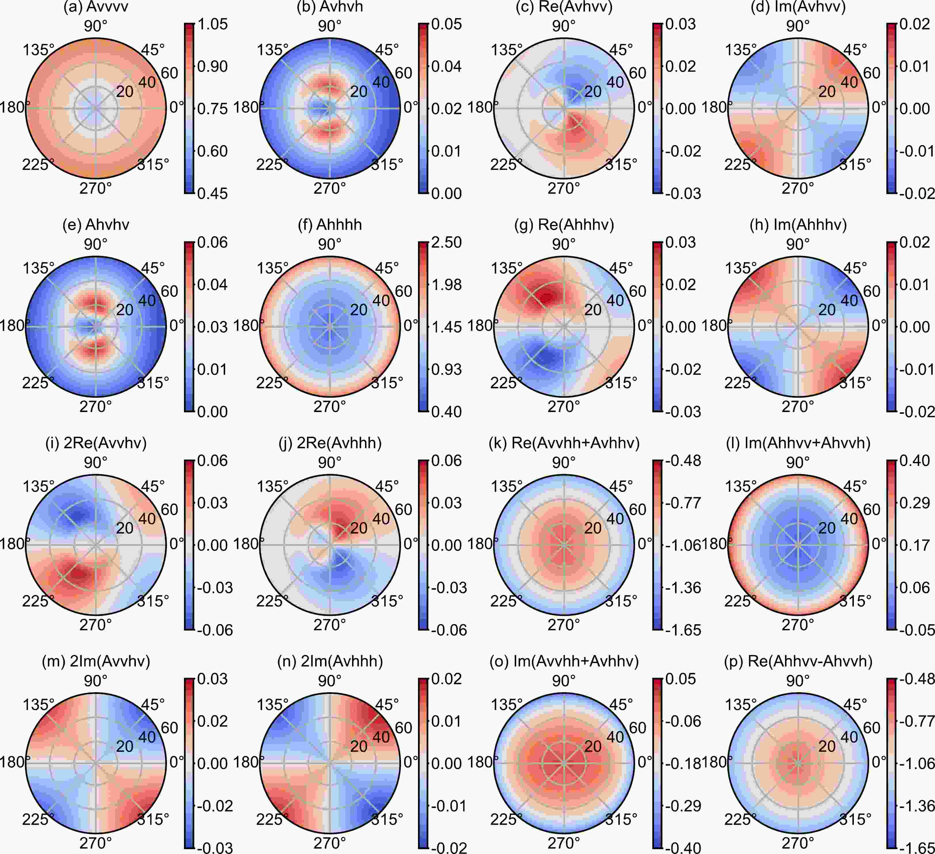

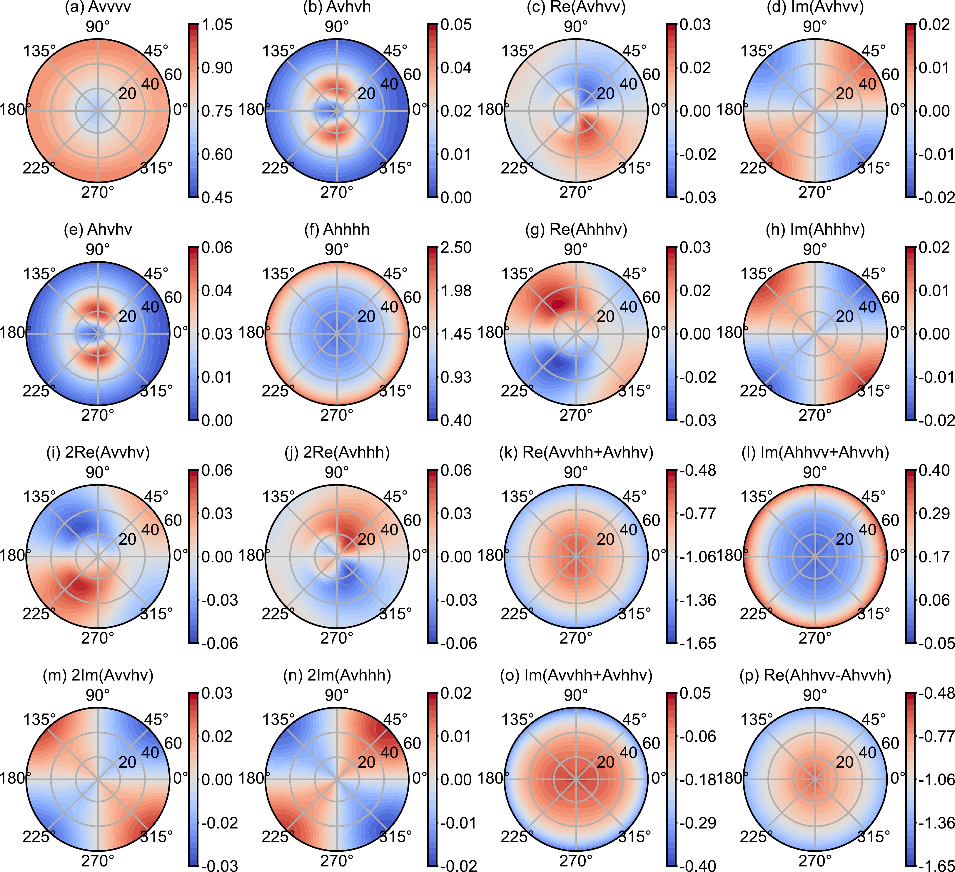
Figure 4.  The TSRM spatial distribution of 23 GHz at 10 m s^–1 wind speed in the specular direction $ {\theta _i} = {\theta _s},{\text{ }}{\varphi _i} = {\varphi _s} $. The unit of each matrix element is sr^–1. The sea surface temperature is 285 K, and the salinity is 35‰.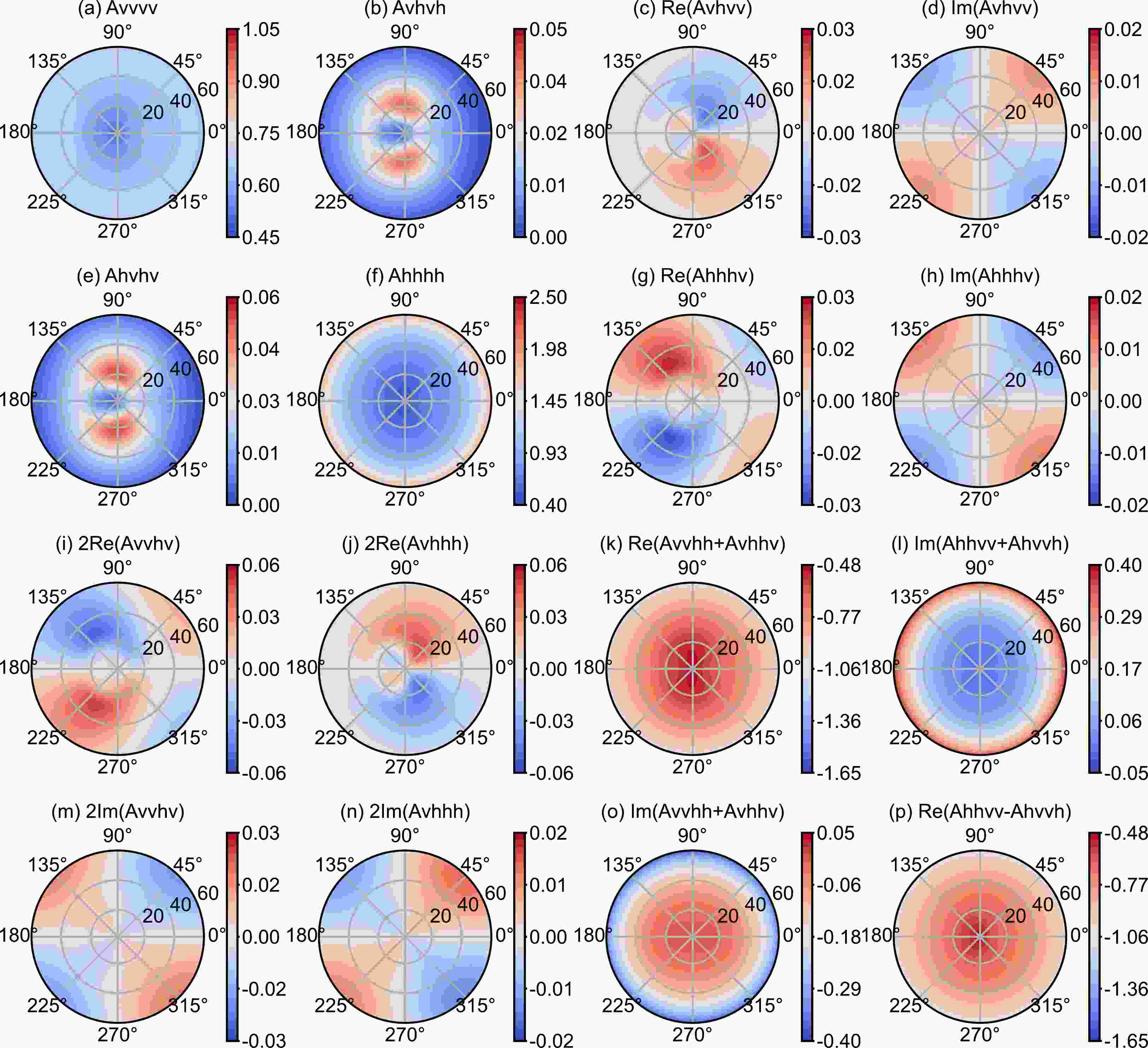

Figure 5.  The TSRM spatial distribution of 37 GHz at 10 m s^–1 wind speed in the specular direction $ {\theta _i} = {\theta _s},{\text{ }}{\varphi _i} = {\varphi _s} $. The unit of each matrix element is sr^–1. The sea surface temperature is 285 K, and the salinity is 35‰

At a certain zenith angles, the TSRM elements exhibit the sine or cosine Fourier harmonic in azimuthal variation. When the zenith angle varies, the azimuthal phases and magnitudes will also change. For a given azimuth angle, each element shows different changes with the increase of the zenith angle. Two elements in the reflectivity matrix with the largest magnitudes were $ {A_{vvvv}} $ (Fig. 3a) and $ {A_{hhhh}} $ (Figs. 3a and 3f, respectively) . Except for $ {A_{vhvh}} $ and $ {A_{hvhv}} $, evenly symmetric elements vary monotonically with zenith angle. The maximum values of both $ {A_{vhvh}} $ and $ {A_{hvhv}} $ occur at the (20º, 90º) and (20º, 270º) positions. The oddly symmetric elements have more significant azimuthal variations than the evenly symmetric elements. All oddly symmetric elements can be divided into two types according to the azimuth position at which the maximum and minimum values occur. In one type are elements ${{\rm{Re}}} ({A_{vhvv}})$ (Fig. 3c), ${{\rm{Re}}} ({A_{hhhv}})$ (Fig. 3g), $2{{\rm{Re}}} ({A_{vvhv}})$ (Fig. 3i), and $2{{\rm{Re}}} ({A_{vhhh}})$ (Fig. 3j). In the other type are the elements $ {{\rm{Im}}} ({A_{vhvv}}) $ (Fig. 3d), $ {{\rm{Im}}} ({A_{hhhv}}) $ (Fig. 3h), $ 2{{\rm{Im}}} ({A_{vvhv}}) $ (Fig. 3m) and $ 2{{\rm{Im}}} ({A_{vhhh}}) $ (Fig. 3n).

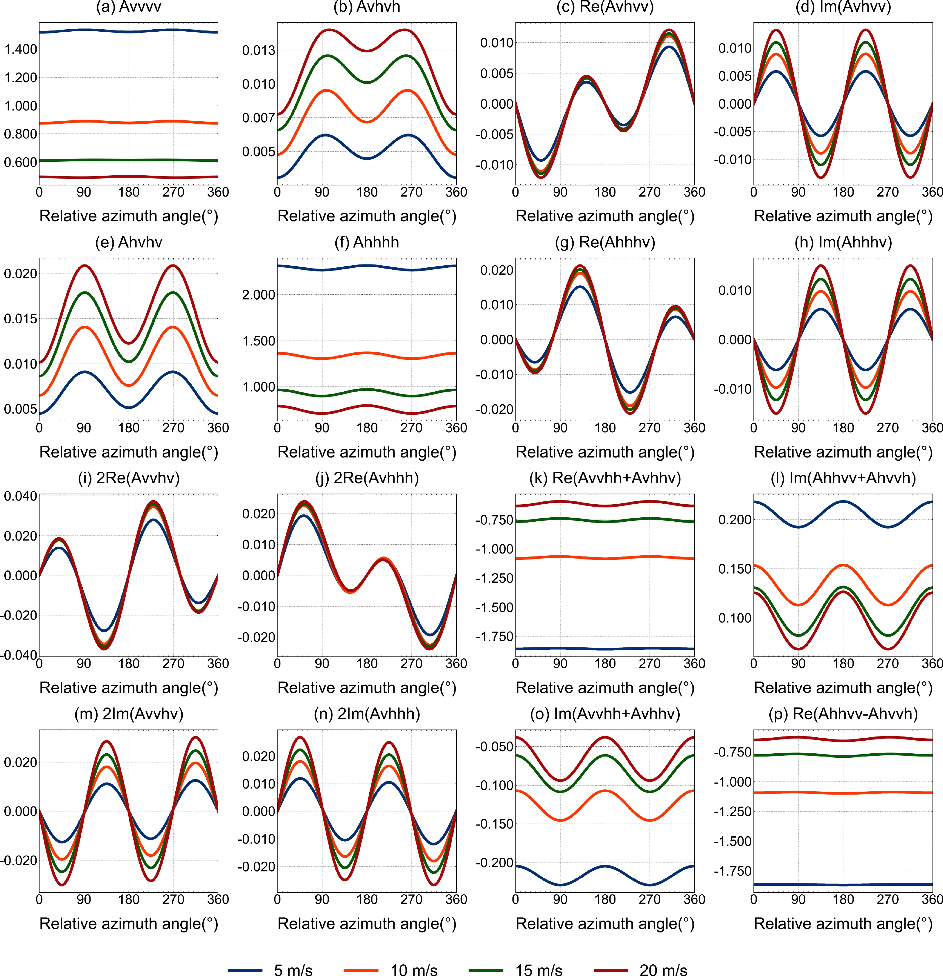
Comparing the results at different frequencies, including 1.58 GHz (not shown), 19 GHz (Fig. 3), 23 GHz (Fig. 4), 37 GHz (Fig. 5), and 89 GHz (not shown), we can find that the reflectivity distribution patterns in the upper hemisphere and values of each element are frequency dependent. In the upper-left submatrices, $ {A_{vvvv}} $ and $ {A_{hhhh}} $ decrease as frequency increases, and the contours gradually change from approximately spherical to elliptical. The long axis of the ellipse points in the direction of the crosswind, which indicates that the difference between the wind direction and the cross-wind direction has increased. As the frequency increases, $ {A_{vhvh}} $ and $ {A_{hvhv}} $ begin to appear as two maxima in the cross-wind direction from 19 GHz. In comparing the evenly symmetric submatrices, we find that the centers of the extremum areas begin to move toward the downwind direction as frequency increases. This indicates that the frequency also affects the symmetry between the upwind and downwind directions. From the variation of elements in oddly symmetric submatrices, we know that the extremum areas move due to the frequency change.

Figure 6 shows the azimuthal variations in the specular direction for the TSRM elements at 23 GHz under different wind speeds. As the wind speed increases, the amplitudes of each element increase, suggesting that an increase in wind speed increases the azimuthal difference; however, the elements do not all increase with wind speed. In fact, values of $ {A_{vvvv}} $ (Fig. 6a) and $ {A_{hhhh}} $ (Fig. 6b) decrease with increasing wind speed because higher wind speeds weaken the reflection in the specular direction and enhances the scattering in other directions. As the wind speed increases, the amplitudes in the azimuth of all oddly symmetric elements increase. The effect of wind speed on the reflectivity matrix elements is dominated by the scattering mechanism. If GO is dominant, the reflectivity element decreases with increasing wind speed. If Bragg scattering is dominant, the reflectivity element increases with increasing wind speed. For example, except for $ {A_{vhvh}} $ (Fig. 6b) and $ {A_{hvhv}} $ (Fig. 6e), which are dominated by Bragg scattering, the other evenly symmetric elements are dominated by GO, so their absolute values all decreased with increasing wind speed. Another notable phenomenon is that the wind speed sensitivity of reflectivity decreases from 20 m s^–1. In general, wind speed has a greater effect on the values of the reflectivity matrix elements than the hemispheric distribution of reflection.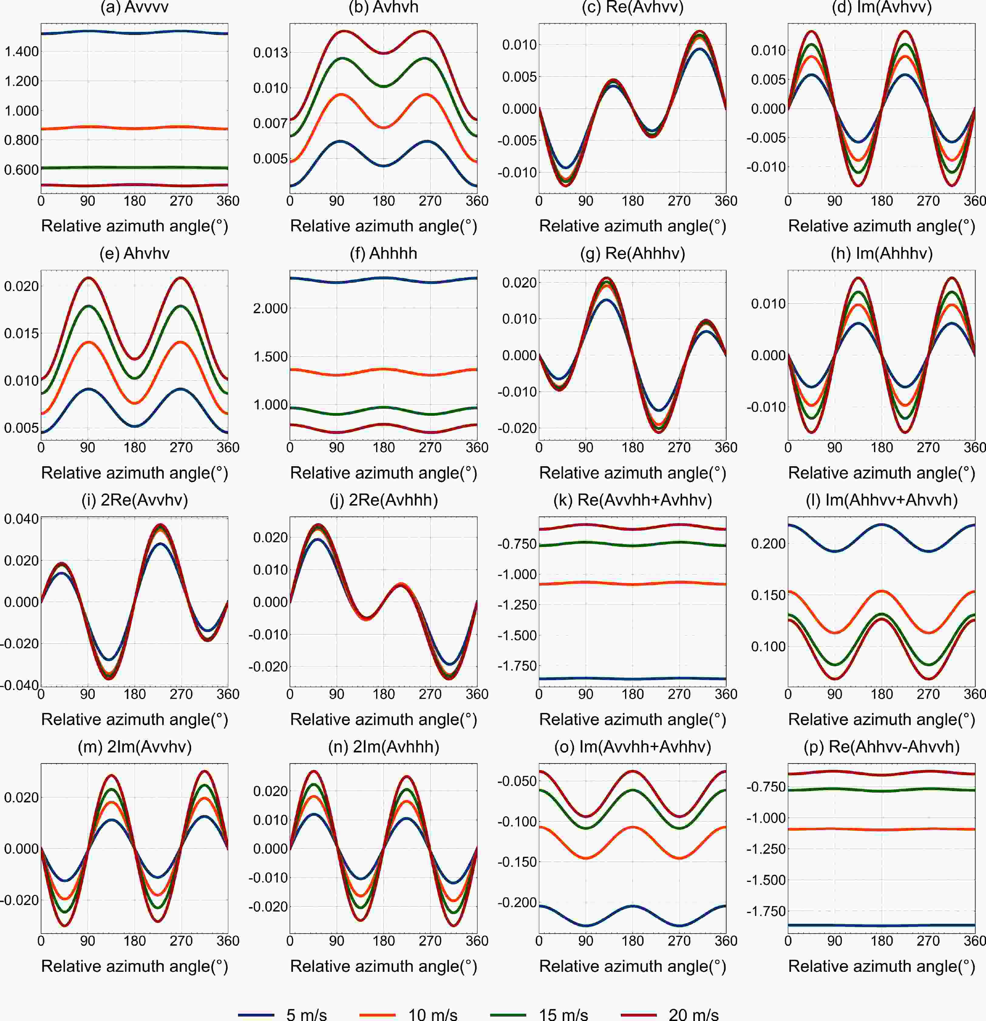

Figure 6.  The TSRM under wind speeds of 5, 10, 15, and 20 m s^–1 as a function of the relative azimuth angle in the specular direction $ {\theta _i} = {\theta _s},\;{\varphi _i} = {\varphi _s} $. The unit of each matrix element is sr^–1. The ocean surface temperature is 285 K, the frequency is 23 GHz, the scattering angle is 45º, and the salinity is 35‰.

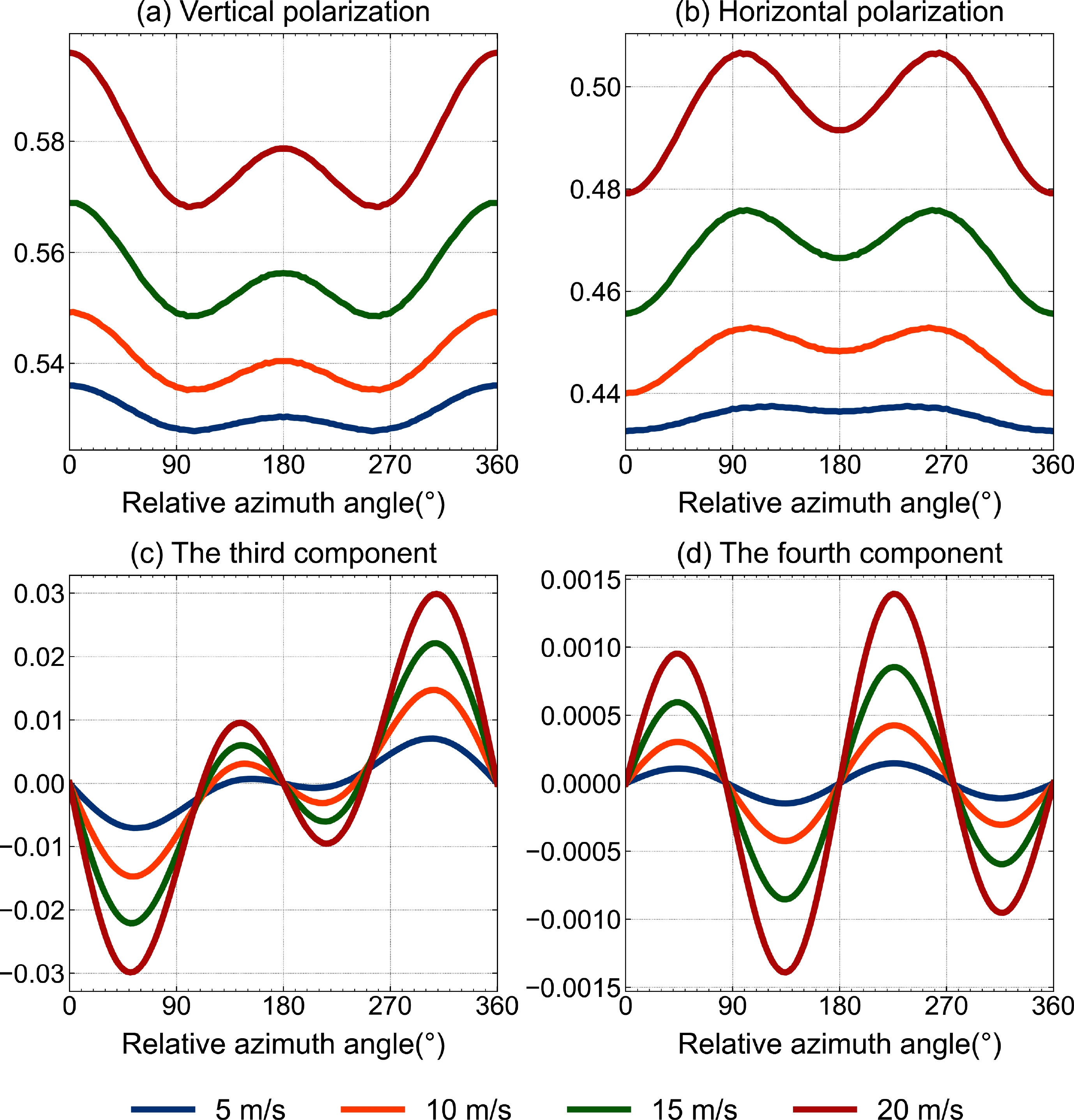
Figure 7 illustrates the TSEM dependence on the relative azimuth angle under the observation zenith angle of 30° for different wind speeds. The azimuthal variations of the vertically (Fig. 7a) and horizontally (Fig. 7b) polarized components in emissivity increase with increasing wind speed and are evenly symmetric with respect to wind direction. For the vertically polarized component, the emissivity in the upwind direction is greater than in the downwind direction, while the opposite is true for the horizontally polarized component. The azimuthal variations of the third (Fig. 7c) and fourth (Fig. 7d) modified Stokes components are oddly symmetric with respect to wind direction, and the oscillation amplitudes increase with wind speed.

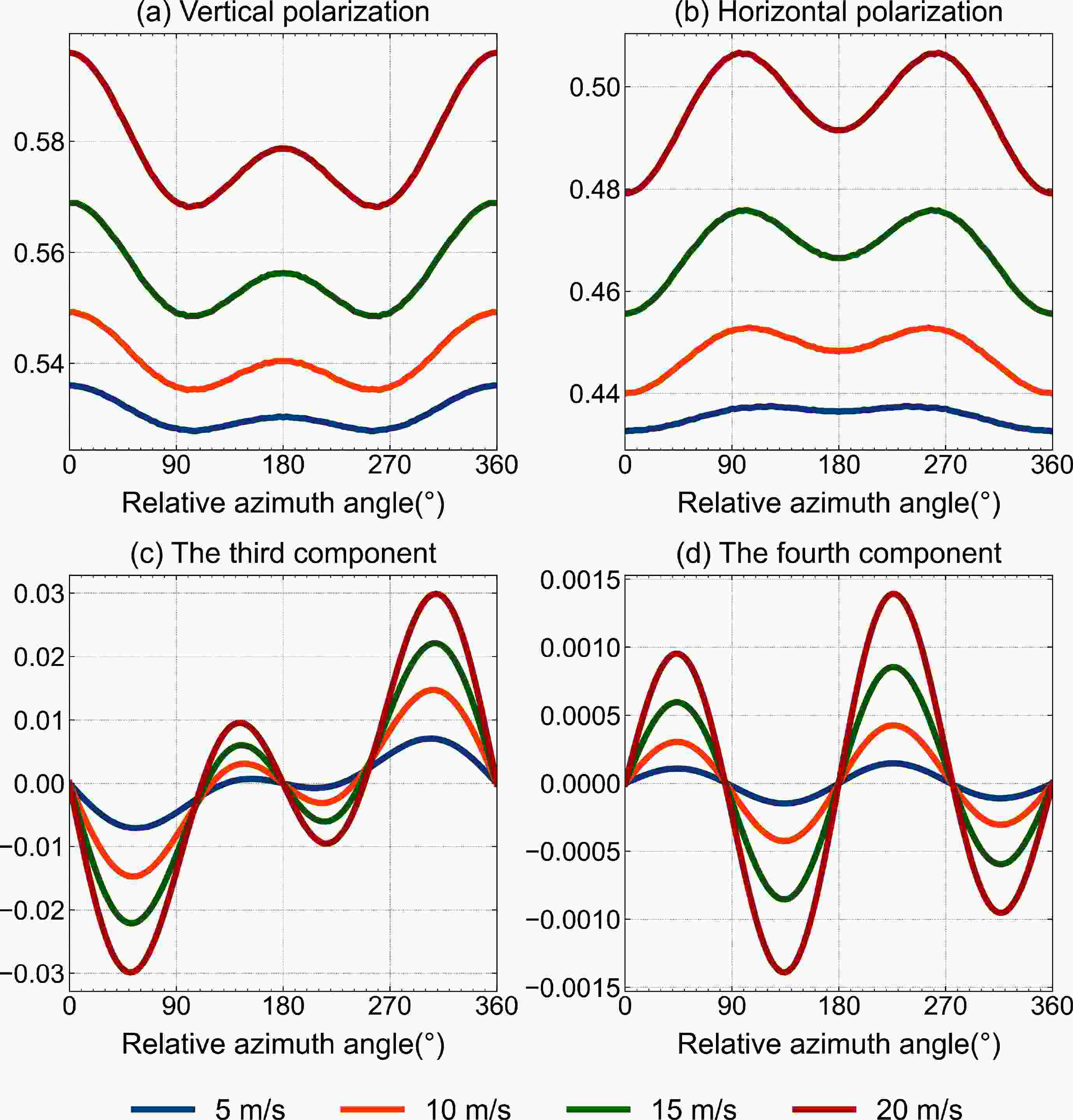
Figure 7.  The TSEM for the (a) vertical polarization component, (b) horizontal polarization component, (c) third component, and (d) fourth component. The TSEM components are calculated as a function of wind speed (5, 10, 15, and 20 m s^–1) and relative azimuth angle. The sea surface temperature is 285 K, the frequency is 37 GHz, the observation angle is 30°, and the salinity is 35‰.

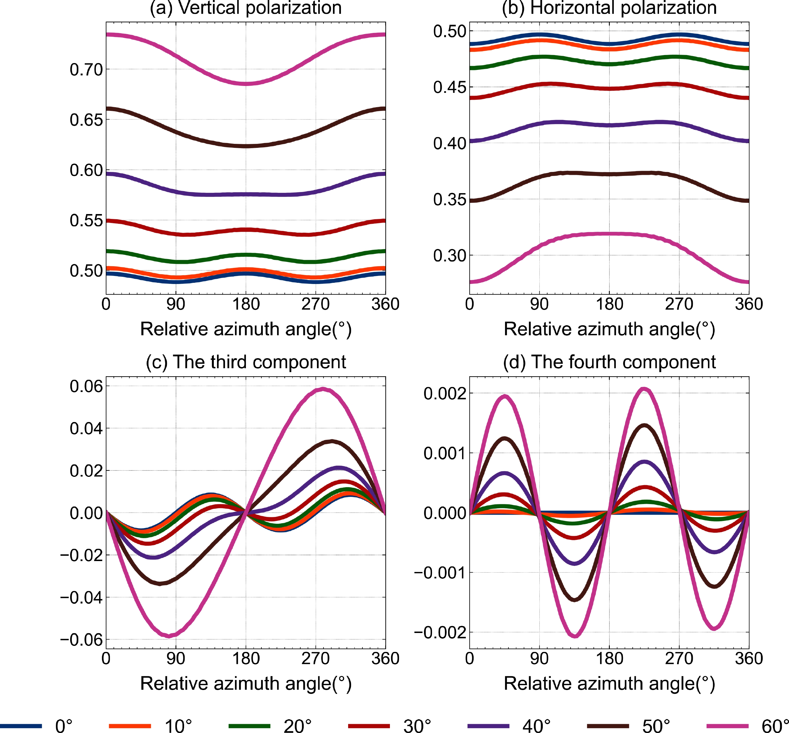
Figure 8 shows the TSEM as a function of the satellite zenith angle and the relative azimuth angle. In the vertical polarization component, the emissivity (Fig. 8a) increases with increasing satellite zenith angle. The peak in the downwind direction fades away, and the $ \cos 2\varphi $ signal gradually becomes a $ \cos \varphi $ signal. For the horizontal polarization component, the emissivity (Fig. 8b) decreases with increasing satellite zenith angle. The dip gradually turns into a peak. The signal of the third component (Fig. 8c) converts from $ \sin 2\varphi $ to $ \sin \varphi $, but the fourth component (Fig. 8d) does not. The oscillation amplitudes of the third and fourth components both increase with increasing satellite zenith angle.

Figure 8.  The TSEM for the (a) vertical polarization component, (b) horizontal polarization component, (c) third component, and (d) fourth component. The TSEM components are calculated as a function of the satellite zenith angle (0°–60°) and the relative azimuth angle. The sea surface temperature is 285 K, the frequency is 37 GHz, the wind speed is 10 m s^–1, and the salinity is 35‰.

The ocean surface is often treated as a collection of wave facets whose reflection is computed through the GO model. According to the Fresnel equations, the reflectivity matrix $ {{\mathbf{A}}_{GO}} $ for the ocean facets is expressed as follows:

where $ {S_{vv}} $ and $ {S_{hh}} $ are the vertical and horizontal polarization Fresnel reflection coefficients, respectively. $ S_{vv}^* $ and $ S_{hh}^* $ are their corresponding complex conjugate. $ {{\mathbf{R}}_{GO}} $ is the GO reflection coefficients matrix. The other parameters, except for $ {{\mathbf{R}}_{GO}} $ in Eq. (22), are defined in the same way as in Eq. (9). Comparing Eqs. (23) and (13), we see that most of the elements in the reflection matrix are zero in the GO model. Also, the GO model cannot predict the cross-polarization elements, $ {A_{vhvh}} $ and $ {A_{hvhv}} $, from the facet tilting and the second-order Bragg scattering. Here, we compare the reflected radiation calculated from the GO reflectivity matrix and the TSRM, respectively. First, the atmospheric downwelling radiances are calculated from MonoRTM, and the reflected radiation, the second term in Eq. (20), is then calculated using two different reflectivity matrices. MonoRTM is a radiative transfer model designed to calculate the radiances at monochromatic wavelengths and is widely used in microwave spectral regions (Clough et al., 2005). A U.S. standard atmospheric profile is used as input, and ocean surface wind speed, sea surface temperature, and seawater salinity are assumed to be 10 m s^–1, 285 K, and 35‰, respectively.

Figure 9 shows the difference between radiation reflected by the GO reflectivity matrix model and the TSRM at 23.8 GHz. The TSRM consists of three parts, the large-scale GO contribution, the small-scale contribution of the first-order incoherent scattering term SPM1, and the second-order coherent reflection term SPM2. We can see that the effects of the small scale on the reflected BT Stokes components are different. The small scale reduces the horizontal (Fig. 9b) and vertical (Fig. 9a) components while it increases the third (Fig. 9c) and fourth (Fig. 9d) components. However, the effects of SPM1 and SPM2 are different. SPM2 enhances the difference between the GO model and TSRM, while SPM1 reduces this difference. It can be seen that the GO model cannot contribute to the third and fourth components. The third and fourth components have BT differences of 0.5–1.5 K and 0.2 K with the increasing satellite zenith angle, respectively. Overall, the smallest vertical and horizontal differences both occur at about a 20° satellite zenith angle, while the largest difference is about 5 K in the horizontal component at 23.8 GHz at large satellite zenith angles. The differences among the four Stokes components as a function of satellite zenith angle have obvious frequency dependences (not shown). It must be noted that the differences also change with the relative azimuth angle.

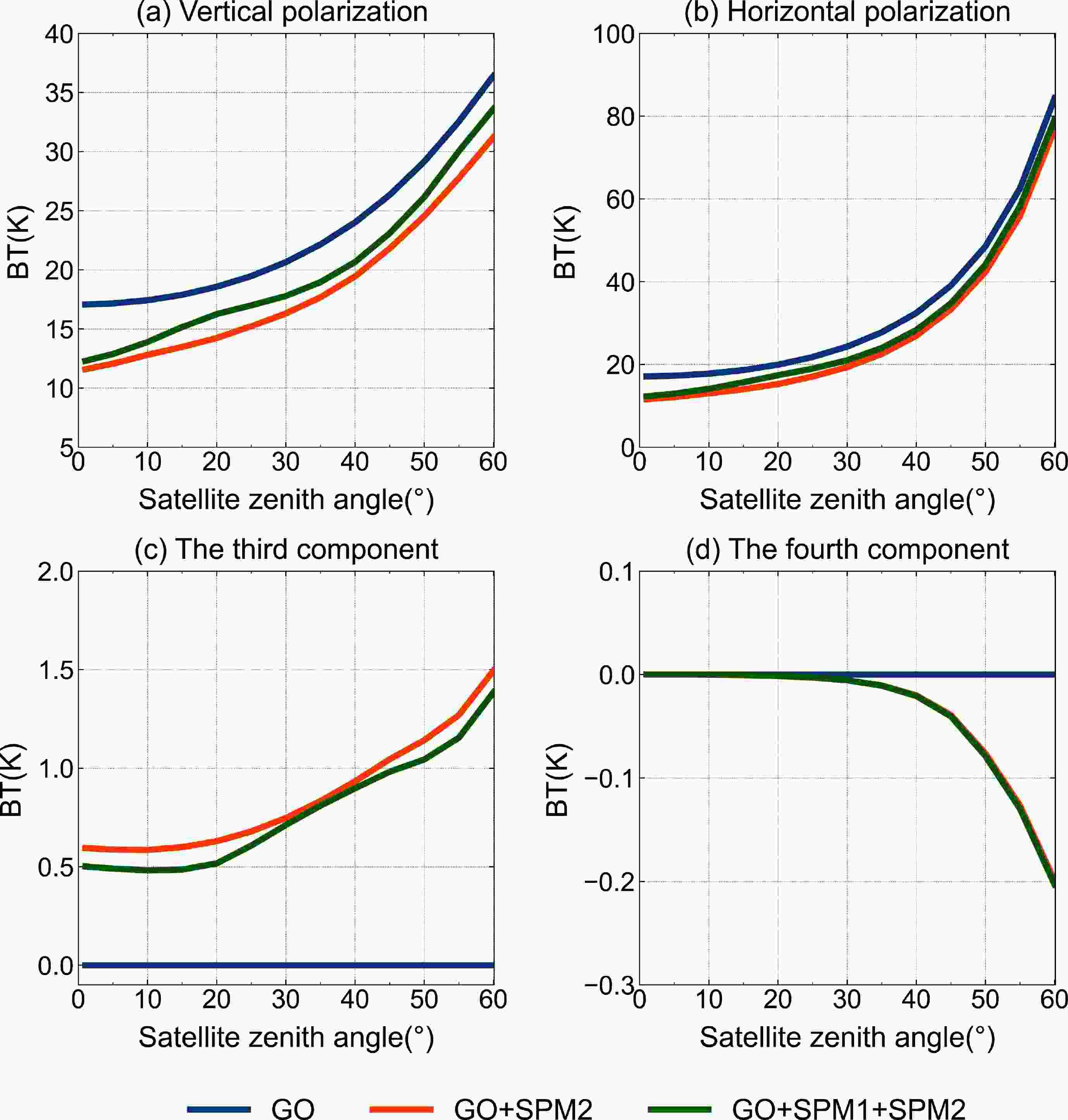
Figure 9.  The reflected BT Stokes vector for the (a) vertical polarization component, (b) horizontal polarization component, (c) third component, and (d) fourth component. They are calculated as a function of the satellite zenith angle (0°–60°). The sea surface temperature is 285 K, the frequency is 23.8 GHz, the wind speed is 10 m s^–1, and the salinity is 35‰. The relative azimuth angle is 45°.

Previously, the model FASTEM was developed for computationally fast and accurate ocean surface emissivity results in data assimilation community. FASTEM has undergone several updates from version 1 to 6. FASTEM1 and 2 were both based on GO model simulation results, but version 2 is added with an exponential reflectivity correction compared to version 1. FASTEM3 introduced a relative wind direction (RWD) model function for the first time. FASTEM4 updated the permittivity model, foam and roughness effect parameterizations, and the RWD. FASTEM5 reverted to the former foam-cover model, and version 6 was similar to version 5 but had a new RWD. The RWDs of FASTEM4 and 5 were developed based on a theoretical two-scale model output, while version 6 was based on satellite measurements (Kazumori and English, 2015). FASTEM6 has been calibrated and validated operationally and is used for our analysis. Here, we use FASTEM6, hereafter referred to as FASTEM.

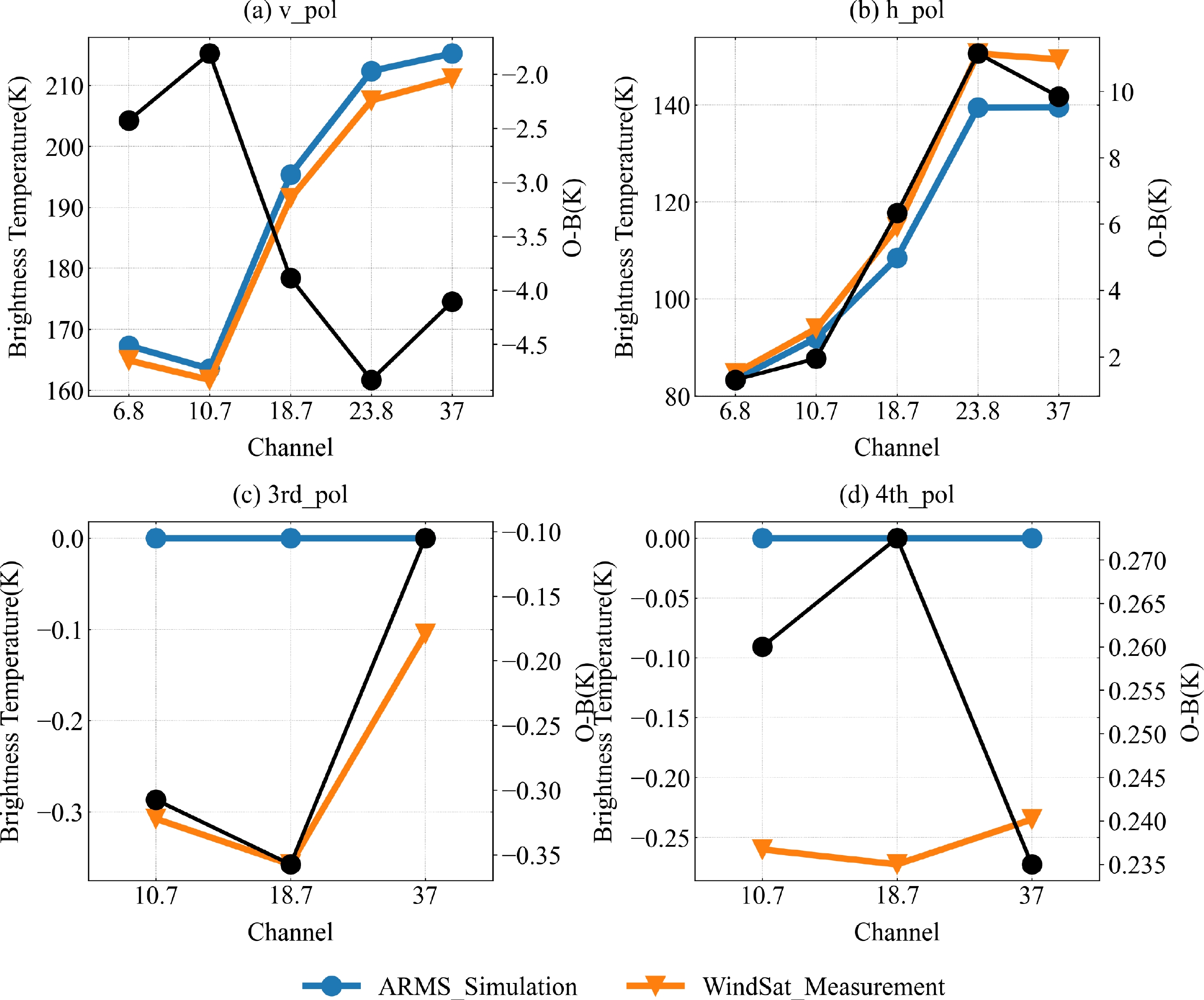
The three main fast radiative transfer models, CRTM, RTTOV, and ARMS, all adopt FASTEM to calculate the ocean emissivity vector and then use non-polarized radiance Stokes vector with unit amplitude minus the emissivity vector to obtain the reflectivity vector, to be corrected by a transmittance factor, which is called FASTEM scheme. Figure 10 shows the difference between the modified Stokes vectors simulated at the top of the atmosphere (TOA) from ARMS and WindSat observations. WindSat is the first space-borne polarimetric microwave radiometer developed by U.S. Navy for measuring ocean surface wind speed and direction. WindSat operates at 6.8, 10.7, 18.7, 23.8, and 37.0 GHz. The 10.7, 18.7, and 37 GHz channels are fully polarimetric, while the 6.8 and 23.8 GHz channels are dual polarimetric. As a polarimetric radiometer, WindSat measures not only the principal polarizations (vertical and horizontal) but also the cross-correlation of the vertical and horizontal polarization. The cross-correlation terms represent the third and fourth parameters of the modified Stokes vector. The simulation results at the lower boundary are based on the FASTEM scheme. From Fig. 10, we can find that the FASTEM scheme bias reaches 4.5 K in vertical polarization, reaches 10 K in horizontal polarization, and cannot predict the third and fourth parameters.

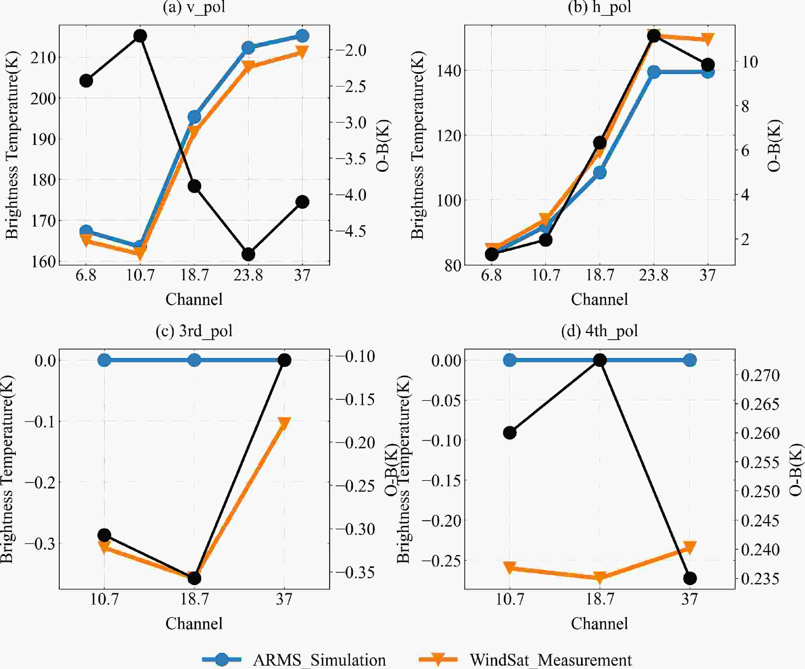
Figure 10.  Simulated TOA brightness temperatures by ARMS and WindSat measurements for the modified Stokes vector. Black lines represent the difference (measurement minus simulation). The wind speed is 10 m s^–1, and the relative azimuth angle is 45°.

Figure 11 shows the difference in emitted radiation between TSEM and FASTEM. The current version of FASTEM does not have the third and fourth Stokes components, so only the vertical and horizontal components are compared here. For the vertical polarization component (Fig. 11a), the difference at each frequency has an extreme value at a large angle which is related to the Brewster angle because both TSRM and TSEM include the coherent reflection. Unlike TSEM, FASTEM has a lack of Brewster angle effect in and results in the extreme value in the difference. The Brewster angle is smaller at higher frequeny. Note that the difference begins to decrease when the satellite zenith angle is greater than the Brewster angle. The largest difference in the vertical component is about 8 K. Overall, the horizontal difference is larger than the vertical component (Fig. 11b). The larger the satellite zenith angle and the higher the frequency, the larger the difference. The largest difference in horizontal difference is about 21 K. The FASTEM was not parameterized to operate at large satellite zenith angles (Prigent et al., 2017); therefore, the calculation of the emitted radiation is problematic because it needs to be calculated in all directions. The emitted BTs calculated from TSEM are less than FASTEM, especially at large satellite zenith angles. Thus the emissivity calculated by FASTEM is too large and is becoming a problematic at large angles.

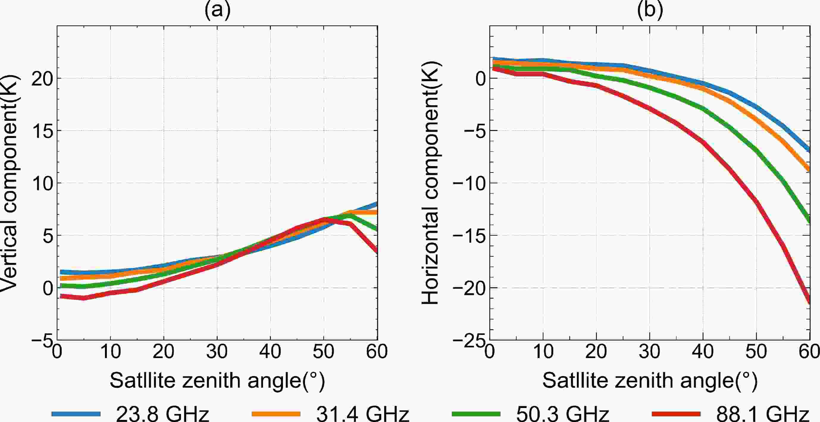
Figure 11.  The difference (TSEM minus FASTEM) of emitted BT for the (a) vertical polarization component and (b) horizontal polarization component. The difference is a function of the satellite zenith angle (0°–60°) under different frequencies at 23.8 GHz, 31.4 GHz, 50.3 GHz, and 88.1 GHz. The sea surface temperature is 285K, the wind speed is 10 m s^–1, and the salinity is 35‰. The relative azimuth angle is 45º.

In this study, a generic ocean microwave reflectivity matrix and emissivity model are developed from two-scale anisotropic roughness theory. In addition to the GO and FASTEM, other studies have used two-scale roughness theory; however, two-scale roughness theory is rarely used to develop the reflectivity matrix, emissivity model, and the backscattering cross-section of the ocean surface consistently. Jin et al. (2021) derived a two-scale reflectivity matrix, but the dielectric model only applied to the L-band. The dielectric constant model and a flexible cutoff wavenumber scheme developed by Liu et al. (2011) make the TSRM applicable for a wider range of microwave frequencies, and the modified DV spectrum makes the TSRM suitable for a wider range of zenith angles and wind speeds. This study also focuses on the characteristics of the elements of the reflectivity matrix and analyzes the dependence of all elements of the TSRM and TSEM on the zenith angle, azimuth angle, frequency, and wind vector. Furthermore, a set of downwelling radiances at different frequencies using MonoRTM are simulated to compare the reflected radiation differences between the TSRM with the GO reflectivity matrix model and the emitted radiation differences between the TSEM with FASTEM.

The 16 elements of the TSRM have obvious symmetry with respect to the wind direction. The dominant scattering mechanism affects the dependence of different TSRM elements on zenith angle, wind speed, and frequency. Compared with the previous GO reflectivity matrix, the TSRM can predict the behaviors of all the elements, including the evenly symmetric $ {A_{vhvh}} $ and $ {A_{hvhv}} $; and the remaining oddly symmetric elements. The TSRM includes three parts: the large-scale part (same as GO), the small-scale incoherent part, and the coherent part. The small-scale effect decreases the vertical and horizontal reflected radiation and increases the third and fourth components reflected radiation. The radiation difference is about 5 K at a frequency of 23.8 GHz, and the differences exhibit a frequency dependence. From the Kirchhoff’s law, the TSEM is derived from the TSRM. This method is different from the traditional two-scale emissivity. The TSEM can reasonably reflect the wind direction information, and its numerical accuracy is comparable to that of FASTEM at small satellite zenith angles, which proves the reliability of the TSEM. The emitted radiation difference between the TSEM and FASTEM is less than 5 K when the satellite zenith angle is less than 40°. The large negative difference at large angles in the horizontal component implies that TSEM is more accurate for large angles than FASTEM.

This study preliminarily proves the feasibility and rationality of the physical TSRM and TSEM required at the lower boundary condition in a radiative transfer scheme. The accuracy of the TSEM and TSRM used for the lower boundary scheme will be further evaluated after they are fully integrated into the vector radiative transfer model. At present, the sea foam reflectivity matrix is simple but exerts an important influence on the distribution of ocean surface radiation, especially in high wind-speed conditions. Also, we have not considered the effect of breaking waves and multiple scattering effects, which are significant at large zenith angles. These aspects will limit the zenith angle range. In our future research, the two-scale reflectivity matrix model will be further improved to address these shortcomings.

Acknowledgements. This study is funded by the National Key Research and Development Program (Grant No. 2022YFC3004200), the National Key Research and Development Program of China (Grant No. 2021YFB3900400), Hunan Provincial Natural Science Foundation of China (Grant No. 2021JC0009), and the National Natural Science Foundation of China (Grant No. U2142212).