


 DownLoad:


-
Spectral variations in atmospheric radiation provide extensive information for remote sensing of atmospheric temperature, gas, aerosol, and cloud properties (Liou, 1992, 2002). Hyperspectral radiometric sounders have become an essential and unique part of atmospheric monitoring from space. Data from hyperspectral infrared (IR) instruments, such as the Atmospheric Infrared Sounder (AIRS) on the Aqua satellite, the Infrared Atmospheric Sounding Interferometer (IASI) on the MetOp satellites, the Cross-Track Infrared Sounder (CrIS) on the Suomi National Polar-orbiting Partnership and Joint Polar Orbit Satellite System series, and the High-spectral Resolution Infrared Atmospheric Sounder (HIRAS) on the Fengyun-3D satellite, have been widely used for nowcasting, numerical weather prediction (NWP), environmental monitoring and climate studies (Li et al., 2018; Menzel et al., 2018). Meanwhile, the Geosynchronous Interferometric Infrared Sounder (GIIRS), the first geostationary hyperspectral IR sounder onboard the Chinese Fengyun-4A (FY-4A) and Fengyun-4B (FY-4B) satellites (Yang et al., 2017), is expected to infer continuous atmospheric vertical temperature and moisture structures for various applications such as high-impact weather situational awareness with atmospheric thermodynamic and dynamic information, data assimilation for improving regional and global NWP, monitoring and understanding diurnal variations of atmospheric parameters, etc. (Crevoisier et al., 2004; Burrows et al., 2021; Schmetz, 2021; Li et al., 2022a).
With IR sounders continually becoming upgraded and operational, corresponding forward hyperspectral radiative transfer models (HRTM) are always essential for their calibration, assimilation, and quantitative applications. Due to the significant spectral variation in atmospheric molecular absorptions, HRTM must be performed at a very fine spectral resolution, which may be at least an order of magnitude higher than the instrument resolution. The line-by-line-based (LBL) radiative transfer approach is a standard approach for accurate HRTM simulations, while the large number of monochromatic simulations required by quantitative applications makes LBL models impractical in terms of computational resources (Zhang et al., 2005).
Thus, several fast HRTMs have been developed (Duan et al., 2010; Natraj et al., 2005; Liu et al., 2006; Moncet et al., 2008; Wang et al., 2013; Efremenko et al., 2014; Wang et al., 2015; Li et al., 2017; Li et al., 2018). Statistical methods, such as the optical path transmittance model (McMillin et al., 1995), use the statistical relationships between channel transmittances and predictors (e.g., atmospheric profiles and observation geometry), so the atmospheric transmittance can be calculated efficiently. However, the choice of the predictors is empirical, and its accuracy becomes limited in a complex absorption band. The Optimal Spectral Sampling (OSS) used for producing the operational CrIS products is based on a weighted average of well-trained monochromatic radiances at selected nodes and is more accurate for complex absorption bands (Moncet et al., 2008). Bai et al. (2016) further improved OSS by maximizing the use of duplicate channels and eliminating duplicate information nodes to achieve higher computational efficiency. The correlated k-distribution method (Shi, 1998; Zhang and Shi, 2000) also leads to larger errors for inhomogeneous atmospheres or optical paths. Thus, there are also many derivative methods based on it, such as the full-spectrum correlation k-distribution (FSCK) method (Wang et al., 2019) which is based on pre-generated look-up tables (LUTs). Those models select enough samples and contain a wide range of atmospheric contours in the LBL model to obtain the exact monochromatic atmospheric transmittance. However, the LUT size may be quite significant for practical applications (Wang et al., 2019). Meanwhile, a weighted least squares method is used for the Radiative Transfer for Television and Infrared Observation Satellite (TIROS) Operational Vertical Sounder (RTTOV), which is developed by the numerical weather prediction (NWP) Satellite Application Facility from EUMETSAT (EUropean Organisation for Exploitation of METeorological SATellites) (Li et al., 2000; Matricardi, 2008; Zhang et al., 2014, 2016), and Di et al. (2018) further enhanced its accuracy for GIIRS simulations by using local training atmospheric profiles. Similarly, the Community Radiative Transfer Model (CRTM) uses several statistical regression methods (optical depth in pressure space and absorber space) for the gas transmittances (McMillin et al., 1995; Han et al., 2006; Chen et al., 2008; Karpowicz et al., 2022). These models have played important roles in hyperspectral measurement applications, while the requirements for the efficiency and accuracy of RT models are always increasing.
Principal component analysis (PCA) is a general numerical method to reduce the dimensionality of a problem based on the linear relationship among the variables (Antonelli et al., 2004), and the PCA-based HRTMs have been well developed and improved (Liu et al., 2006, 2016). By extending a very small fraction of radiances to those of the full spectrum using the PCA method, models of this kind can significantly reduce the number of monochromatic simulations in the HRTM and are found to be reliable for both clear and cloudy atmospheres. The PCA-based models have been well used for AIRS and NAST-I instruments (Liu et al., 2006) as well as the RTTOV model (Matricardi, 2010). Meanwhile, Natraj et al. (2005) developed a PCA-based model in the aerosol optical domain to accelerate monochromatic simulations, and Liu et al. (2020) combined the two kinds of PCA-based models to optimize HRTM computational efficiency.
In recent years, machine learning (ML) techniques have become a powerful and popular method for big data processing (Jordan and Mitchell, 2015; Poostchi et al., 2018) and are also tested for RT simulations by developing complex relationships between atmospheric parameters and radiative variables (Dorvlo et al., 2002; Takenaka et al., 2011). As one of the first applications, Chevallier et al. (1998) used NN in longwave RT. The ML-based FSCK uses a biological neural network to reduce LUT storage (Zhou et al., 2020). Le et al. (2020) introduced a model based on the neural network (NN) to extend a small fraction of monochromatic radiances to the entire spectral range, which can capture the non-linear relationships among the spectral radiances. Stegmann et al. (2022) have also used an NN for fast transmittance parameterization in radiative transfer models and show great potential for operational remote sensing and data assimilation applications. In addition, a recurrent NN (RNN) method was developed to structurally incorporate the vertical dependence and sequential nature of radiation computations (Ukkonen, 2022), which can predict fluxes with relative differences of less than 1% and heating rates with root mean square error (RMSE) less than 0.16 K d–1. With ML techniques applied in more and more RT simulations in different ways (e.g., Le et al., 2020; Liang and Liu, 2020; Stegmann et al., 2022), traditional (e.g., the aforementioned PCA-based models) and ML-based models were also briefly compared, noting that further studies are still needed to better understand their capabilities and advantages/disadvantages.
To summarize, most of the aforementioned PCA or NN-based HRTMs focus on the reduction of the number of independent RT simulations needed (Liu et al., 2006) or on treatments related to scattering simulations (Natraj et al., 2005; Wang et al., 2015), while monochromatic gas absorption or transmittance simulations are less discussed, which are also time-consuming. Actually, PCA and NN can make similar calculations for extending a small amount of data to a large amount of the same kinds, i.e., in the sense of data compression/extension, while the former accounts for their linear relationships and the latter obtains complex non-linear relationships. Therefore, this study intends to introduce the multi-domain PCA/NN method to further improve HRTM efficiencies and systematically evaluate PCA- and NN-based models. Because we use either the PCA or NN method independently to compress the information in HRTM to reduce the computational burden in both gas transmittance and radiance domains, the new method will be referred to as a multi-domain compression method. Furthermore, the model is particularly designed for the GIIRS bands to serve its scientific and operational applications.
The remainder of this paper is organized as follows. Section 2 introduces our multi-domain compression method. Section 3 details the preparations for the pre-calculated and pre-trained datasets used for the methods, in addition to comparing model performances and comparisons. Section 4 provides a summary and conclusion for this study.
-
One of the key tasks for high-spectral radiative transfer simulations is that calculations of the same kind must be carried out multiple times in both the atmospheric (different atmospheric conditions) and spectral (different wavenumbers) domains. For example, gas transmittances at each wavenumber for each layer are needed, and RT simulations are performed for each monochromatic wavenumber, which should have a spectral resolution much finer than the instrument resolutions. Thus, the essence of our model is to reduce those independent simulations in the RT simulations as much as possible. In other words, we try to perform only a small fraction of those repeated simulations and extend them to the complete information needed. The extension, which can be done differently, should be much less time-consuming, and this study performs the extension based on the PCA and ML methods.
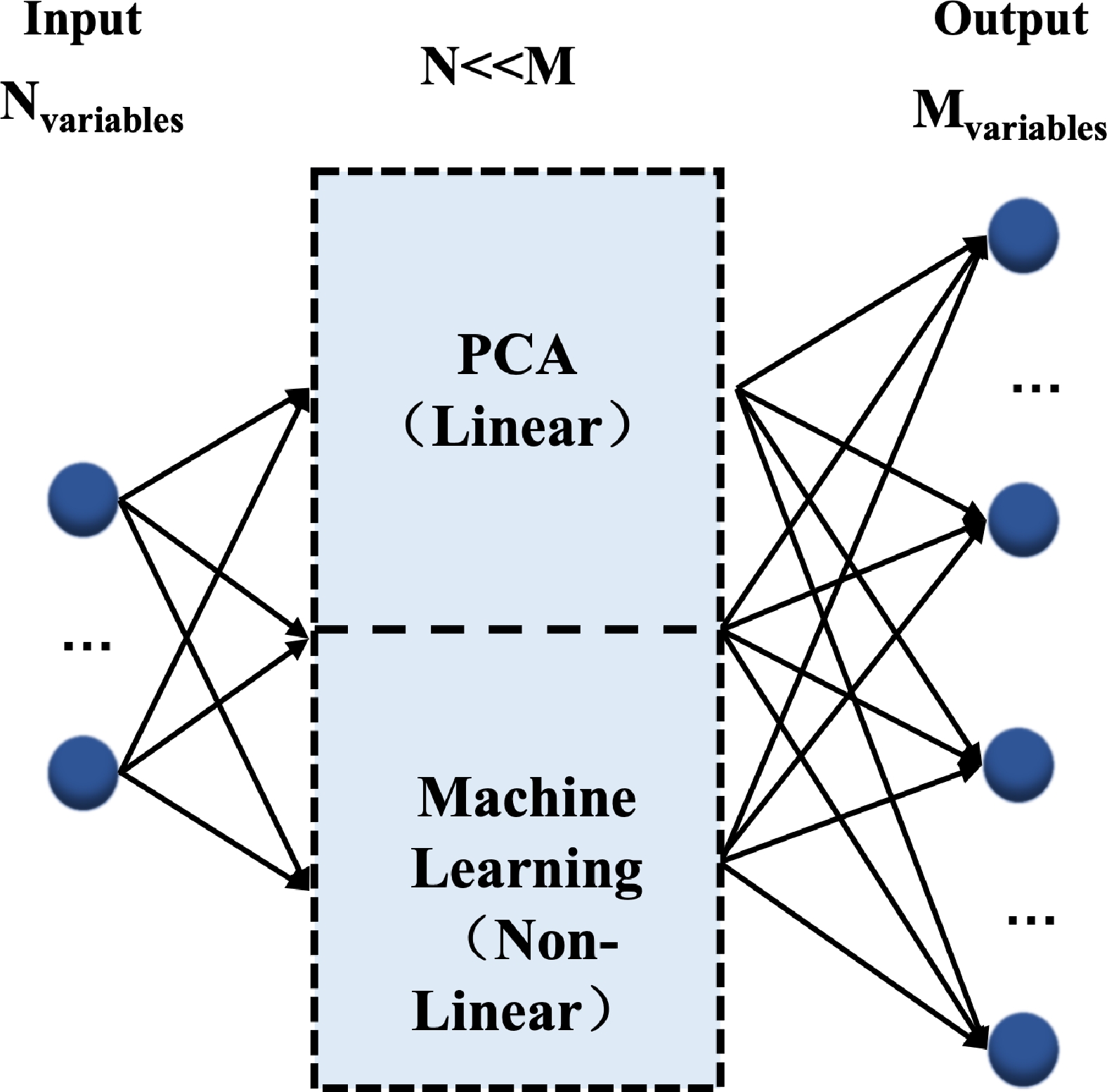
Figure 1 is a schematic of this essential idea for such an extension. Originally, the full spectral information of a vector with M elements may require M independent simulations. However, we can perform only N simulations (N could be much smaller than M and be a subset of M), and methods such as PCA or ML are performed to transform/extend this subset with N variables to the full vector with M variables. The advantages of such an extension are that 1) it is computationally efficient, and 2) the transform performed within the same parameter domain could be more stable because the variables have the same unit and similar values. Thus, we refer to such a procedure as the data/information “compression” during model development and that the forward-fast model performs multiple “extensions”. In the previous studies, such compression is performed for the monochromatic radiances in a mostly linear manner using the PCA (Liu et al., 2006), noting that there is still obvious potential for further improvements in other variable domains and for other extension methods.
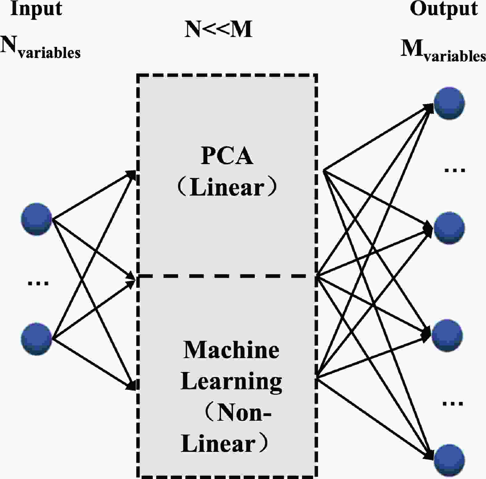
Figure 1. Schematic of the essential idea for data/information compression used in our model. The left dark blue circles can be understood as the chosen representative variables, and the right ones are the resulting complete variables.
In the framework of the PCA method, suppose we have a variable X (e.g., radiances at different wavenumbers) that contains M elements, and we have pre-calculated results from P different atmospheres. Thus, a full radiance matrix with a size of P × M can be established as XP×M, and when the P atmospheric conditions are large and with adequate representation, XP×M can be transformed in the form of its principal components (PCs), i.e., PCM×M. Thus, a new vector, VM, for monochromatic radiances of a new atmospheric profile can be expressed as the sum of these pre-calculated PCs and their coefficients, i.e., PC scores. Because the PCs capture spectral variations of radiances from one spectrum to another, at first, a few tens or hundreds for PCs (e.g., l PCs) are sufficient to give an accurate VM. Meanwhile, the corresponding PC scores Wl can be given by:
Here, the T means the matrix transposition, VN is a subset of VM, and PCl×N is the first l PCs with only the corresponding N elements. Thus, based on the PCA model, we have the following:
where VN is the subset on the left side of Fig. 1, and VM is the full set on the right. Thus, for any new profiles, we only need to calculate VN, and the full set of variables can be given by Eq. (2) with the pre-calculated PCl×M.
In other words, the PCA method uses a linear transformation to extend the VN to VM, and a large amount of spectral information is stored in the pre-calculated PCs. Meanwhile, ML methods are widely used to reveal complex relationships among different variables, so such an extension can also be performed by an ML-based model. In the ML model, VN and VM are understood as the predictor and predictand, respectively:
This study considers the NN as our example of a typical ML model. We use a fully connected two-layer NN model. The input layer consists of N neurons, i.e., the same set as the PCA method, and the output layer consists of M neurons, i.e., the full set of variables.
In the traditional PCA-based RT models, the abovementioned procedure is applied to the monochromatic radiances once, and VM is the vector with M monochromic radiances. Meanwhile, gas transmittance based on an LBL model is also tedious and time-consuming because it is needed for each absorbing gas, each wavenumber, and each atmospheric layer. Thus, we also adopt the PCA/NN method to gas transmittance calculations, and gas transmittances at different layers and different wavenumbers are treated as a one-dimensional vector to be considered together by one compression calculation. Thus, only a small fraction of gas transmittances and radiances are needed. Because the number of gas transmittance calculations is significantly reduced, interpolations based on pre-calculated gas absorptions at typical cases become possible and take much less computational storage.
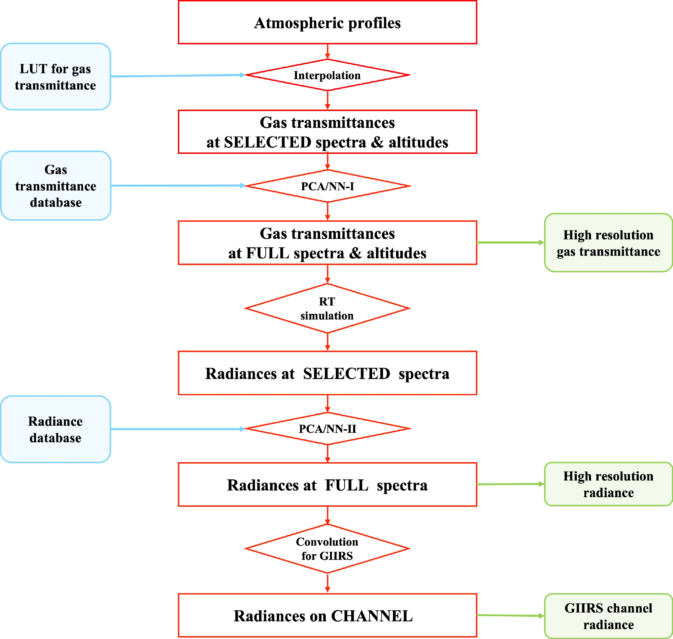
Thus, the overall procedure of our fast model is summarized in Fig. 2. The left part (Blue) indicates the pre-calculated or pre-trained datasets used, and the right part (Green) represents the outputs and byproducts that our model can produce. Besides the channel-based radiances as the final output, such a model can yield full monochromatic gas transmittances and radiances as well, which means it could be easily modified to serve simulations of other instruments within a similar spectrum. The middle red part shows the five major steps, corresponding to the five rhombi in the figure, for our simulator.
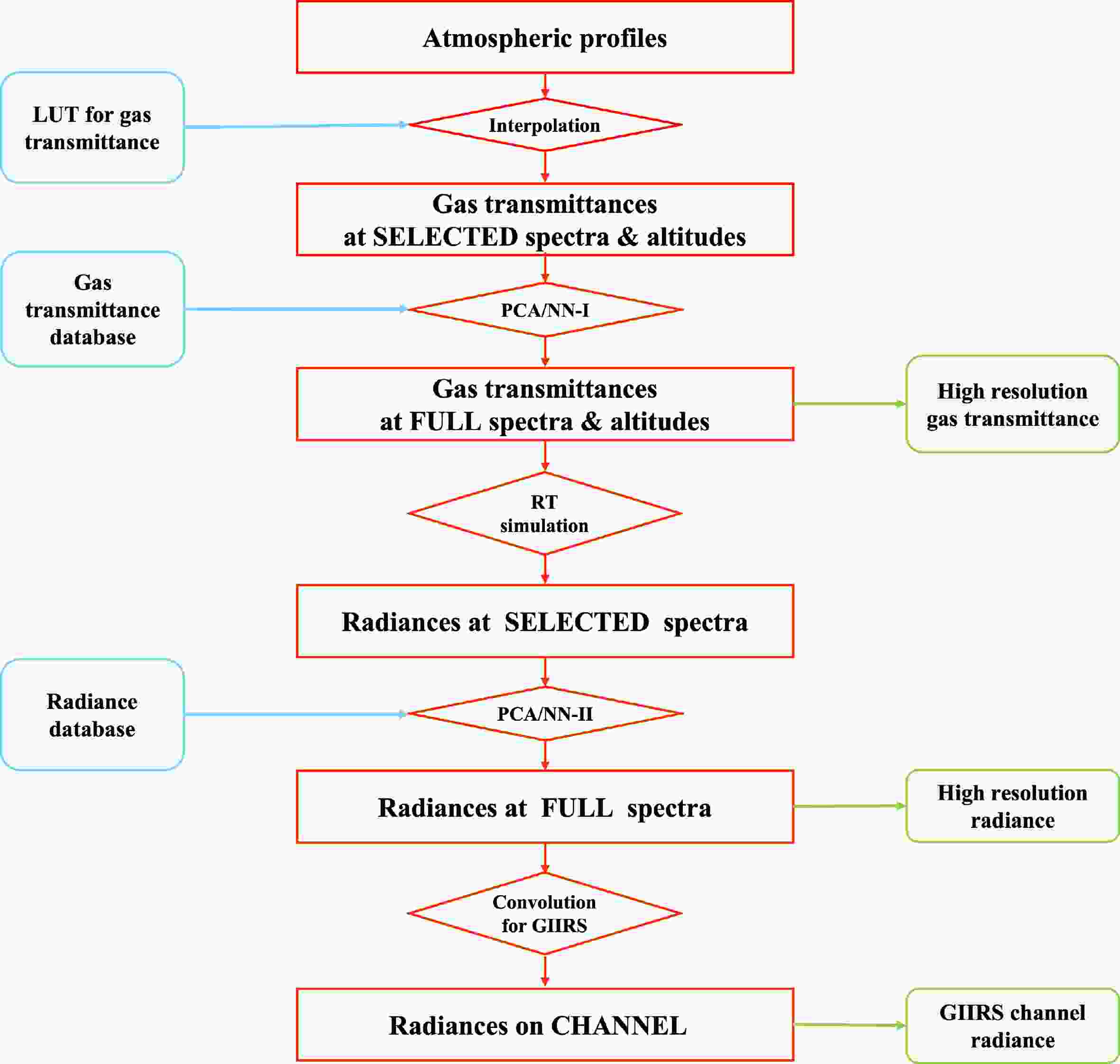
Figure 2. Flowchart of our hyperspectral resolution fast radiative transfer model. Red indicates the major computational procedures, and the five rhombi indicate the particular calculations. Blue indicates the pre-calculated or pre-trained datasets generated during model development. Green is for possible outputs of the model.
First, the gas transmittances at a very small fraction of wavenumbers and altitudes (in the form of particular pressures and temperatures), e.g., Ntrans, are calculated by interpolation, i.e., getting TN-trans. Notice that the transmittances are calculated independently for each gas (H2O, O3, and CO2). Because the pressure and wavenumber domains are combined for compression/extension, the interpolation is only performed for different temperatures of a given/new atmospheric profile. To ensure an accurate interpolation, we prepare gas absorption coefficients at each pressure and wavenumber (Ntrans for each gas) with temperatures ranging between 160 and 310 K, with a step of 2 K.
Second, those Ntrans typical gas transmittances are extended to full transmittances (Mlayer × Nwvn) at typical wavenumbers (Nwvn) and for all pressure layers (Mlayer) using the PCA/NN method, and Nwvn is only the number of typical wavenumbers for the following RT simulations. Thus, instead of performing a full set of Mlayer × Nwvn simulations for the gas transmittance, only Ntrans are needed in the previous step. Such treatment would not only reduce the computational burden but also require a much smaller pre-calculated database for interpolations. Thus, our model includes this efficient gas transmittance part using the atmospheric profile as the only input, so it has the advantage of avoiding an extra-complicated gas absorption scheme.
Third, with the full gas transmittances and atmospheric profile, rigorous RT simulations can be performed at those Nwvn representative wavenumbers to give monochromatic radiances (IN-wvn). In this study, we consider only the clear sky conditions, so a standard Schwarzschild Equation and its solutions are enough. If the method is extended to cloudy or hazy atmospheres with multiple scattering, this RT solver could be replaced by other models, such as the discrete ordinate method or others.
Fourth, the second extension is carried out to extend those typical radiances IN-wvn to monochromatic radiances (IM-wvn) in the full spectrum (assuming there are Mwvn monochromatic wavenumbers for the simulation). This step is similar to the traditional PCA-based ones but performs the extension with either the PCA or NN method.
Finally, the resulting high spectral radiances IM-wvn can give the channel-based radiance Ichannel by considering the channel spectral response functions (SRF) in the form of convolution. With the monochromatic radiances given from the above step, this independent calculation makes our model highly convenient to apply to instruments of similar kinds by only updating corresponding SRFs. Mathematically, the convolution can be performed together with the previous PCA model by multiplying the PC and convolution SRF matrices (Liu et al., 2006).
Thus, by using PCA/NN twice, the numbers of gas transmittance and RT simulations, respectively, are both reduced. Three pre-calculated datasets can be prepared during model development, which take little computational time and memory during model application. The following session provides additional details of three databases.
We consider the GIIRS onboard the Fengyun-4A as an example of model development. The GIIRS includes two bands, i.e., the Long-Wavenumber Band (LWB) ranging from 680 to 1130 cm–1 (or 8.85–14.71 µm) and the Middle-Wavenumber Band (MWB) ranging from 1650 to 2250 cm–1 (or 4.44–6.06 µm), noting that both of them have a channel spectral resolution of 0.625 cm–1. Thus, the two bands have 721 and 961 channels, respectively (Di et al., 2018). The LWB is mainly designed for atmospheric temperature and ozone soundings, and the MWB is used primarily for atmospheric humidity soundings. By using a basic spectral resolution of 0.025 cm–1, we consider 18 161 and 24 161 wavenumbers to fully cover the GIIRS LWB and MWB, respectively, which are the Mwvn values in this study. The GIIRS onboard the Fengyun-4B satellite was launched in 2021. The FY-4A/GIIRS only uses the wavenumber range of 700–1130 cm–1 for the observed LWB, and FY-4B/GIIRS extends the observation range to 680–1130 cm–1. The sensitivity of FY-4B/GIIRS is also improved to be suitable for detecting the changes in various atmospheric trace gases (Li et al., 2022b; Zeng et al., 2022, 2023). Due to similar instrument parameters, our model is expected to be applicable to both GIIRSs onboard the Fengyun-4A and Fengyun-4B. At the same time, it is noteworthy that finer spectral resolution would further enlarge the efficiency gain of our model because it would require little additional effort for PCA/NN-based models.
It follows that both a transmittance and monochromatic radiance database for PC calculations and NN training should be prepared. The SeeBor Global Profile database (v5.0) is chosen as the representative atmospheric profile for the training set (Borbas et al., 2005). Created at the Cooperative Institute for Meteorological Satellite Studies (CIMSS) of the University of Wisconsin-Madison, it consists of global atmospheric profiles of temperature, moisture, and ozone at 101 vertical pressure levels for clear-sky conditions. The profiles are generated from several sources, including NOAA-88, an ECMWF (European Centre of Medium-Range Weather Forecasts) 60-L training set, TIGR-3, ozone sondes from eight NOAA Climate Monitoring and Diagnostics Laboratory sites, and radiosondes from 2004 in the Sahara Desert. Three thousand profiles are randomly chosen from the datasets for our model development. For model validation, an independent dataset from the ECMWF global profiles (EC-Global) (Chevallier et al., 2006; Matricardi, 2008) is selected. The testing dataset contains 80 profiles generated at the European Centre of Medium-Range Weather Forecasts (ECMWF) by Matricardi (2008), which are sampled from a large profile database described in Chevallier et al. (2006). These profiles have been widely used for genegenerating and validation RTTOV coefficients for various satellite sensors at ECMWF for satellite data assimilation (Saunders et al., 2018) and CRTM transmittance training. The complete independence between our training (1000 profiles) and testing (all 80 profiles) datasets ensures the fidelity of validation, as indicated in Fig. 3. The LBLRTM (Line-By-Line Radiative Transfer Model) version 12.9 developed by AER (Clough et al., 2005) is used for transmittance calculations, and the HITRAN 2012 spectroscopic database (Rothman et al., 2013) is used as the source file of the gas absorption lines, and the Schwarzschild Equation is used for radiance simulations. Figure 3 illustrates some examples of atmospheric temperature and water vapor profiles of the training and testing datasets. Clearly, a wide range of variations is needed to ensure representativeness, and the testing dataset range is mostly within the training one.
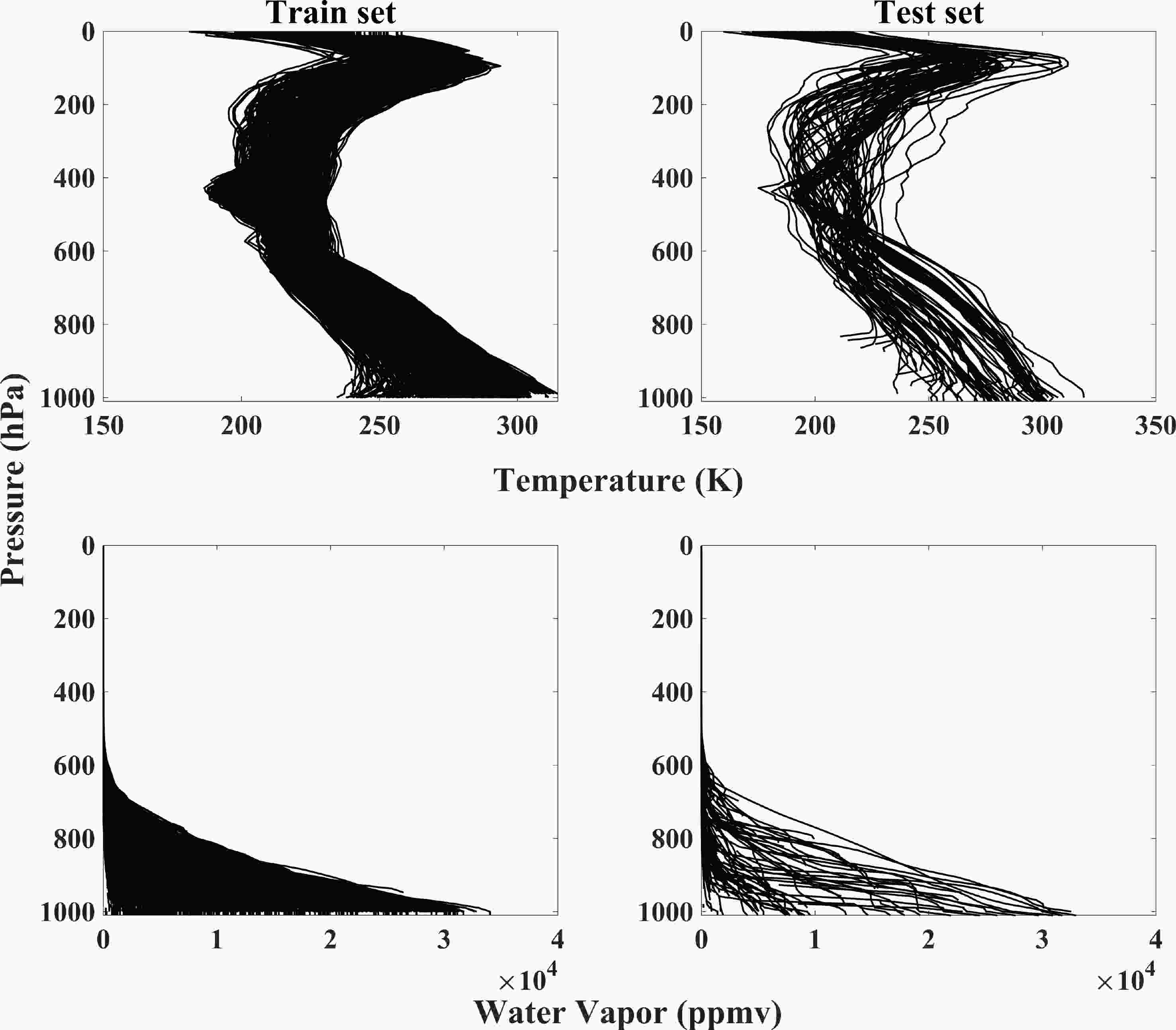
Figure 3. Examples of temperature and water vapor profiles in the (left) training dataset (from the SeeBor Global Profile database) and (right) independent testing dataset (from the ECMWF global profile database).
-
During model development, the gas absorption/transmittance and radiance datasets are calculated in advance (the blue boxes in Fig. 2), and representative elements are selected for the two PCA/NN simulations. This section details feature selection and the two PCA/NN procedures. Note that the datasets must be built backward during model development because the spectral information (from radiances to gas transmittances) is compressed to a minimum. The representative variables are also chosen backward among the necessary ones.
-
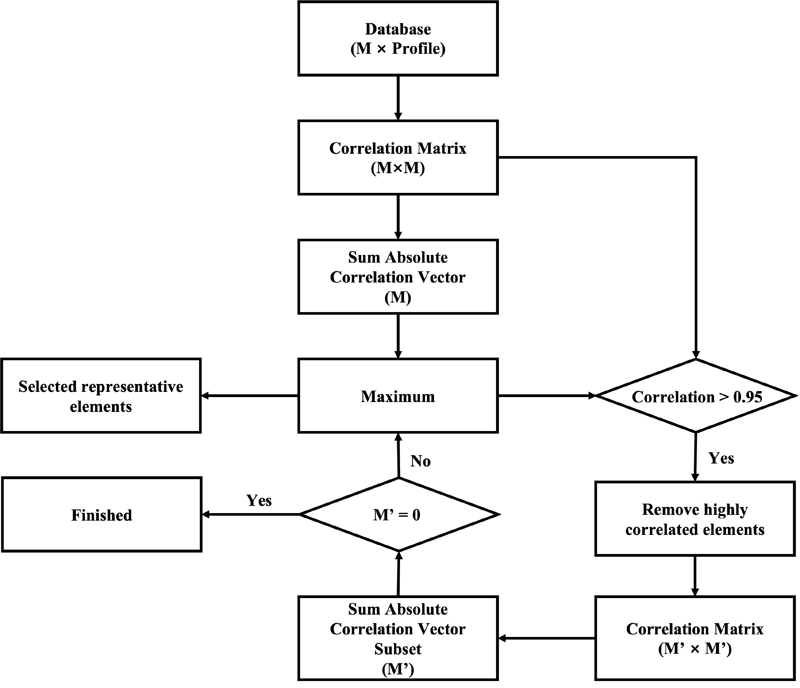
For the radiance domain compression, the monochromatic radiances best suited for the prediction of others should be chosen first. Both Liu et al. (2006) and Liu et al. (2020) have developed methods to choose representative radiances for the PCA-based simulations, and a more straightforward one is developed for our model. As shown in Fig. 4, the selection is mainly based on the correlations among the full monochromatic radiances. If the full set of radiances contains a total of M elements with values from many different atmospheric profiles, the correlation matrix of the radiances can thus be obtained, which indicates the linear correlations among different elements. Then, the sum of the absolute values for each row/column can quantify the correlation of each element with all the other elements, and it can be expressed as a vector with M elements. Larger absolute values indicate that the elements have stronger correlations with other elements and correspond to more informative radiances. Thus, the element that gives the largest summation is chosen first, and all other elements that have high correlations with the selected one would be eliminated from the chosen list (because the selected one well-represents them). We consider a correlation criterion of 0.95 for this step. After the first selection and removal, the correlation matrix of the remaining elements and the absolute value summation vectors are recalculated, and the chosen procedure is repeated until all elements are either selected or eliminated. Meanwhile, a small fraction of elements that give relatively larger errors is added to the representative dataset. This procedure is performed for both transmittances of different gases and monochromatic radiances.
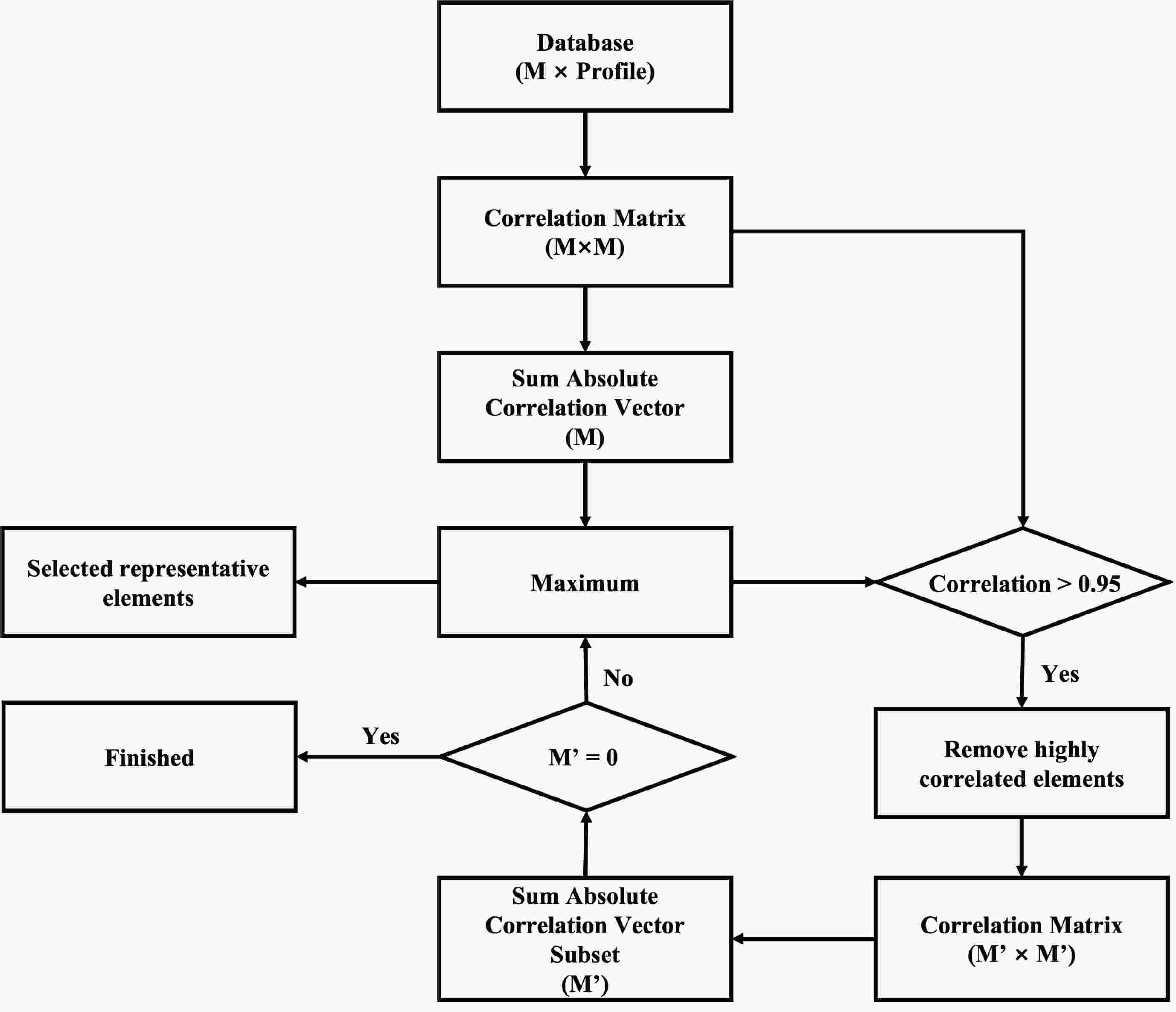
Figure 4. Procedure to choose the representative elements based on their correlations among different elements.
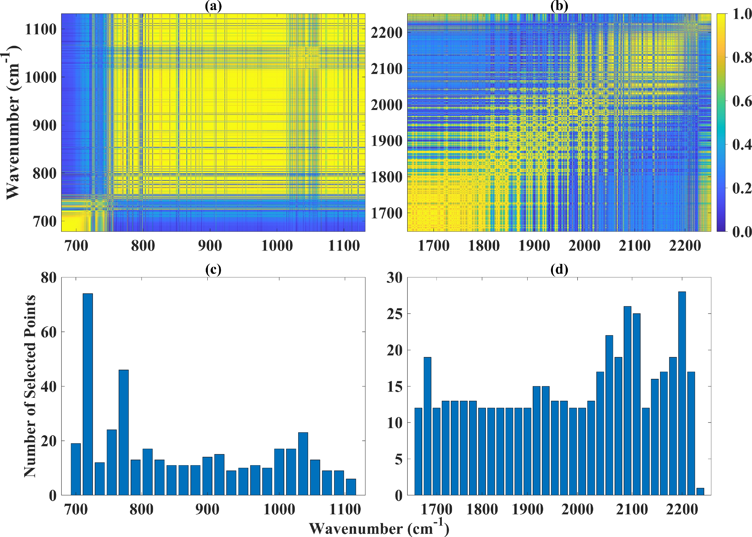
Figure 5 illustrates the corresponding results for the LWB (left panels) and MWB (right panels). The upper panels give the absolute values of the correlation coefficients among the monochromatic radiances. Higher correlations (yellow) are noticed among the independent gas absorption wavenumbers, e.g., carbon dioxide within the 680–1000 cm–1, ozone within the 700–1050 cm–1, and water vapor within the 1500–2000 cm–1 range. Through the correlation distributions and the feature selection mentioned above, we select 440 wavenumbers for GIIRS LWB (among 18 161, i.e., 2.4%), and 650 of these are selected for the MWB (among 24 161, i.e., 2.6%); their distributions in the spectrum domain are given in the bottom panels. The chosen wavenumbers are, for the most part, evenly distributed within the spectrum, with more elements chosen between 700 and 800 cm–1 and 2000 and 2200 cm–1 (the strong absorption spectral range), yielding a selected spectral set that is more representative.
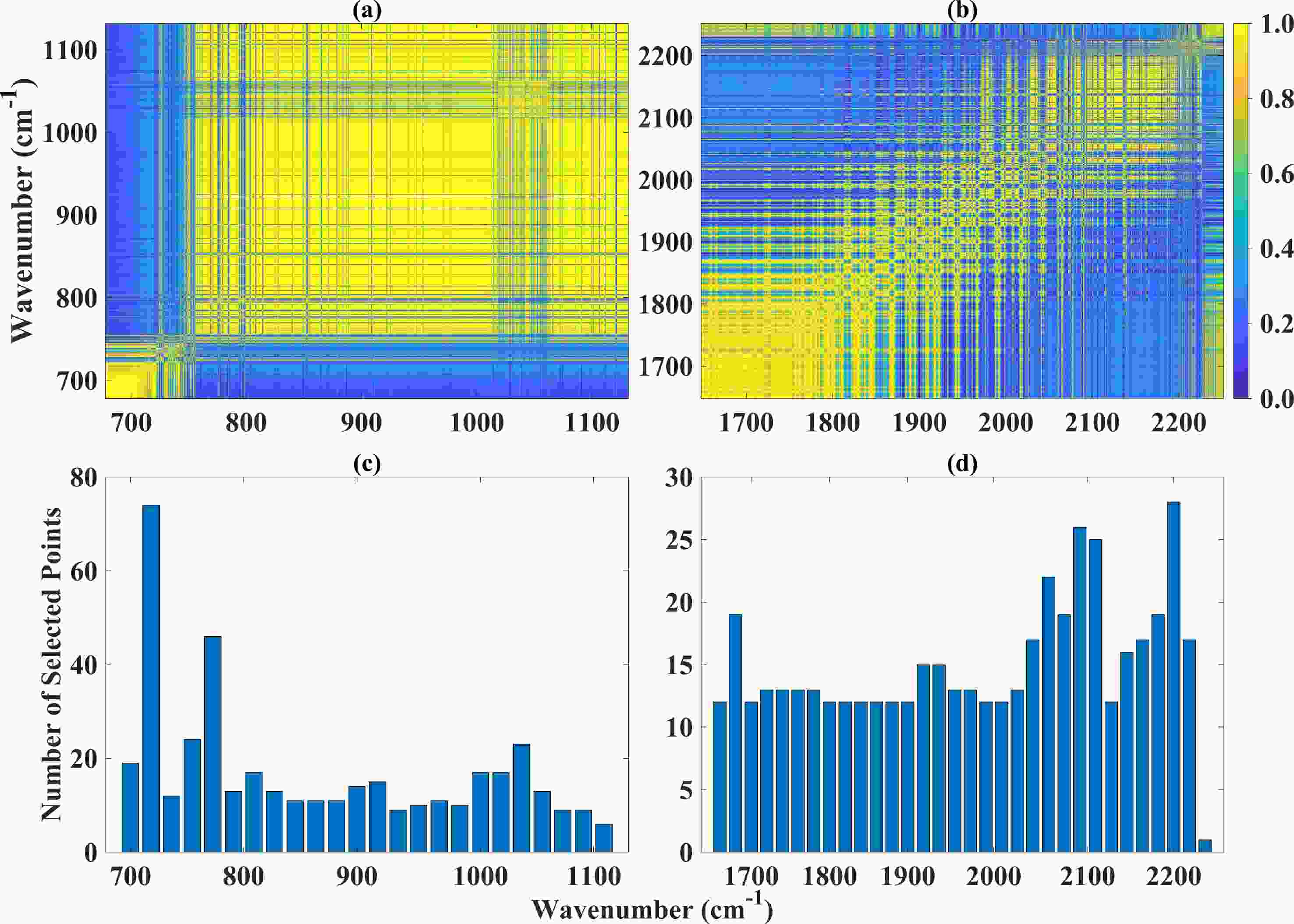
Figure 5. (top) Correlation coefficients between monochromatic radiances within each spectrum and (bottom) spectral distributions of numbers of selected representative wavenumbers.
Figure 6 shows the summations of the correlation coefficient absolute values for each wavenumber, which are key criteria for the feature selection, noting that the features are rearranged in increasing order. The summation is normalized by dividing the total number of wavenumbers within each spectrum, ensuring a value between 0 and 1. For the LWB, over half of the wavenumbers show summations of ~0.8, indicating redundant information among many monochromatic radiances, as the summation slowly decreases to ~0.2. The right panels show the density distributions among the correlation summation domain, and clearly, radiances with higher summations are less likely to be chosen. The results for MWB have slightly different summation variations, i.e., over 90% of points have summations over 0.4, and similar distribution features are noticed. Overall, approximately 2% of the points are chosen when the summation is over ~0.5, and less than 10% is enough when the summations are relatively small.
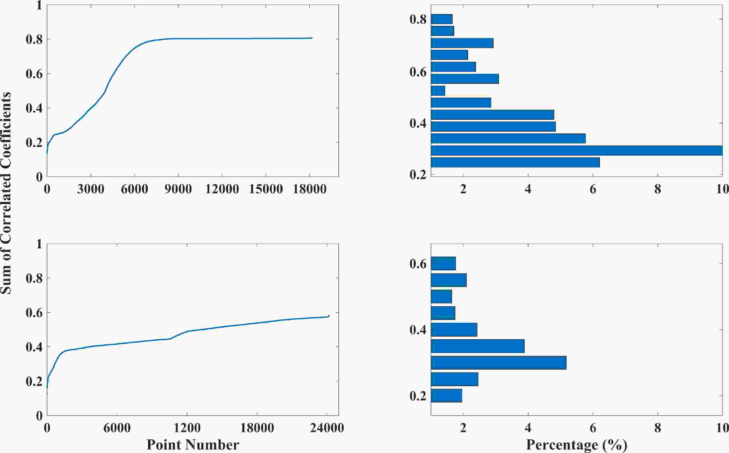
Figure 6. The rearranged sum of correlation coefficients of the monochromatic radiances and corresponding distribution probability of the selected representative wavenumbers.
-
Unlike the monochromatic radiances that are functions of only the wavenumber, the gas transmittances/absorptions are in both atmospheric and spectral domains. Since there is clear overlapping information in both dimensions, they are treated together, i.e., gas absorption coefficients at each pressure level and each wavenumber are consolidated into a whole dataset. The wavenumbers (only the selected ones for radiance PCA/NN, i.e., Nwvn = 440 and 650 for LWB and MWB, respectively) and pressure layers (100 layers between 0.005 and 1010 hPa) are fixed, so only the temperature difference is considered as a variable for dataset development. A similar feature selection is performed for each gas component. Considering that full gas transmittances at Nwvn wavenumbers and NLayer altitudes (a total of ~50 000) are needed, 1000–1500 representative absorption coefficients (Ntrans) selected for each absorbing gas for each compression in each band, which also constitute ~2% among all transmittances for this step. Note that the calculations are all conducted as logarithmic absorption coefficients.
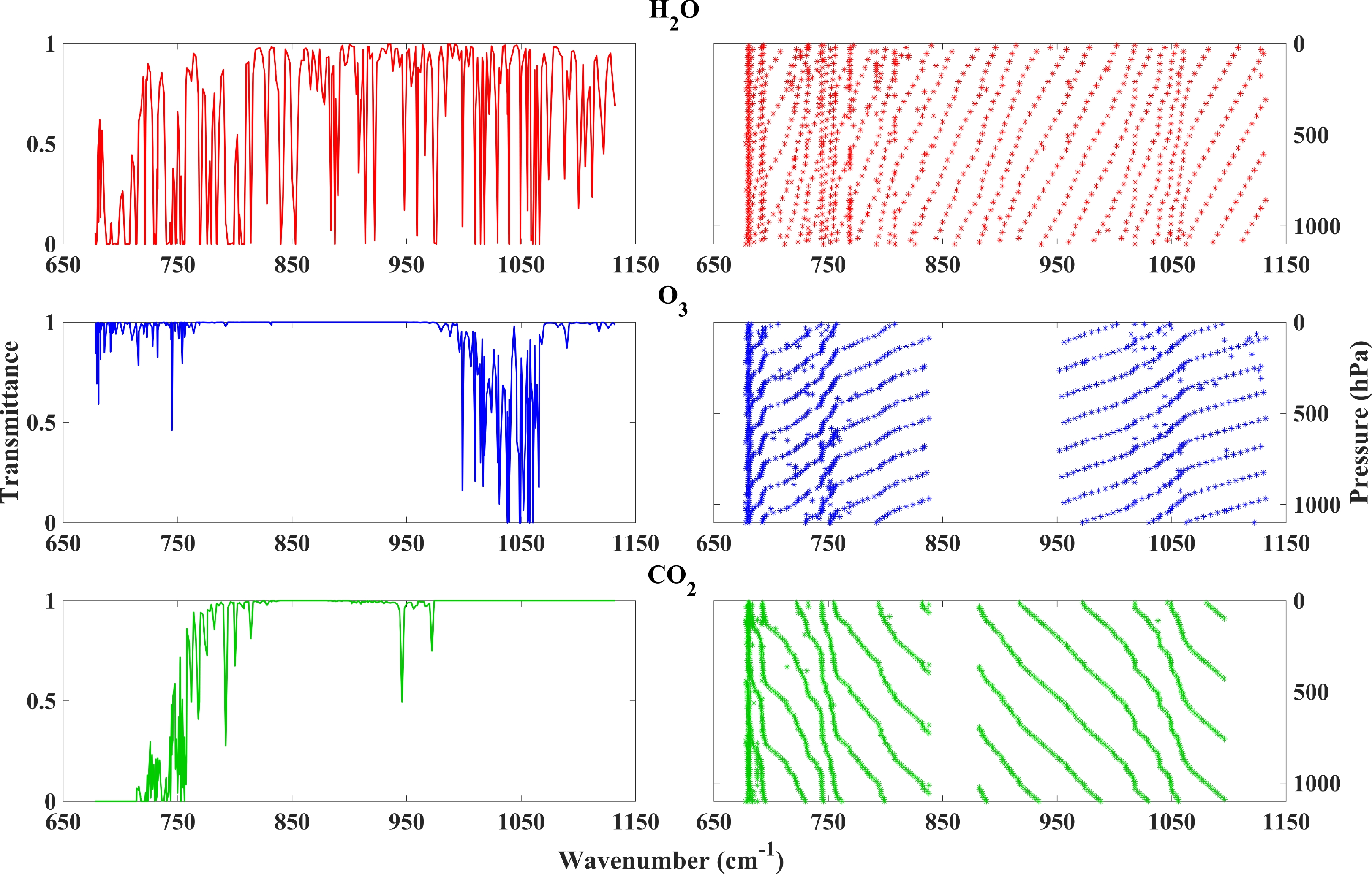
This study considers H2O, O3, and CO2 as absorbing gases, and examples of atmospheric transmittances in LWB are illustrated in Fig. 7. The results are for column transmittances from 1000 profiles and are given by 100 atmospheric layers. Only values at the selected wavenumbers are illustrated because the others are not needed for radiance simulations. In our model, those transmittances are also compressed and calculated by PCA/NN. The selected points within the spectral and atmospheric vertical height domain for gas transmittance calculations are given in the right panels. Due to the high correlations among the gas absorption coefficients, only a few elements are chosen based on our method, and more elements are added uniformly among the pressure and spectral domain to improve accuracy. There are more selections for spectral bands with strong absorption and fewer selections for spectral bands with transmittance close to 1, i.e., almost no absorption.
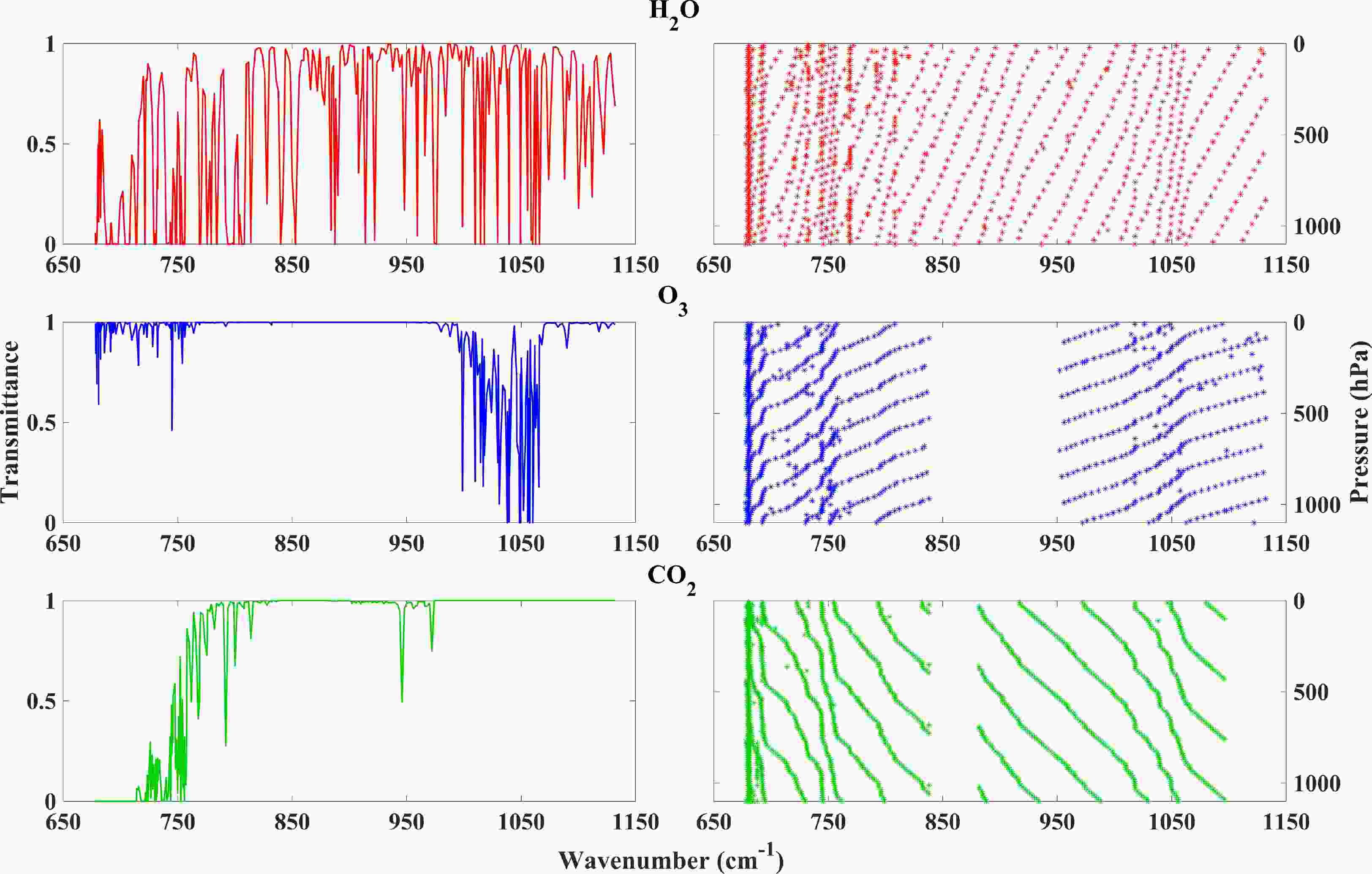
Figure 7. An example of column gas transmittances (left panels) for H2O, O3, and CO2 in the GIIRS longwave bands and the corresponding locations (right panel) of representative points selected in the pressure and spectral domain. Each dot in the right panels indicates one position with the given wavenumber and pressure, where the transmittance is chosen as our representative variable.
Lastly, only the gas transmittances at a highly compressed number of wavenumbers and atmospheric conditions are needed, i.e., those in the right panel of Fig. 7. Absorption coefficients for any new profiles are calculated by interpolation, which is given by pre-calculated, gas absorption coefficient look-up tables (LUTs). Because of the small number of transmittances required, such LUTs are small and can be easily implemented. Furthermore, each gas component is considered independent, and the interpolation can be performed quite accurately. The LUTs consider a wide range of temperatures from 160–310 K, with an interval of 2 K.
To summarize, Table 1 lists the specific parameters constructed for our model. The first three columns give the numbers required for full dataset simulations or for accurate LBL simulations, i.e., number of atmospheric layers (MLayer), number of full spectral wavenumbers (Mwvn), and their product (number of full gas transmittances, Mtrans). The remaining columns are for the numbers required for our spectral compressed simulations. From the above selections, we can get the set of representative spectra Nwvn that are much smaller than Mwvn, but carry the most useful information.
Band MLayer Mwvn Gas Trans
MtransComp-Trans ${{N} }_{\rm{trans} }$ Comp-Rad
${{N} }_{\rm{wvn} }$Comp-Trans Fraction Comp-Rad
FractionH2O O3 CO2 LWB 100 18 161 1 816 100 1000 1100 1500 440 ~ 0.1% 2.4% MWB 100 24 161 2 416 100 1100 1300 1200 650 ~ 0.1% 2.6% Table 1. Specific parameters of the new model for the GIIRS Long-Wavenumber Band and Middle-Wavenumber Band. “Comp” in the table represents the number used for our compressed variables.
For the PCA calculation, the PCs can be stored in advance from the results of our training atmospheric profiles and LBL simulations. This is done during the model development and is not repeated for model application. After testing, we selected the first 200 PCs to expand the data for both transmittance and radiation.
For the NN-based transmittance model, we set up a two-layer learning algorithm. The mean squared error and Rectified Linear Unit (ReLu) are used as the loss and activation functions, respectively, and the number of hidden neurons is set to 2000 (Glorot et al., 2011; Taylor et al., 2016; Le et al., 2020). Here, the activation function adds non-linear inputs to the neuron, and the ReLu is computationally efficient and accelerates the training convergence rate (Le et al., 2020). Similarly, the radiation-dimension model uses a three-layer ReLu model to account for the more complex relations among the monochromatic radiances, and the numbers of hidden neurons are set to 1000 and 2000, respectively. The number of iterations for both models was set to 2000, which is large enough to achieve stable results. Notably, many NN models with different variables and values were tested, and the value results mentioned above are closest to the accurate ones.
-
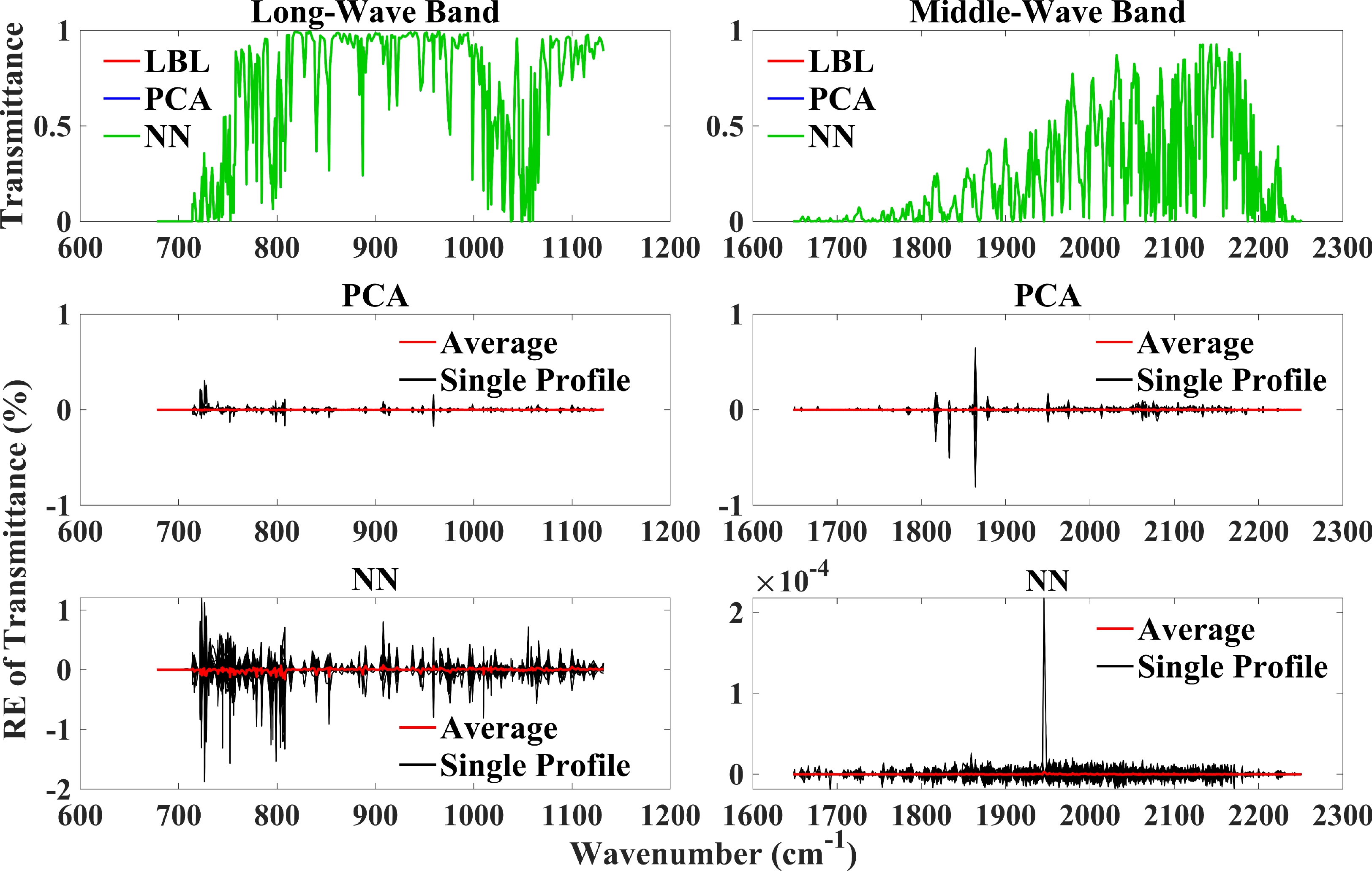
Figure 8 compares the column gas transmittances at the selected wavenumbers given by the LBL and our PCA- and NN-based simulations, which are the outputs for our first extension. Again, a testing dataset with 80 EC-Global profiles is used. The top panels are for the averaged transmittances, noting that both PCA and NN results closely agree with the LBL ones. The relative errors (REs) of the PCA-based and NN-based results are illustrated in the middle and bottom panels, respectively. The relative errors are defined according to the maximum transmittances within each spectral band, following the definition by Liu et al. (2020). The blue curves represent errors from each of the 80 EC-Global testing profiles, and the red ones indicate their average. The maximum REs for both models and both bands are under 1%, while most are under 0.1%, yielding average REs for each profile within ±0.2%.
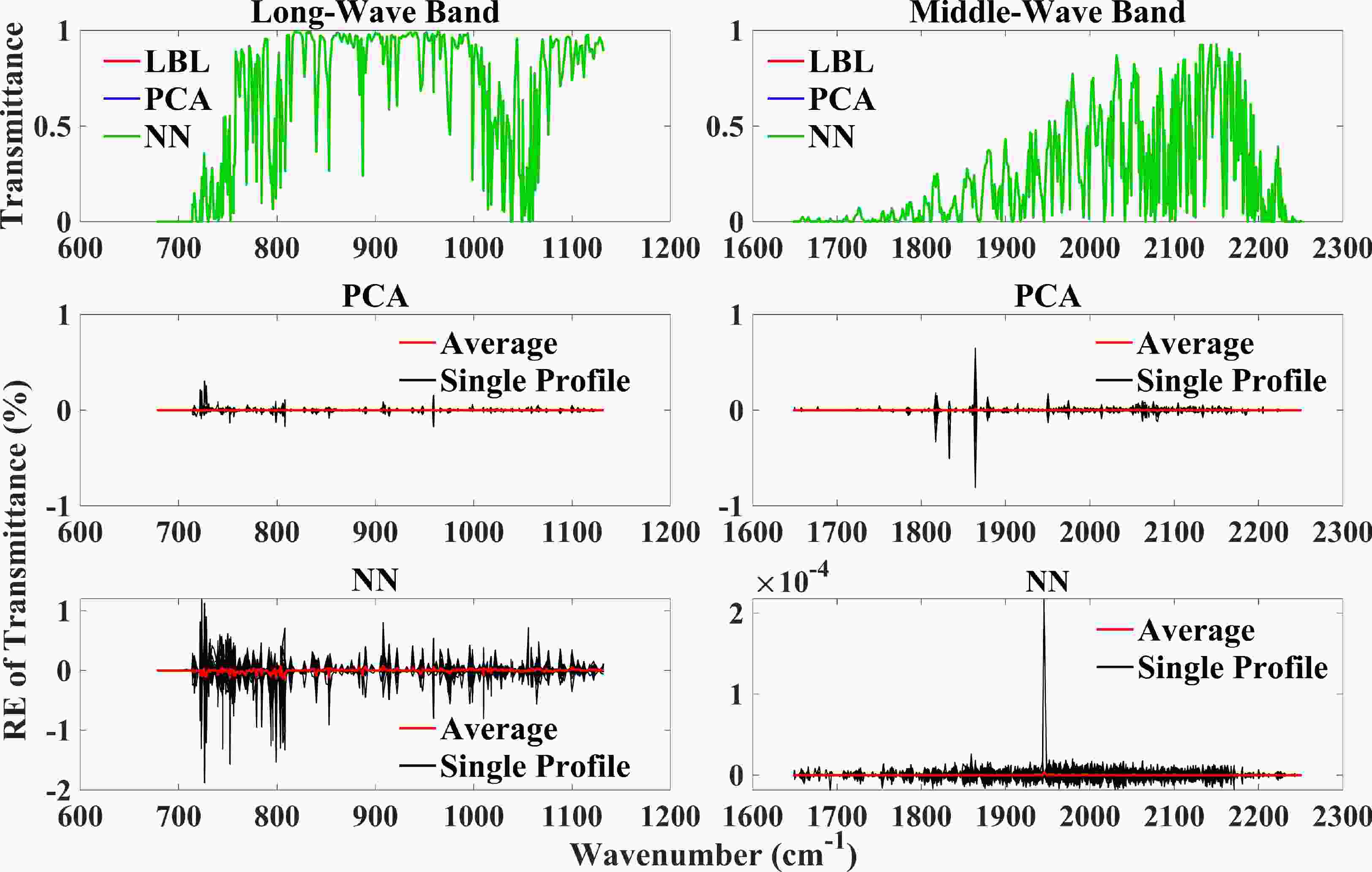
Figure 8. (upper) Averaged gas transmittances and their relative errors (RE) given by the (middle) PCA-based and (bottom) NN-based simulations compared with the LBL results at only the representative wavenumbers. The independent 80 EC-Global testing profiles are used for comparison here. The black curves are for the REs of each profile, and the red ones are the averaged REs.
Given accurate gas transmittances, rigorous radiative transfer simulations and radiance domain PCA/NN are performed to give the monochromatic radiances with a spectral resolution of 0.025 cm–1. Figure 9 compares the radiances within the two bands given by LBL, PCA, and NN models, and the results are also based on the EC-Global profiles. Again, the differences between LBL-based and PCA/NN-based results are hardly noticeable, and the monochromatic radiance differences are on the order of 10–5 W m–2 Sr–1 cm. Such accuracy is similar to those reported by previous studies (Liu et al., 2006; Le et al., 2020). The PCA-based results are slightly better in the MWB, while the NN-based model is better in LWB. Note that the bias and the mean differences contained here include those from the two PCA/NN simulations as well as the absorption coeffeicient interpolation.
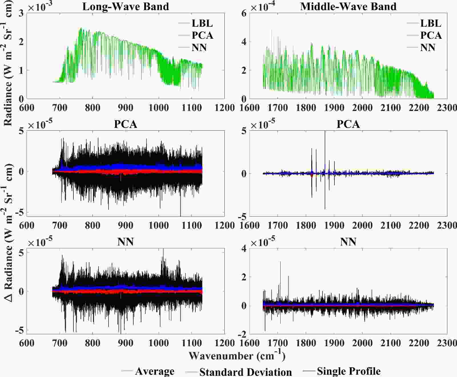
Figure 9. Similar to Fig. 8, but for the averaged hyperspectral revolution radiance and radiance differences and standard deviations of PCA-based and NN-based results.
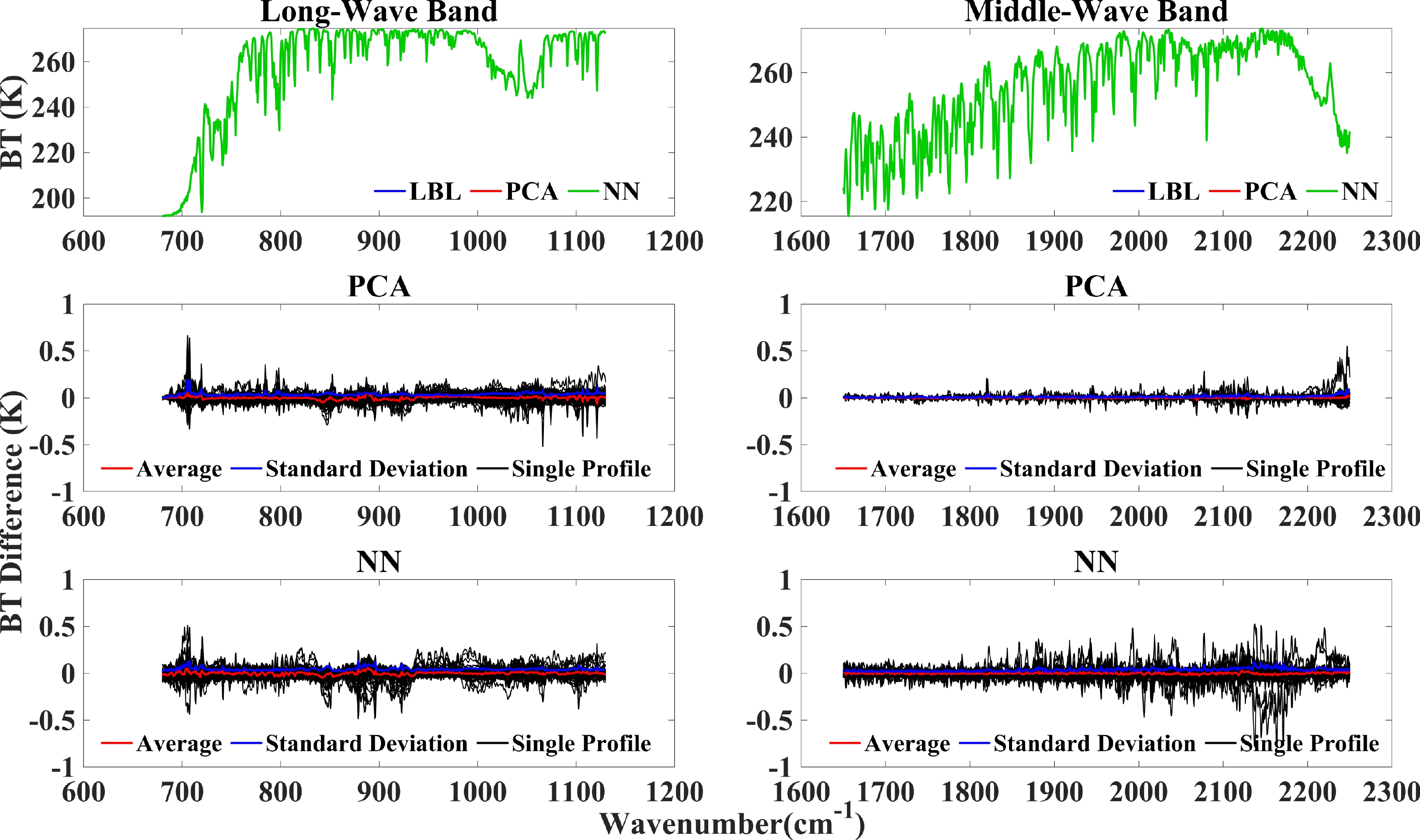
After the high-spectral-resolution monochromatic radiance is obtained, it is straightforward to perform a convolution to give the channel-based radiances using the GIIRS SRFs; the resulting channel BTs are shown in Fig. 10. Here, we apply the GIIRS SRFs, as reported by Di et al. (2018). As expected, the accuracy is significantly improved after the convolution because the errors in each wavenumber can cancel or offset one other. Most channel BTDs are within 0.5 K, and the averages are on the order of (or less than) 0.1 K. In the MWB, a few profiles have a larger error in the NN performance because the training set samples should have greater coverage (Le et al., 2020). Relatively larger BTDs are noticed in the strong absorbing regions, e.g., around 700 cm−1 and 2200 cm−1, which could be caused by multiple reasons. The errors from gas overlapping absorption and radiance simulations within the strong absorbing spectral regions may accumulate. Furthermore, the BT variations within these regions are more significant and more sensitive to the atmospheric profiles, and a larger number of the atmospheric dataset may be needed to further improve the model performance here (Kan et al., 2020). Also, more representative wavenumbers can be added within the region of larger errors in future development.
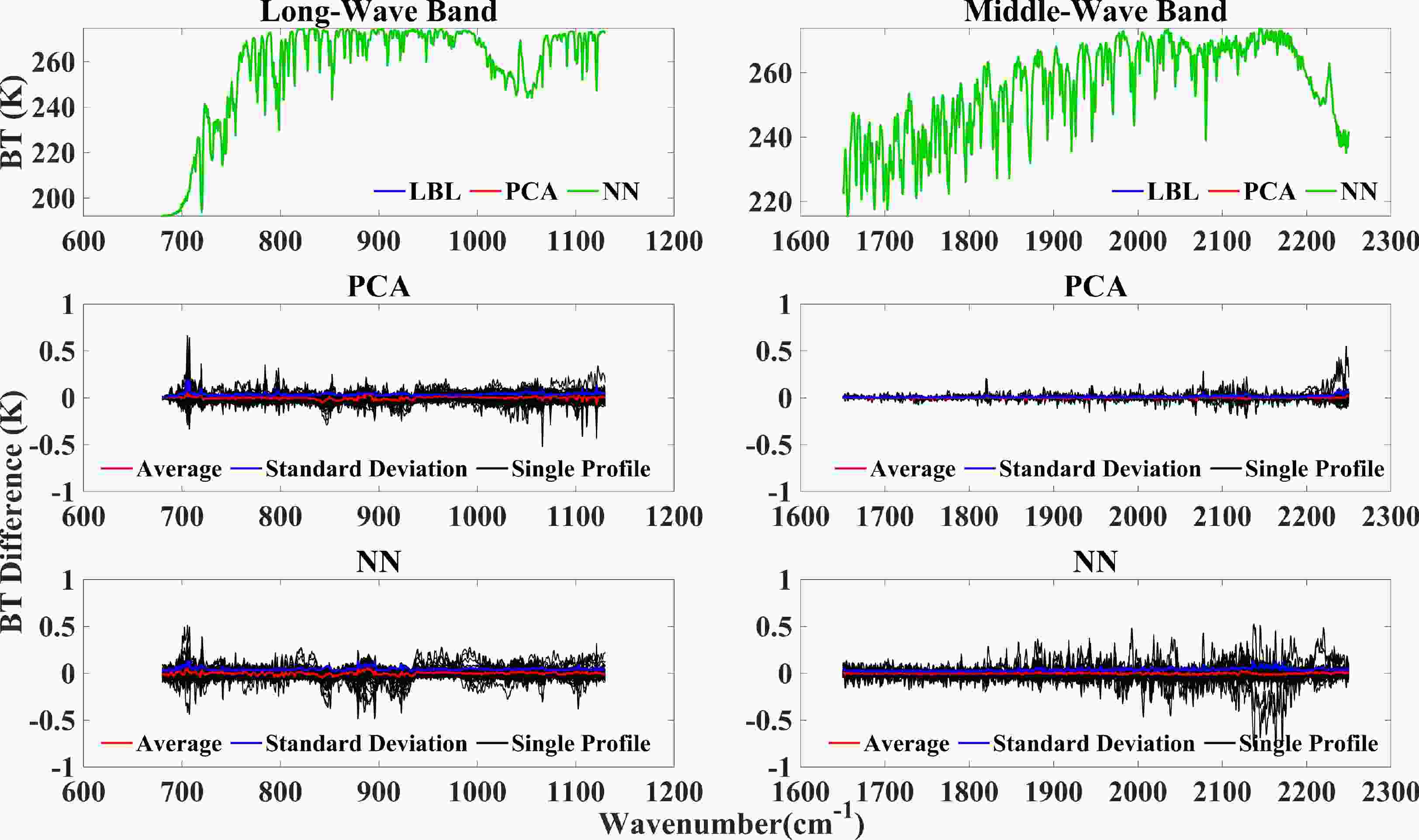
Figure 10. Similar to Fig. 9, but for GIIRS convolution brightness temperature (BT) and corresponding BT differences.
It becomes clear that the PCA/NN simulations can maintain computational accuracy with a greatly reduced number of independent simulations for both gas transmittances and radiances. Table 2 summarizes the computational efficiency by comparing the multi-domain compression model to the LBL model. Considering the influences due to differences among computer processors, only the orders of computational times in units of seconds used for each step (64-bit processors with a frequency of 2.4 GHz) are listed. For the transmittance calculations, when both PCA/NN methods and interpolation are used, a speedup of three orders is obtained. For the radiance simulations, the improvement is almost proportional to the reduction of the independent RT simulations. Also, this study considers only clear-sky conditions, so the independent monochromatic simulations are highly efficient. Thus, the overall improvement of the computational efficiency is roughly three orders of magnitudes.
Transmittance Radiance Total LBL-based Model (s) 102 100 102 Our Model (s) 10–1 10–2 10–1 Speedup 103 102 103 Table 2. Comparison of computational time between our model and the LBL model. The computational times are scaled to the nearest order of magnitude in units of seconds.
-
In summary, the multi-domain compression radiative transfer model established in this paper applies the PCA/NN method twice in the absorption coefficient and radiation dimensions, respectively, to accelerate the high spectral resolution RT simulations. Besides the conventional spectral compression on the monochromatic radiance domain, this study extends the PCA/NN method to gas absorption over the atmospheric and spectral domains, improving the computational efficiency and avoiding extra complicated transmittance schemes. It is found that the brightness temperature differences between our models and the LBLRTM are less than 0.5 K with an STD of less than 0.1 K, and the new models speed up their processing time by over three orders of magnitude. The PCA and NN achieve similar accuracies based on the same choices of the representative spectrum and pressures. Other machine learning methods may introduce improved accuracy, a premise to be tested in future studies. Also, the intermediate output transmittance dataset can be used directly in other models or algorithms, and our model can be extended to instruments with similar spectral coverage. However, the current model focuses only on the clear-sky conditions to avoid complexity due to multiple scattering from clouds or aerosols, noting that these factors will be included in our future development. We would also consider developing similar PCA/NN-based adjoint models (for Jacobians of radiances with respective to atmospheric variables) to extend our model applications for data retrieval and assimilation. More importantly, with excellent compactional accuracy and efficiency, the model is expected to better serve the development of GIIRS data retrievals and assimilations when the corresponding adjoint model is also developed.
Acknowledgements. We thank the Atomic and Molecular Physics Division, the Harvard-Smithsonian Center for the HITRAN dataset, and the Atmospheric and Environmental Research (AER) Inc for the LBLRTM model. This research is supported by the National Natural Science Foundation of China (Grant No. 42122038). The model simulations are conducted in the High Performance Computing Center of Nanjing University of Information Science & Technology.
| Band | MLayer | Mwvn | Gas Trans Mtrans | Comp-Trans ${{N} }_{\rm{trans} }$ | Comp-Rad ${{N} }_{\rm{wvn} }$ | Comp-Trans Fraction | Comp-Rad Fraction | ||
| H2O | O3 | CO2 | |||||||
| LWB | 100 | 18 161 | 1 816 100 | 1000 | 1100 | 1500 | 440 | ~ 0.1% | 2.4% |
| MWB | 100 | 24 161 | 2 416 100 | 1100 | 1300 | 1200 | 650 | ~ 0.1% | 2.6% |
 AAS Website
 AAS WeChat