


 DownLoad:


-
As an important component of the Antarctic climate system, landfast sea ice contributes more to sea-ice mass balance than drifting sea ice in East Antarctica (Giles et al., 2008). The existence of landfast sea ice reduces the energy exchanges between ocean and atmosphere, affecting regional atmospheric circulation. Numerical simulation is an essential means to predict the evolution of landfast sea ice, local weather conditions, and climate change in Antarctica (Zhao et al., 2022). In atmospheric numerical models, turbulent sensible and latent heat fluxes quantify the exchanges of heat and water vapor between the atmosphere and sea ice and determine the thermal structure in the lower atmosphere (Andreas et al., 2010), while turbulent momentum flux directly affects the wind speed near the surface (Best et al., 2011). Therefore, accurately describing turbulent fluxes is vital to the performance of atmospheric numerical models. However, in Antarctica, the evaluation of parameterization schemes for turbulent fluxes over the landfast sea-ice surface in numerical models is rarely investigated due to the limited observations (Liu et al., 2020a).
The bulk aerodynamic method based on the Monin-Obukhov Similarity Theory (MOST) is widely used for parameterizing turbulent fluxes in numerical models. However, different models show significant distinctions in simulating turbulent fluxes over a sea-ice surface, mainly for the different settings of stability functions and roughness lengths (Brunke et al., 2006; Radić et al., 2017). Stability functions, like the classic log-linear relations proposed by Businger et al. (1971) and Dyer (1974), are semi-empirical functions attained from field observation experiments in the mid-latitude areas (Lu et al., 2013; Ala-Könni et al., 2022). For the polar stable boundary layer, some stability functions are established mainly based on the data collected from the Surface Heat Budget of the Arctic Ocean (SHEBA) experiment, which lasted from 2 October 1997 to 11 October 1998 (Brunke et al., 2006; Grachev et al., 2007; Gryanik et al., 2020). For example, Grachev et al. (2007) proposed a set of stability functions for stable stratification by fitting the SHEBA observations, while Gryanik et al. (2020) improved these functions by considering the Prandtl number. However, few stability functions have been proposed to focus on the Antarctic boundary layer over the landfast sea-ice surface. Hence, the applicability of present stability functions in numerical models needs further validation for considering stratification effects over the Antarctic landfast sea-ice surface.
On the other hand, the settings of roughness lengths in models are quite different. Previous studies indicated that the roughness lengths over the sea-ice surface were determined by many complicated factors, including the types and age of sea-ice (Overland, 1985; Guest and Davidson, 1991), the snow over the sea-ice surface blown by the wind (Andreas and Claffey, 1995), the open water area (Andreas et al., 2005), and the preferential orientation of snow micro-reliefs (Vignon et al., 2017). Guest and Davidson (1991) suggested a typical range of the order of aerodynamic roughness length, 10−4−10−2 m, for the Antarctic sea-ice/snow surface. Andreas et al. (2005) proposed a parameterization for aerodynamic roughness length over the sea-ice surface. Then Brunke et al. (2006) developed a relation between aerodynamic roughness length and friction velocity, simpler than the equations in Andreas et al. (2005). Andreas et al. (2010) concluded that aerodynamic roughness length became a constant value, 2.3 × 10⁻⁴ m when the friction velocity reached 0.3 m s−1 in the SHEBA dataset. Based on the measurements at several Arctic sites, Andreas (2011) recommended estimating the aerodynamic roughness length according to the physical roughness length of the surface. Compared with the aerodynamic roughness length, the thermal and moisture roughness lengths present more complicated formulae (Andreas et al., 2010). However, for simplicity and practicability, many numerical models assume the roughness lengths over the sea-ice surface to be a constant, resulting in significant uncertainties in simulating turbulent fluxes (Brunke et al., 2006; Lu et al., 2013; Zhang et al., 2021).
Therefore, the stability functions and roughness lengths over the sea ice are essential for developing weather prediction and climate projection in the Antarctic and thus need to be evaluated and optimized by conducting more in-situ observations. In this study, five commonly used numerical models, including the Arctic Regional Climate System Model (ARCSYM), European Centre for Medium-Range Weather Forecasts Integrated Forecasting System (ECMWF-IFS), Community Atmosphere Model (CAM), Beijing Climate System Model (BCC_CSM), and Community Noah Land Surface Model with Multi-Parameterizations Options (Noah_mp) are selected for evaluating their performance in simulating turbulent fluxes over the Antarctic sea-ice surface by using the in-situ observation data collected at an Antarctic landfast sea-ice station from 8 April to 26 November of 2016. Then sensitivity tests are conducted to explain the model performance. At last, some characteristics of roughness lengths are presented. The remainder of this paper is organized as follows. The data and methods are described in section 2. We present the results in section 3, and a discussion and conclusions are given in section 4.
-
To investigate the energy budget at the Antarctic landfast sea-ice surface, we built an eddy-covariance (EC) observation system at a 3-m meteorological mast over the landfast sea-ice surface in the southern part of Prydz Bay. The site is located at 69°22′08.1′′S, 76°21′42.1′′E, in the northwest portion of Princess Elizabeth Land and to the east of Amery Ice Shelf. It is about 260 m from the nearest sea-ice edge. Based on the footprint analysis, 90% of the source area covered by the EC measurements is characterized by landfast sea-ice properties. The specific position of the site can be found in Fig. 1 of Liu et al. (2022). The observation period was sustained from 8 April to 26 November 2016. During this period, the landfast around the site increased from 0.5 m (in April) to 1.8 m (in November) in thickness and was covered by snow with an average depth of 0.1 m. Turbulent fluxes were measured by an integrated EC observation device called IRGASON, fixed at 2-m height. The sampling frequency of IRGASON was 10 Hz. The other slow response measurements installed at the meteorological mast included an infrared radiometer SI-111, a net radiometer CNR4, a temperature and humidity sensor HMP155, and a barometer CS106. The data collected during this field experiment were first published by Liu et al. (2020a), and detailed information on the measurements used in this study is displayed in Table 1. The 30-minute averaged turbulent fluxes used as reference values in this study are derived from the EC observation system. Similar averaging windows are suggested by Guo et al. (2011) for flux calculations in glaciated areas.

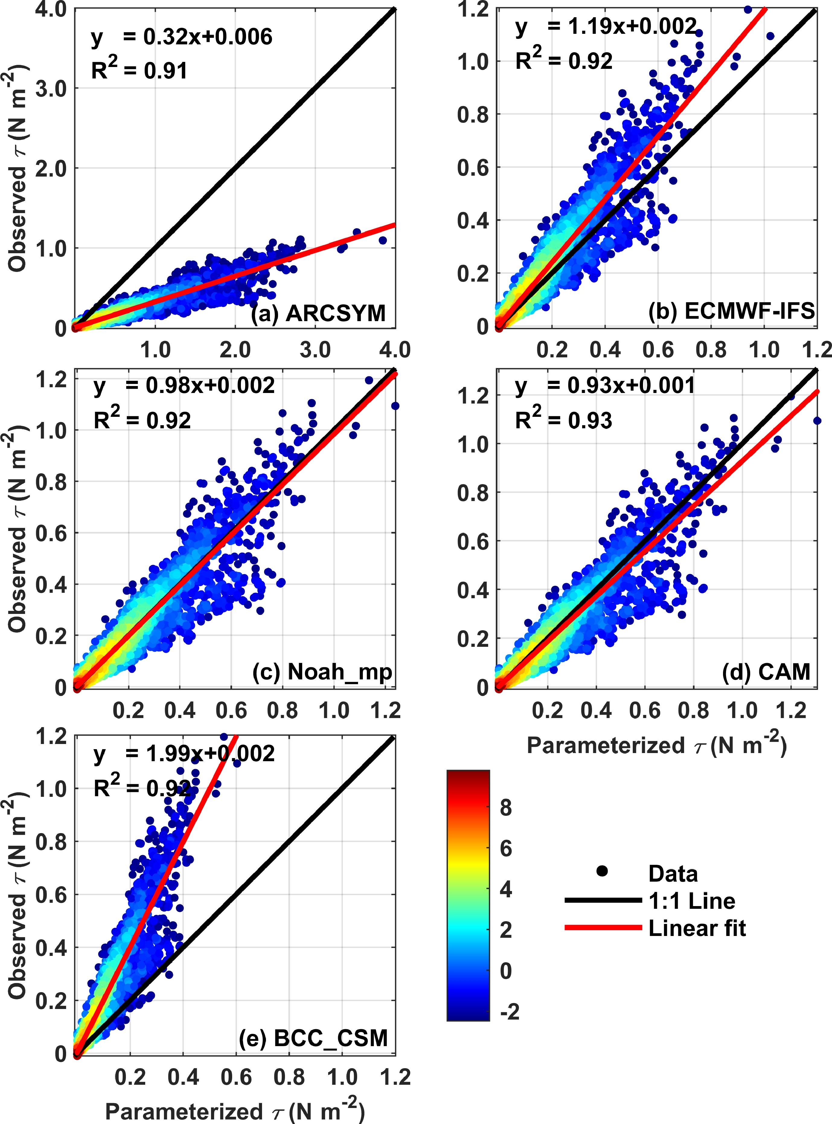
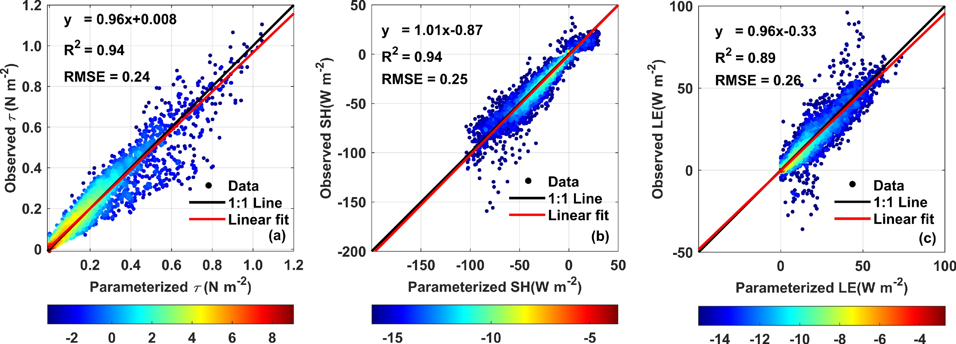
Figure 1. The comparison of the turbulent momentum flux (τ) between the simulation and observation. Panels (a)–(e) are the results derived from ARCSYM, ECMWF-IFS, Noah_mp, CAM, and BCC_CSM, respectively. Here, the points are colored by log2(p), where p is the occurring probability density of nearby points.
Instrument Measurement quantities Sampling rate Installation height SI-111 Surface temperature (Ts) 0.1 Hz 1 m HMP155 Air temperature (Ta); Relative humidity (RH) 0.1 Hz 2 m CS106 Atmospheric pressure (Pa) 0.1 Hz 0.5 m IRGASON Three-dimensional velocity (Ux, Uy, Uz); Sonic temperature (θv);
H2O Density ($\rho_{{\rm{H}}_2{\rm{O}}} $); Air Density (ρ)10 Hz 2 m Table 1. The key technical specifications of measurements used in this study.
-
The bulk aerodynamic method, which is usually used in numerical models, employs the MOST (Monin and Obukhov, 1954) to compute the turbulent fluxes by using conventional meteorological variables as follows:
where τ is the turbulent momentum flux, SH is the turbulent sensible heat flux, and LE is the turbulent latent heat flux (in this paper, upward turbulent fluxes are defined to be positive); Cm, Ch, and Cq are the bulk exchange coefficients for momentum, temperature, and moisture, respectively; U, θa, and qa are the wind speed, potential temperature, and specific humidity observed at the height of 2 m, respectively; θs and qs are the potential temperature and specific humidity at the surface from observation; ρ is the measured air density; cp (1004.07 J kg–1 K–1) is the heat capacity of air; Ls (2.835 × 10⁶ J kg–1) is the latent heat of sublimation; u*, θ*, and q* are the frictional velocity, potential temperature scale, and specific humidity scale, respectively.
The bulk exchange coefficients are the functions of the stability parameter and corresponding roughness lengths, as derived from:
where κ is the von Karman constant of 0.4 (Kim et al., 1987); z0m, z0t, and z0q are the roughness lengths for wind speed, temperature, and moisture, respectively; Ψm, Ψh, and Ψq are the stability functions for wind speed, potential temperature, and specific humidity, respectively, and
where Φm,h,q represents the corresponding dimensionless stability functions (the specific expression of Φm,h,q can be found in section 2.3), ζ is the stability parameter, which is defined as the ratio of the observation height (z) to the Monin-Obukhov length (L), and calculated from:
where g is the gravitational constant of 9.8 m s−2; hence, once roughness lengths and stability functions are determined, turbulent fluxes can be solved by Eqs. (1)–(9) iteratively.
-
In this section, we introduce the details of calculating turbulent fluxes in five numerical models.
-
The first model, ARCSYM, adopts a non-iterative method, i.e., the Cm ~ Rib and Ch, Cq ~ (ΔT, U) relations to calculate turbulent fluxes. The momentum exchange coefficient (Cm) is a function of z0m and the bulk Richardson number (Rib) in the surface layer and is calculated according to Louis’s (Louis, 1979) formulae:
here b equals 20, which is different from the Louis (1979) scheme; z0m depends on the snow depth (sd), i.e., z0m is set to be 6 × 10⁻² m for sd less than 5 × 10⁻² m but is reduced to 4 × 10⁻² m for deeper snow (Brunke et al., 2006). The exchange coefficients for moisture (Cq) and heat (Ch) are derived from empirical equations:
-
ECMWF-IFS is a comprehensive Earth-system model coupled with atmosphere, oceans, land, waves, and sea ice for weather forecasting. In ECMWF-IFS, z0m, z0t, and z0q over the sea-ice surface are all set to 1 × 10⁻³ m. ECMWF-IFS uses the classic functions from Paulson (1970; hereafter referred to as Paulson 1970) for unstable stratification:
and the functions from Holtslag and De Bruin (1988; hereafter referred to as HDB88) for stable stratification:
The corresponding dimensionless stability functions and roughness lengths are substituted into Eqs. (1)–(9) to derive the turbulent fluxes, which are also used in the following models.
-
Noah_mp, an extensive version of the Noah Land Surface Model with developed Multi-Physics options, is employed in the Weather Research and Forecast model (WRF), NCEP Climate Forecast System, and WRF-Hydro (The Weather Research and Forecasting Model Hydrological modeling system). In Noah_mp, z0m, z0t, and z0q over snow-covered surfaces are all set to 2 × 10⁻³ m. Paulson1970 is used for unstable stratification conditions, and the relations from Businger et al. (1971; hereafter referred to as B71) are used for stable stratification conditions (Niu et al., 2011):
Noah_mp makes quality control to eliminate fallacious values of ζ during the process of solving ζ:
Meanwhile, Noah_mp also quality controls Cm, Ch, and Cq as follows:
-
CAM, a reliable and well-documented global atmosphere model, is a major component of the Community Earth System Model (CESM) developed by the National Center for Atmospheric Research (NCAR). CAM sets z0m to be 2.4 × 10⁻³ m and predicts z0t and z0q according to the relations from Zilitinkevich (1970):
here, the kinematic viscosity of air υ = 1.5 × 10⁻⁵ m2 s−1 and a = 0.13 (Zeng and Dickinson, 1998). The novel expressions from Zeng et al. (1998; hereafter referred to as Z98) is used for stable conditions:
CAM employs the Paulson1970 functions for unstable conditions and the flux-gradient relations from Kader and Yaglom (1990; hereafter referred to as KY1990) for very unstable conditions:
-
BCC_CSM, a fully-coupled model with ocean, land-surface, atmosphere, and sea-ice components, was developed by Beijing Climate Center and used for phase six of the Coupled Model Intercomparison Project (CMIP6) (Wu et al., 2008; Wu, 2012; Xin et al., 2013). Based on the observational data of the fourth Chinese National Arctic Research Expedition (CHINARE 2010) and SHEBA, BCC_CSM sets superior stability functions and varying roughness lengths to improve the parameterization schemes over sea ice (Lu et al., 2013; Wu et al., 2019). BCC_CSM suggests Paulson1970 functions for unstable conditions and Z98 functions for stable conditions. z0m is set to be 1 × 10⁻⁴ m when the surface temperature (Ts) is less than −2°C and 8 × 10⁻⁴ m when Ts is greater than −2°C; z0t and z0q are predicted with the theoretical function by Andreas (1987):
where z0s refers to z0t or z0q, and the coefficients in Eq. (32) are listed in Table 2.
R* ≤ 0.135 0.135 < R* ≤ 2.5 2.5 < R* <1000 Heat (z0t/z0m) b0 1.250 0.149 0.317 b1 0 −0.550 −0.565 b2 0 0 −0.183 Moisture (z0q/z0m) b0 1.610 0.351 0.396 b1 0 −0.628 −0.512 b2 0 0 −0.180 Table 2. Values of coefficients for calculating the roughness length for heat and moisture
-
Figures 1–3 compare the simulated turbulent fluxes with the observations in terms of the slope and determination coefficient (R2) of the best-fit line via occurring probability density drawings. For the τ (Fig. 1), ARCSYM presents the greatest overestimated result, while BCC_CSM produces an obviously underestimated result. The other three models perform better than ARCSYM and BCC_CSM. The performance of Noah_mp ranks first among them, and ECMWF-IFS produces slightly underestimated values. For the SH (Fig. 2), the performances of the models are not as good as that of τ in ECMWF-IFS, Noah_mp, and CAM. Among the five models, ECMWF-IFS best fits the observation, but still produces an obviously overestimated result. BCC_CSM performs a little worse than ECMWF-IFS and is the only one that underestimates the SH. The slope of the best-fit line for ARCSYM is 0.58, which deviates from the reference line (1:1) most significantly compared with the other models. For the LE (Fig. 3), the models all overestimate it. It is clear that BCC_CSM fits the observations best, and the performance of BCC_CSM is much better than the other models. The slopes of the best-fit line for ARCSYM, ECMWF-IFS, Noah_mp, CAM, and BCC_CSM are 0.32, 0.57, 0.47, 0.50, and 0.96, respectively. It is noted that we have assumed the surface-specific humidity is saturated. Hence, the simulated LE is always larger than 0 W m−2. The R2 for any turbulent flux among the five models is comparable.
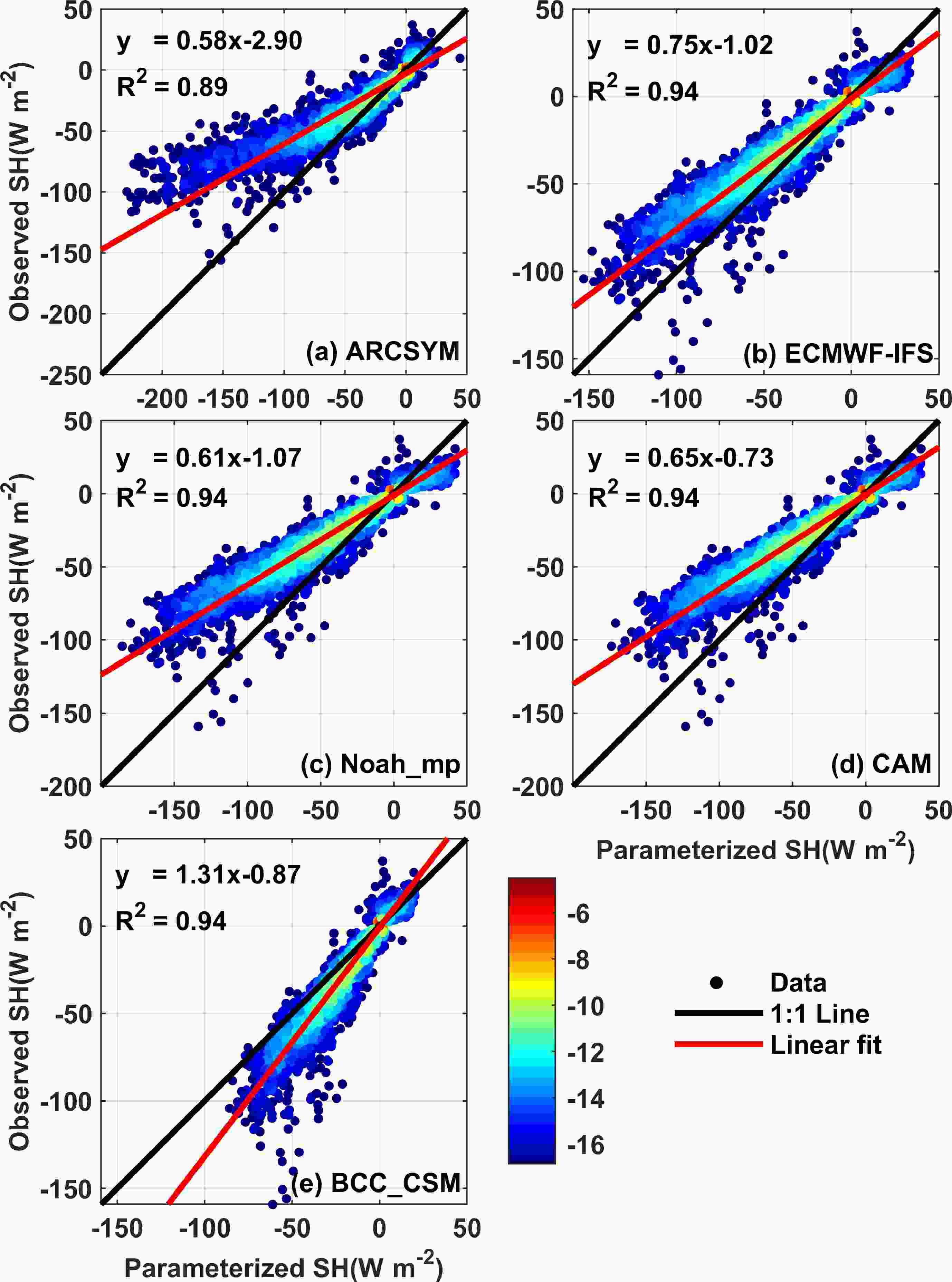
Figure 2. Same as in Fig.1, but for the sensible heat flux (SH).
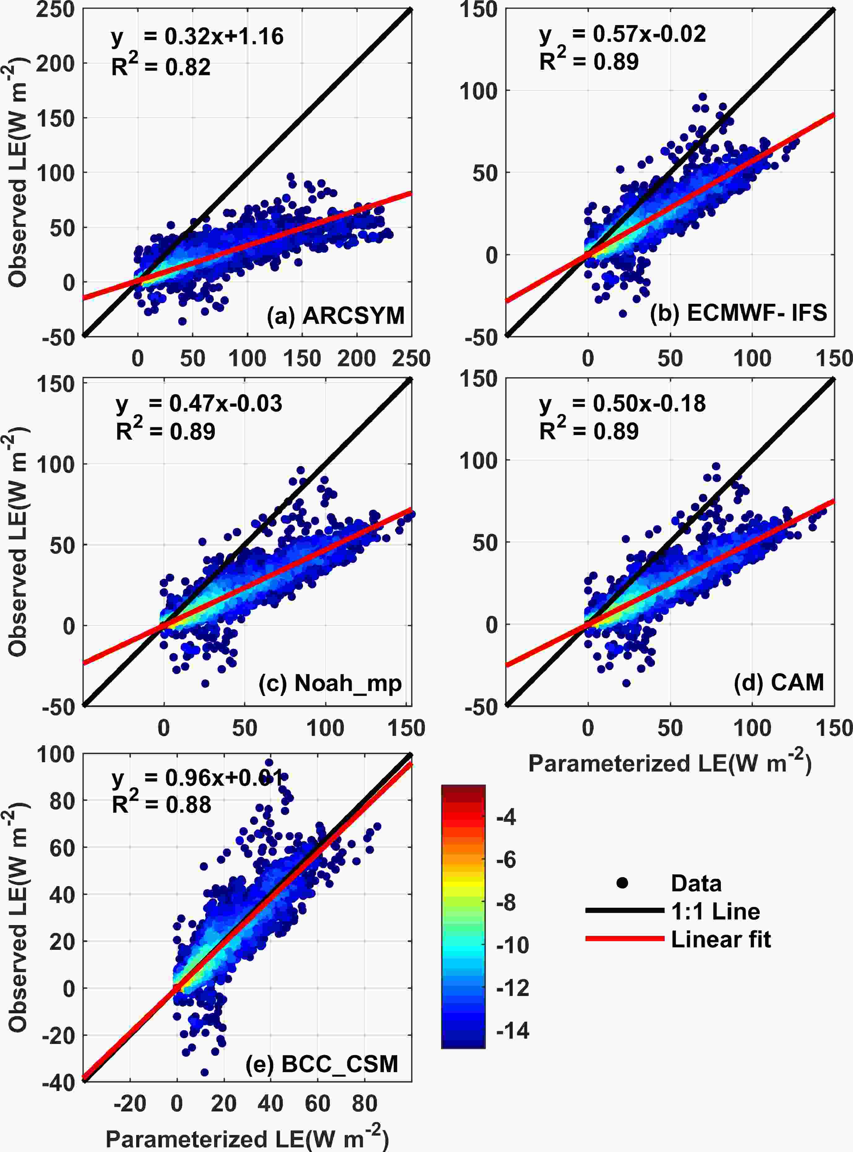
Figure 3. Same as in Fig.1, but for the latent heat flux (LE).
Table 3 gives the statistics of error analysis for five models. For τ, all models present the same correlation coefficient (CC) of 0.94, but Noah_mp produces the best error statistics with the smallest normalized root mean square error (RMSE) and mean bias (MB) and the optimal normalized standard deviation (σ). However, ARCSYM has the worst performance in error statistics for the τ, and the value of RMSE, σ, and MB is 2.92, 3.01, and 0.31, respectively. For the SH, although CAM presents a higher CC, the performance of CAM is not the best compared with other models in terms of RMSE and MB. On the contrary, the smallest MB of −7.93 is derived by ECMWF-IFS, and the smallest RMSE of 0.53 and the best σ of 0.75 are induced from BCC_CSM. For the LE, it is evident that BCC_CSM has a much smaller RMSE and MB than the other models, while ARCSYM performs the worst among the five models.
ARCSYM ECMWF-IFS Noah_mp CAM BCC_CSM τ CC 0.94 0.94 0.94 0.94 0.94 RMSE 2.92 0.41 0.33 0.35 0.79 σ 3.01 0.80 0.97 1.03 0.48 MB 0.31 −0.03 0.00 0.01 −0.08 SH CC 0.91 0.94 0.94 0.95 0.94 RMSE 1.12 0.62 1.03 0.92 0.53 σ 1.76 1.33 1.62 1.51 0.75 MB −13.16 −7.93 −16.00 −14.55 8.37 LE CC 0.87 0.92 0.92 0.92 0.91 RMSE 2.66 1.10 1.58 1.41 0.41 σ 2.90 1.61 1.95 1.81 0.95 MB 22.89 10.46 15.68 14.21 0.58
Notes: ${\text{CC} } = \dfrac{ { { {\rm{cov} } } (m,o)} }{ { {\sigma _m}{\sigma _o} } }, {\text{ RMSE} } = \sqrt {\dfrac{1}{N}\displaystyle\sum\limits_{i = 1}^N { { {({m_i} - {o_i})}^2} } } $, $ \sigma = \frac{ {\sqrt {\dfrac{1}{N}\displaystyle\sum\limits_{i = 1}^N { { {({m_i} - {\mu _m})}^2} } } } }{ {\sqrt {\dfrac{1}{N}\displaystyle\sum\limits_{i = 1}^N { { {({o_i} - {\mu _o})}^2} } } } } $, $ {\text{ MB} } = \dfrac{1}{N}\displaystyle\sum\limits_{i = 1}^N {({m_i} - {o_i})} ,$ where m refers to the simulation results, o indicates the observation results, and μ is the average value of a dataset. RMSE and σ are both normalized with the standard deviation of observation. Bold fonts indicate the best results.Table 3. The statistical characteristics for comparison between parameterization and observation.
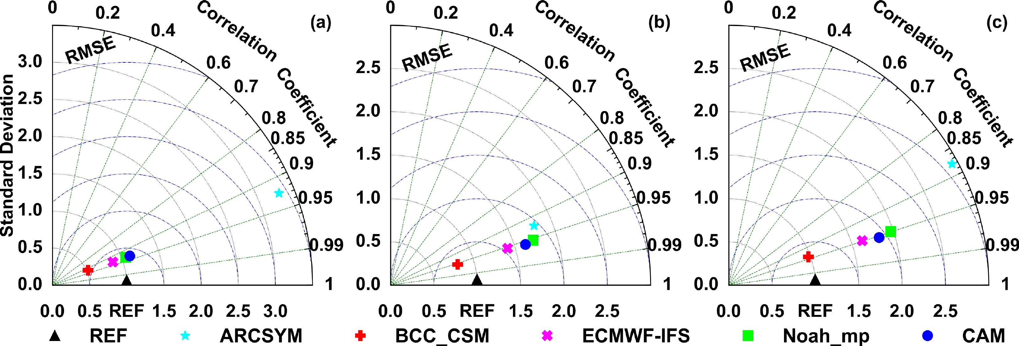
The Taylor diagram is often used to evaluate model performance comprehensively. As shown in Fig. 4a, the locations of simulated τ from CAM, Noah_mp, and ECMWF-IFS are all close to the reference point, while that from ARCSYM presents the farthest distance to the reference point. For the SH and LE, the locations of the five models in the Taylor diagram show a similar distribution pattern, i.e., the distances from the reference point from near to far are BCC_CSM, ECMWF-IFS, CAM, Noah_mp, and ARCSYM. Hence, we synthetically conclude that BCC_CSM performs best in simulating the turbulent fluxes over the Antarctic landfast sea-ice surface among the five models, although it produces a slightly inferior τ. In contrast, ARCSYM is the least applicable model for producing turbulent fluxes.
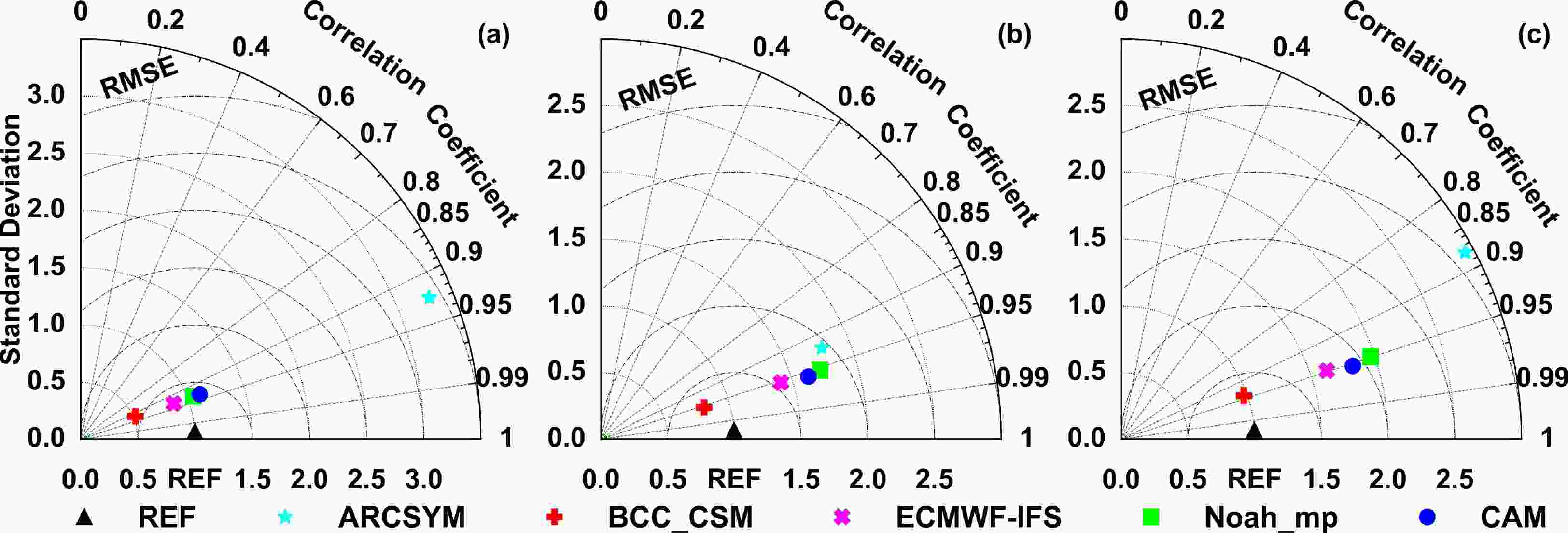
Figure 4. Taylor diagrams for the comparison between the parameterized and observed values of (a) τ, (b) SH, and (c) LE. REF refers to the observations.
Brunke et al. (2006) made an intercomparison of simulated turbulent fluxes from four numerical models, including ARCSYM and ECMWF-IFS, using the data collected over the Arctic sea-ice surface during the SHEBA field experiment. They also found that ARCSYM calculated a significantly overestimated τ, and ECMWF-IFS performed better than ARCSYM for modeling τ, SH, and LE. However, ARCSYM performs better in SHEBA than in our dataset due to a more reasonable parameter setting and applicability of ARCSYM in the Arctic. Interestingly, our results indicate a fairly good simulation of the LE by BCC_CSM compared with the performance of BCC_CSM in SHEBA (Lu et al., 2013). Overall, the models reproduce the turbulent momentum flux better than the turbulent heat fluxes in terms of RMSE and σ. To further clarify the causes for the differences in the performance of various models, we further investigate the behavior of stability functions and roughness lengths in numerical models in sections 3.2 and 3.3.
-
ARCSYM directly adopts Cm ~ Rib and Ch, Cq ~ (ΔT, U) relations to calculate turbulent fluxes instead of using the traditional bulk method; thus, it is not discussed in this section. Under unstable conditions, the other models all employ the Paulson1970 functions. However, the models use different stability functions under stable conditions (i.e., HDB88 functions for ECMWF-IFS, Z98 functions for BCC_CSM and CAM, and B71 functions for Noah_mp), which may influence their performance. Notably, the stability functions under stable conditions for wind speed, potential temperature, and specific humidity are the same in each model.
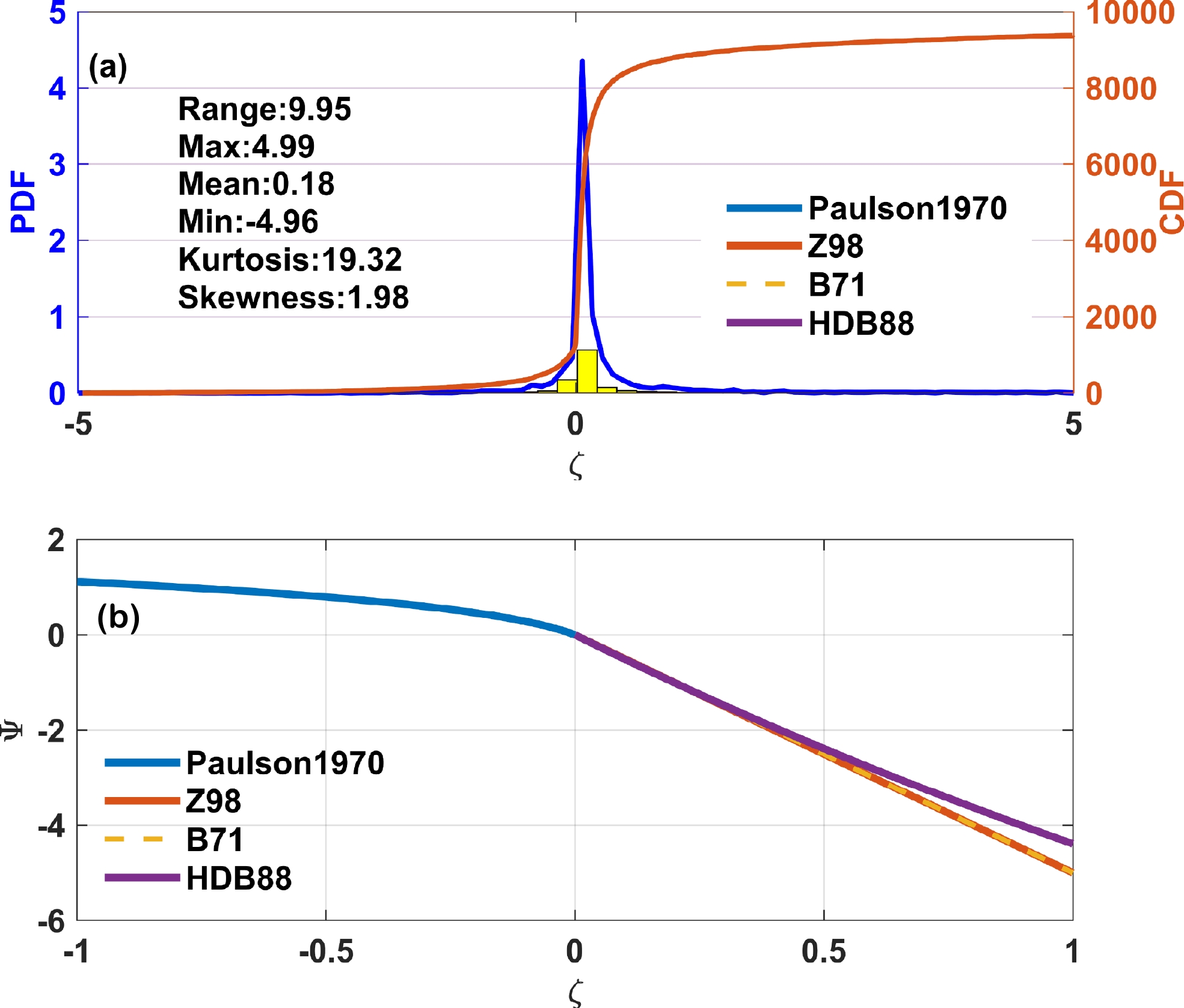
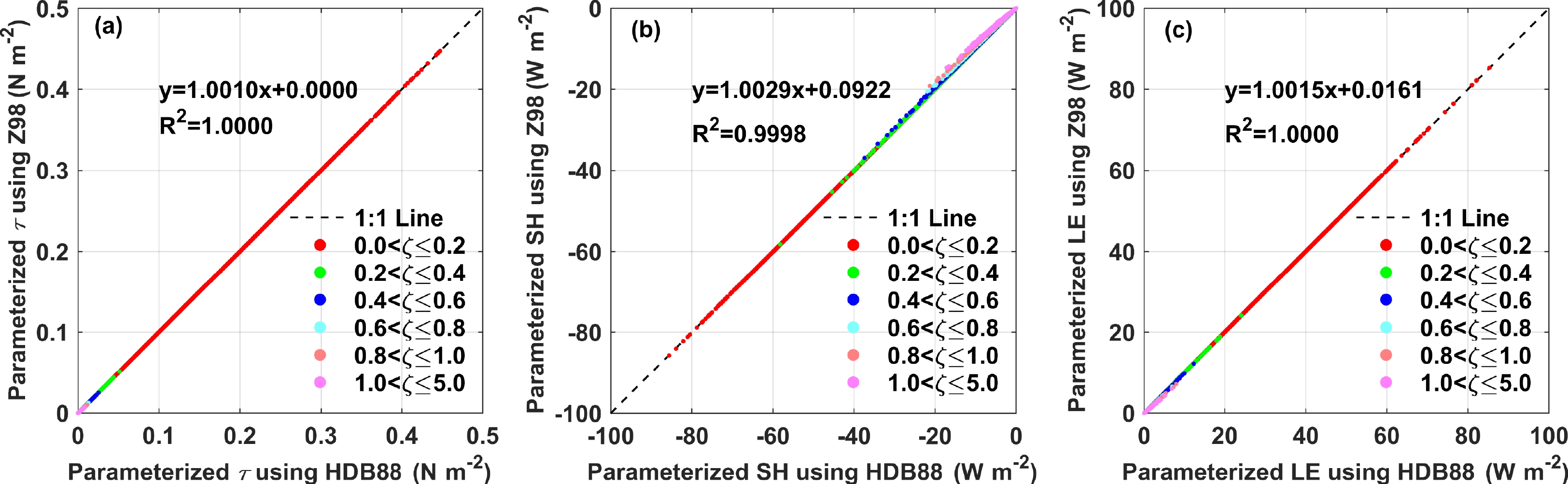
To quantify the impact of stability functions on model performance, we present the distribution of ζ during the observation period and deduce the difference in bulk turbulent exchange coefficients induced by different stability functions. As shown in Fig. 5a, the ζ lies between −1 and 1, accounting for 91.8% of the total sample; the following analysis focuses on this interval. The difference between B71 and Z98 functions is found to be negligible. Still, the HDB88 functions yield a larger value than the B71 and Z98 functions (Fig. 5b). The difference between the HDB88 functions and the other two functions tends to increase with the increase of ζ. When ζ = 1, the value of the HDB88 functions is −4.4, but it reaches −5 for B71 and Z98 functions. Figure 6 compares the parameterized turbulent fluxes using different stability functions under a stable condition with z0m = 10−3 m, z0t = 10−5 m, and z0q = 10−5 m, as suggested by Liu et al. (2020a). The results indicate that the differences in the parameterized turbulent fluxes caused by using different stability functions are negligible. However, the comparison of parameterized SH and LE by using different stability functions slightly deviates from the 1:1 line under strongly stable conditions (1 < ζ ≤ 5).
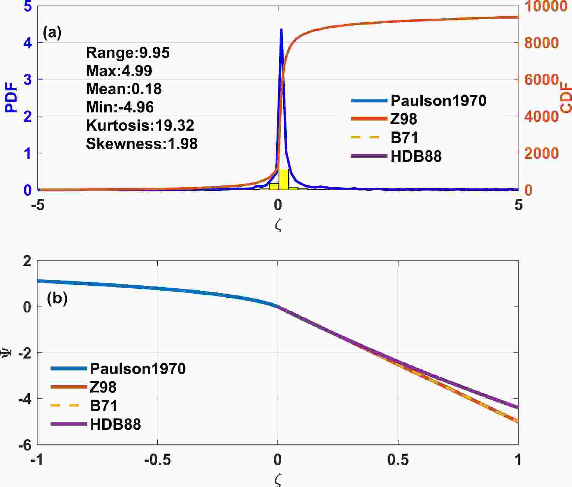
Figure 5. (a) The histograms, probability, and cumulative density functions of ζ and (b) the intercomparison of stability functions for both wind speed and potential temperature.
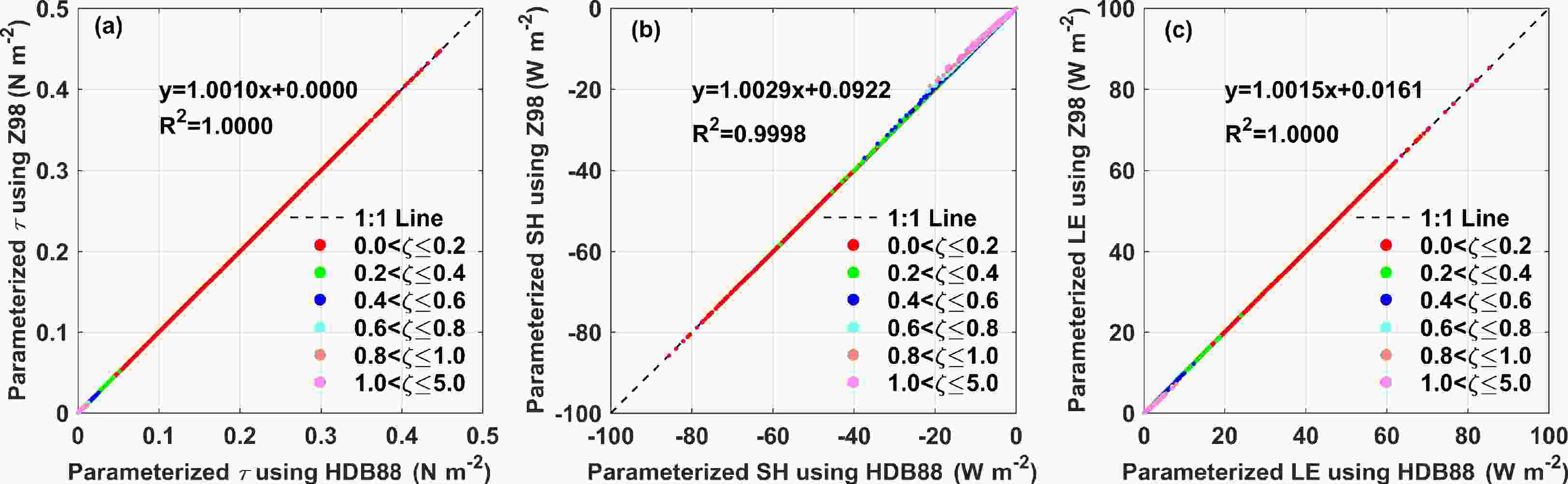
Figure 6. The comparison of parameterized (a) τ, (b) SH, and (c) LE by using different stability functions under stable conditions with z0m = 10−3 m and z0t (z0q) = 10−5 m. The dots with different colors correspond to different stability intervals.
In addition, we follow the theoretical method proposed by Andreas (2002) to assess the behavior of these stability functions. Four metrics, the gradient Richardson number (Ri), the Deacon numbers for wind speed (Dm) and for potential temperature (Dh), and the turbulent Prandtl number (Prt), are used to examine the behavior of stability functions. For each stability function, the four metrics in the limit of laminar flow are compared with the theoretical values (Table 4). As shown in Table 4, as ζ approaches infinity, the B71, HDB88, and Z98 functions produce the same Deacon numbers (i.e., Dm, Dh) and Prt, equivalent or close to the theoretical limits. However, the gradient Richardson numbers derived from B71, HDB88, and Z98 functions are 0.2, 1.43, and 1, respectively. Following Lu et al. (2013), the gradient Richardson number should equal 1 in a laminar flow. Therefore, we confer that the Z98 functions can represent stratification effects better under stable conditions.
Φm, Φh Dm Dh Ri Prt B71 0 0 0.20 1 HDB88 0 0 1.43 1 Z98 0 0 1 1 Laminar 0 0 ~1 ~0.71 Table 4. A comparison of the four models’ dimensionless stability functions in the limit of very stable stratification (ζ→∞).
-
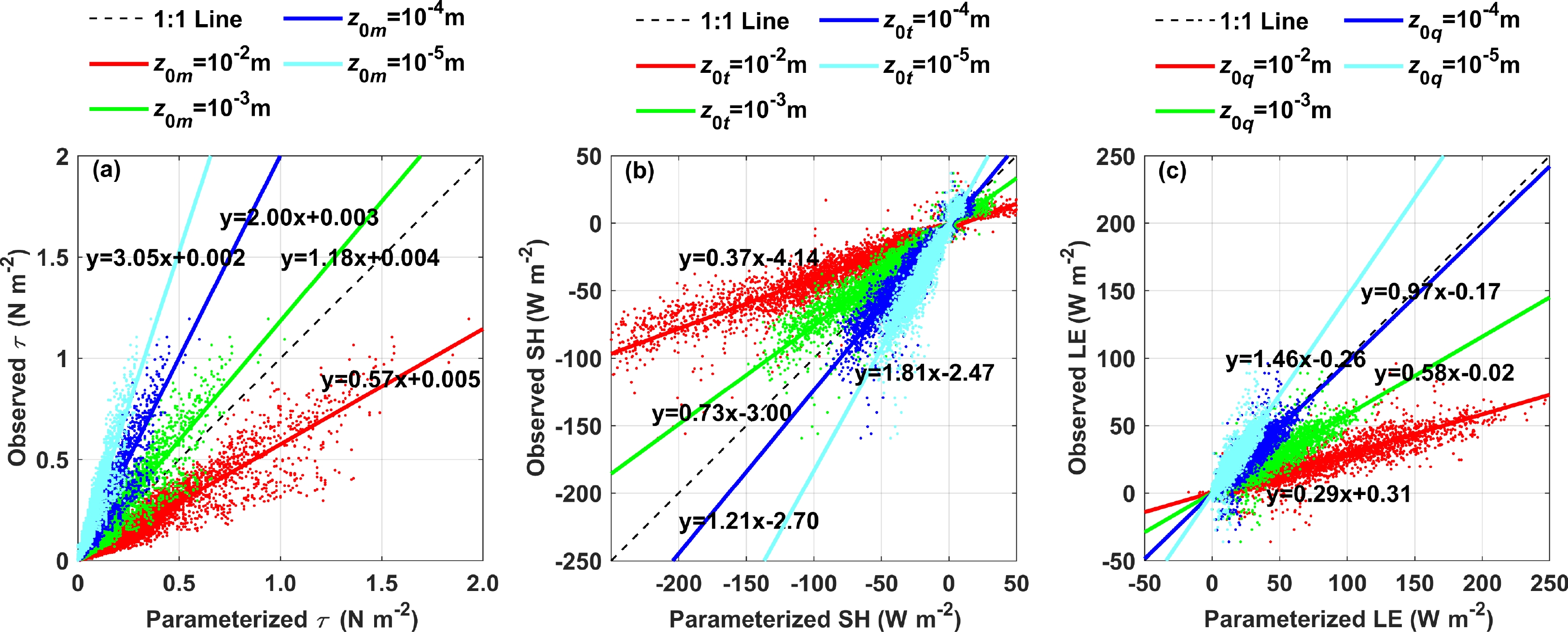
To examine the influence of roughness lengths on simulations, we make a set of sensitivity test experiments. In experiment I, we set the same stability functions (Z98 functions under stable conditions and Paulson1970 functions under unstable conditions) but various z0m from 10−2 to 10−5 m to examine the impact of z0m on the simulation of τ by solving Eqs. (1) and (4). Figure 7a shows that the simulated τ decreases sharply as the magnitude of z0m goes down. The τ simulated with z0m of 10−5 m is 18.7 % of that with z0m of 10−2 m. Meanwhile, the experiment gives a more appropriate magnitude of 10−3 m for z0m. The best reference constant of z0m is 1.9 × 10⁻³ m, and this is used in the next two experiments to examine the influence of z0t and z0q on the simulation of turbulent heat fluxes. To test the sensitivity of z0t on the simulated SH, we set z0t varying from 10−2 to 10−5 m (experiment II). Our result indicates that the simulated SH with z0t of 10−5 m is 20.4% of that with z0t of 10−2 m (Fig. 7b). The fitting line, with z0t equal to 10−4 m, is the closest one to 1:1 line. Experiment III examines the sensitivity of z0q in simulating the LE. As shown in Fig. 7c, the simulated LE when z0q is equal to 10−5 m is 19.9% of the simulated LE when z0q is equal to 10−2 m.
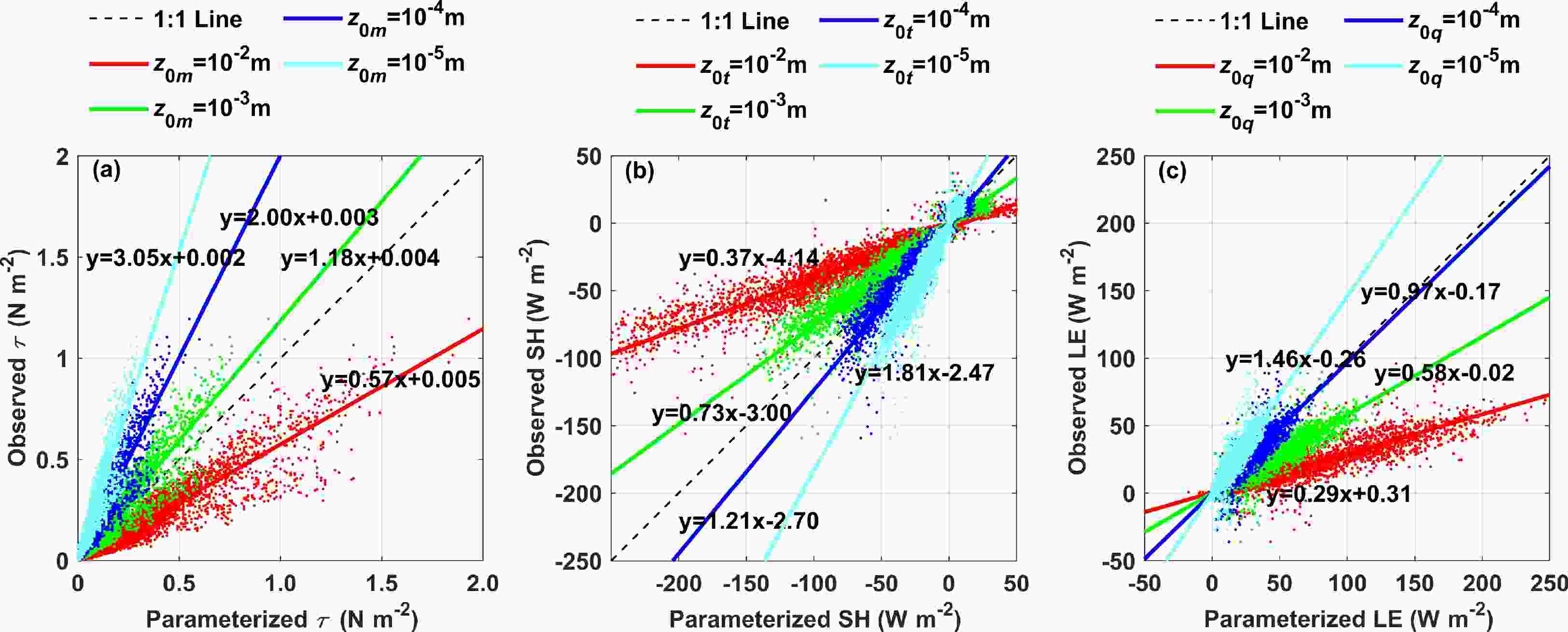
Figure 7. The sensitivity of z0m, z0t, and z0q on the simulation of (a) τ, (b) SH, and (c) LE, respectively. The different colors in subplots represent the comparison between simulated turbulent fluxes by different settings of roughness lengths and observed turbulent fluxes.
Hence, when roughness lengths change from 10−2 to 10−5 m, the τ is the most sensitive to the variation of z0m, while the SH shows the least sensitivity to the variation of z0t. On the other hand, the roughness lengths ranging from 10−2 to 10−5 m have been widely reported in different field experiments in Antarctica (King and Anderson, 1994; Cassano et al., 2001; Andreas et al., 2005; van den Broeke et al., 2005; Liu et al., 2020a), but different roughness length schemes within this range make a significant influence on the simulation of turbulent fluxes. Therefore, we can infer that the choice of roughness lengths is more critical to the simulation of turbulent fluxes than the settings of stability functions.
-
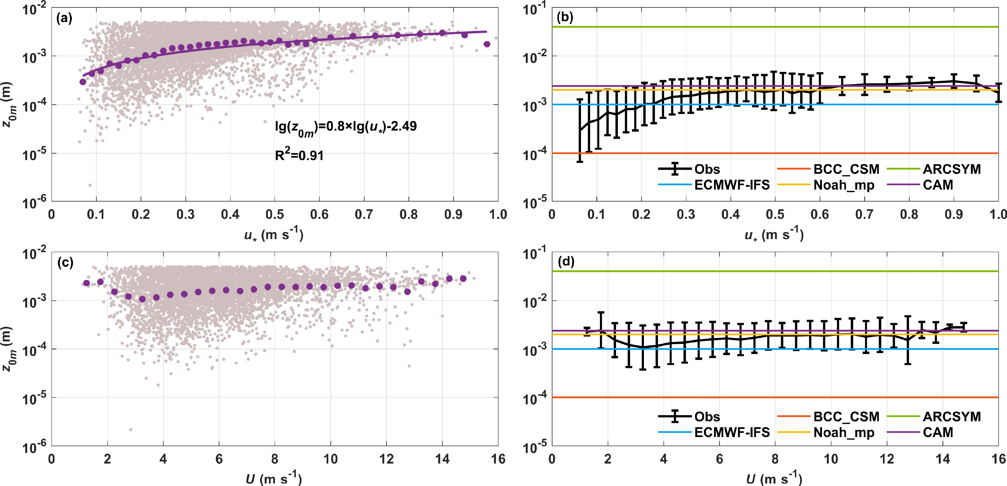
To reveal the characteristics of roughness lengths over the Antarctic landfast sea-ice surface and explain the performance in five numerical models, we apply the same quality control as Andreas et al. (2010) and calculate the observed values of z0m, z0t, and z0q according to Eqs. (1)–(6). Figure 8 presents the variation of z0m with wind speed and friction velocity. Figures 8a and 8b show that z0m continually increases in the range of u* ≤ 0.4 m s−1, while it reaches a constant of around 10−3 m when u* > 0.4 m s−1. The best-fit line of lg(z0m) = 0.8lg(u*)−2.49 can capture the variation of z0m with u*. Figures 8c and 8d show that z0m decreases, at first, with U increasing to 2.5 m s−1, and then shows a slight upward trend for U less than 6 m s−1, before finally fluctuating around a constant, about 10−3 m, for U larger than 6 m s−1. The asynchronous variation of z0m with u* and U under light wind or small u* conditions may result in the increase of Cm with the decrease of U even under near-neutral stratification, which has been observed by various field experiments (al-Jabburi, 2010; Grachev et al., 2011; Zhu and Furst, 2013; Mahrt et al., 2015; Patil et al., 2016). However, Cm should be independent of wind speed under near-neutral stratification in the MOST framework. Liu et al. (2020b) attributed this unexpected variation of Cm under near-neutral conditions in light winds to the non-local transport caused by large-scale eddies. Under moderate and large u* or U conditions, the variation of z0m is consistent with that over the Arctic sea-ice surface during the SHEBA experiment (Brunke et al., 2006). On the other hand, it can be found that, on average, z0m used in Noah_mp is the closest to the observed z0m, while the difference between z0m used in ARCSYM and the observed z0m is the largest. Hence, Noah_mp produces the most reliable simulated τ, but ARCSYM performs the worst.
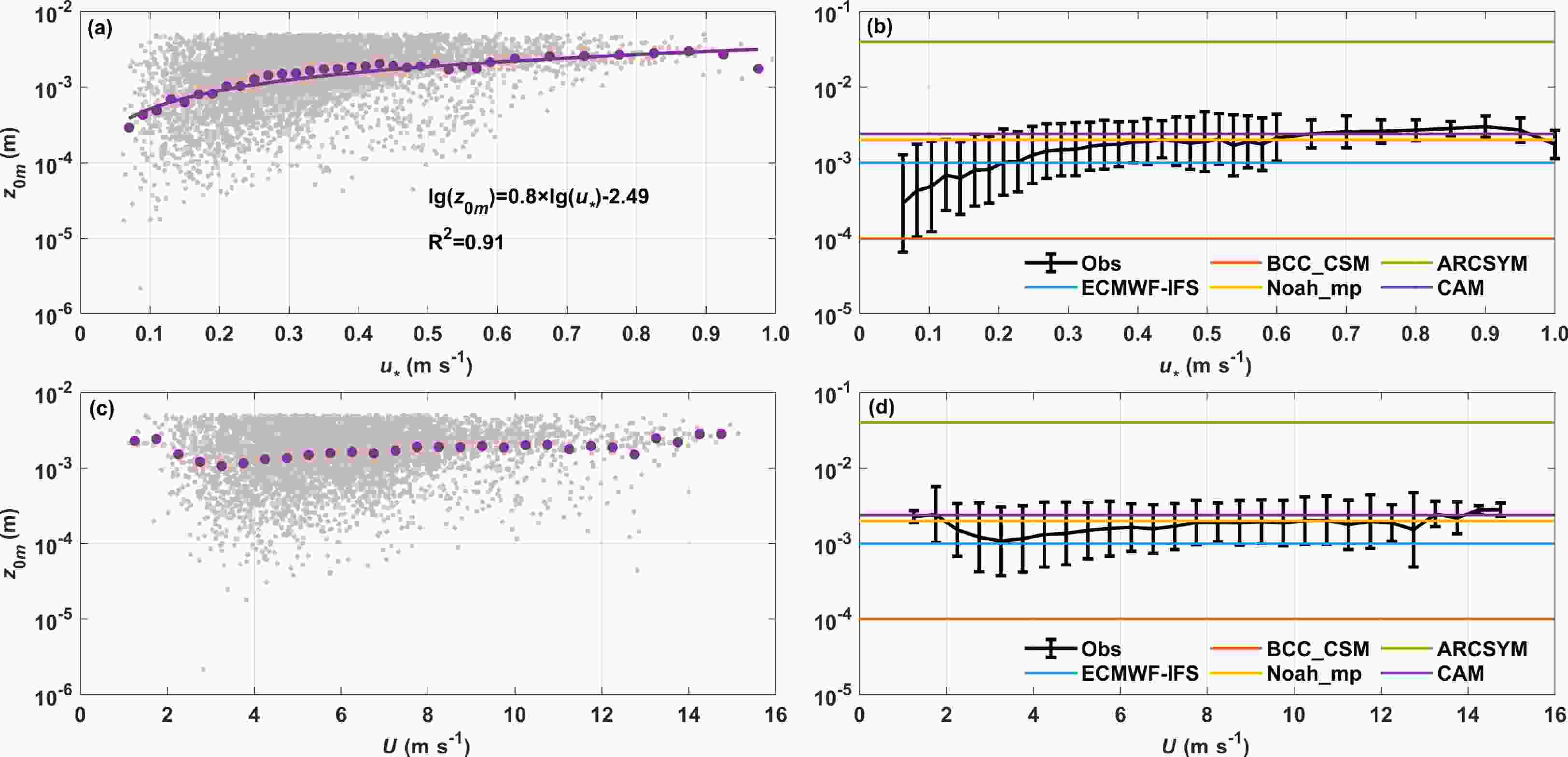
Figure 8. The calculated and bin-averaged value of z0m for (a, b) friction velocity u* and (c, d) wind speed U. The u* bins are 0.02 m s−1 wide when u* is less than 0.6 m s−1 and 0.05 m s−1 wide for larger u*; the U bins are 0.5 m s−1 wide; the error bars are ±1 standard deviation in the bin means. The values of z0m used in BCC_CSM, ARCSYM, ECMWF-IFS, Noah_mp, and CAM are also shown.
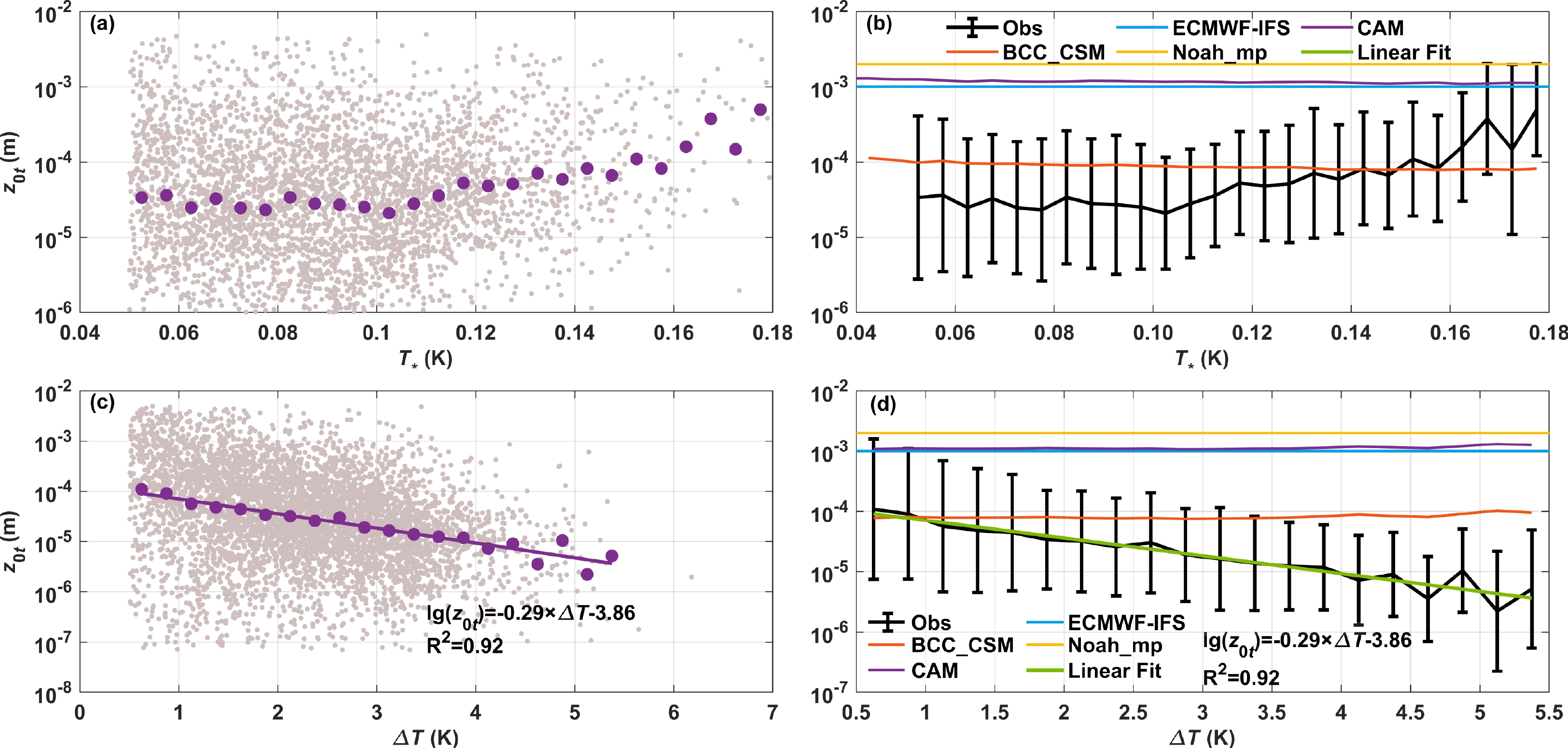
Figure 9 displays the variation of z0t with T* and ΔT. From Figs. 9a and 9b, it can be seen that z0t fluctuates around 5 × 10⁻⁵ m when T* ≤ 0.12 K and shows an increasing trend when T* ˃ 0.12 K. While Figs. 9c and 9d show that z0t decreases gradually with the increase of ΔT. Although the physical interpretation of the z0t is still under debate, some empirical or semi-empirical formulae have been proposed, which are typically related to z0m, R*, u*, or T* (Andreas, 1987; Zilitinkevich, 1995; Smeets and van den Broeke, 2008a, b; Yang et al., 2008). Here, we suggest a linear relationship of 1g(z0t) = −0.29ΔT−3.86, which provides a simple and available option to simulate the SH over the Antarctic landfast sea-ice surface. Comparing the settings of z0t in the models with the observed z0t, it is clear that only the z0t used in the BCC_CSM is within the standard deviation range of the observed z0t (Fig. 9b), while for other models, all selected z0t values are overestimated by 1–2 orders of magnitude. Both z0m and z0t affect the simulation of SH, as demonstrated in Eq. (5). Although the z0m of the BCC_CSM is underestimated by an order of magnitude, its z0t is overestimated by a factor of two, which results in a better performance in simulating SH. For the Noah_mp, CAM, and ECMWF-IFS, their z0m is close to the observed value, but their z0t is overestimated by 1–2 orders of magnitude, which lead to these models performing worse than BCC_CSM. Hence, the differences in z0m and z0t settings among the models can suitably explain their performance in simulating SH.
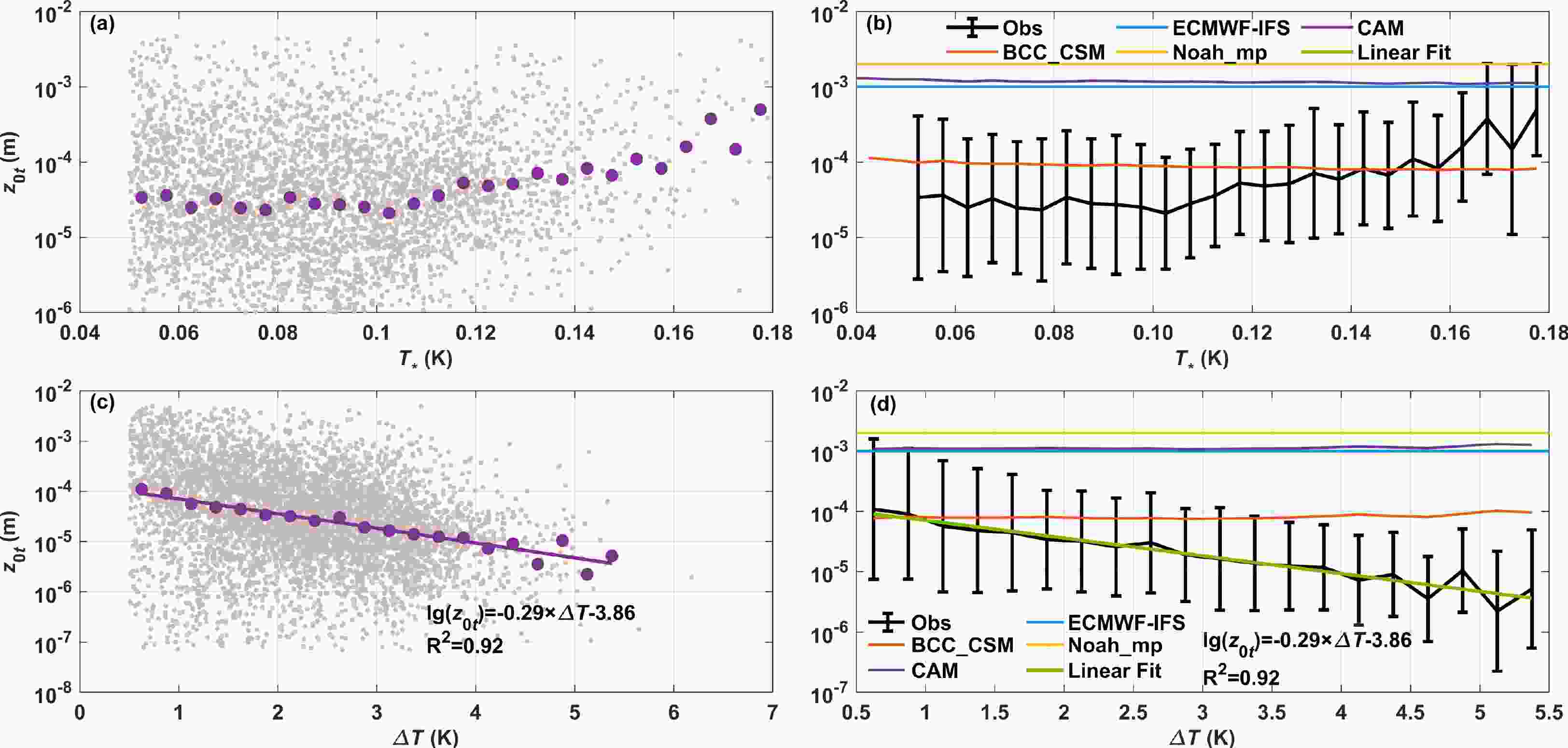
Figure 9. The calculated and bin-averaged value of z0t for (a, b) temperature scale T* and (c, d) temperature difference ΔT. The T* bins are 0.005 K wide and the ΔT bins are 0.25 K wide; the error bars are ±1 standard deviation in the bin means. The values of z0t used in BCC_CSM, ECMWF-IFS, Noah_mp, and CAM are also shown.
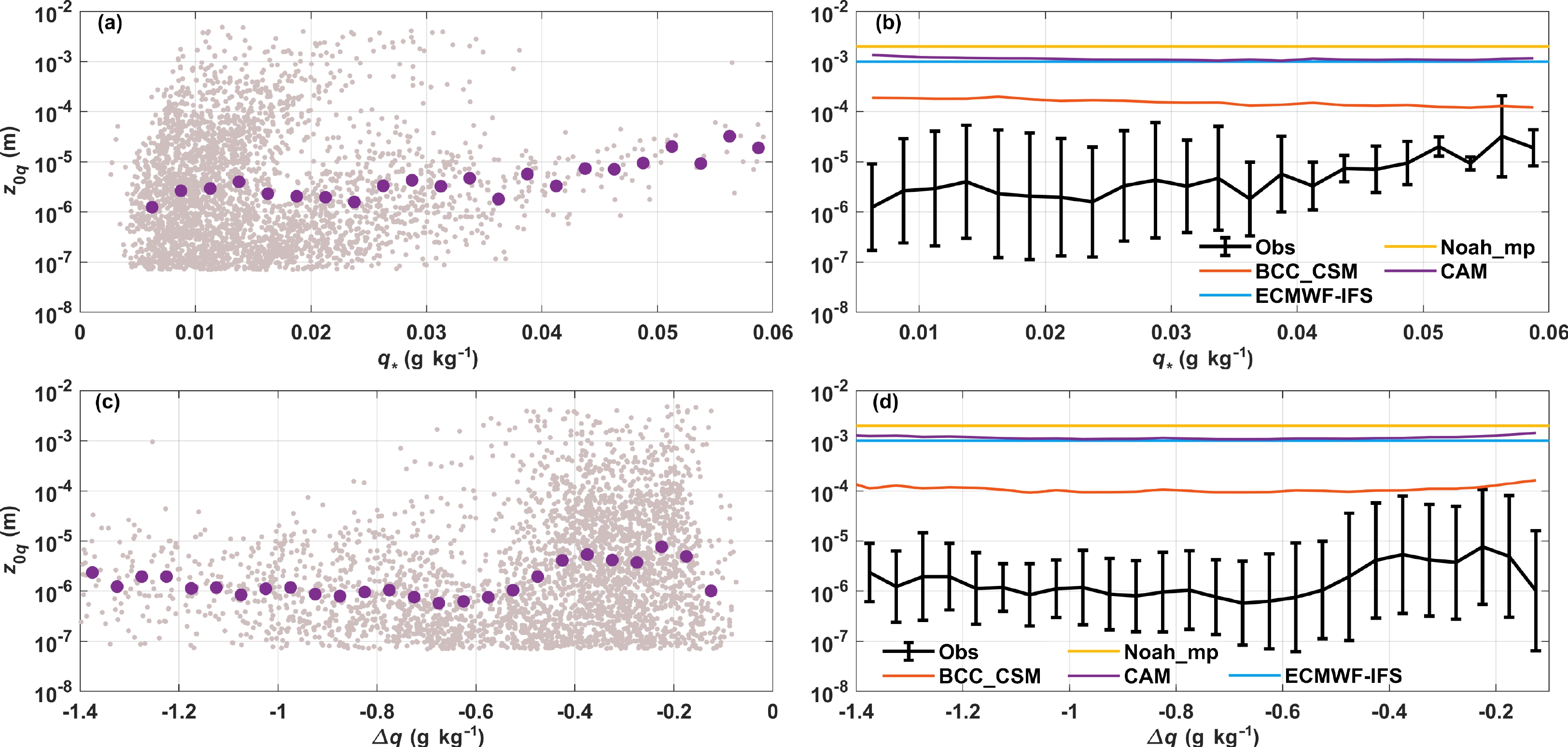
The z0q relations with specific humidity scale and specific humidity difference are shown in Fig. 10. In particular, Figs. 10a and 10b show that the bin-averaged z0q tends to be a constant at 3.2 × 10⁻⁶ m, but with relatively large standard deviations when q* ≤ 0.04 g kg−1, while z0q shows a slight increasing trend with the increase of q* in the region of q* ˃ 0.04 g kg−1, with sparse scatter in the data. In terms of humidity difference, z0q shows a subtle fluctuation around 10−6 m in the small Δq region (i.e., Δq ≤ −0.6 g kg−1), but it increases significantly when Δq ˃ −0.6 g kg−1. The mean z0q is 10−6 (3.5 × 10⁻⁶) m when Δq ≤ −0.6 g kg−1 (Δq ˃ −0.6 g kg−1). In addition, Figs. 10b and 10d show that the z0q used in BCC_CSM is approximately 1.5 orders of magnitude higher than observation, while the other models overestimate z0q even more drastically by up to 2.5 orders of magnitude. Interestingly, the overestimation in z0q seems to offset the underestimation in z0m, producing the best simulation of LE in BCC_CSM (Fig. 3e).
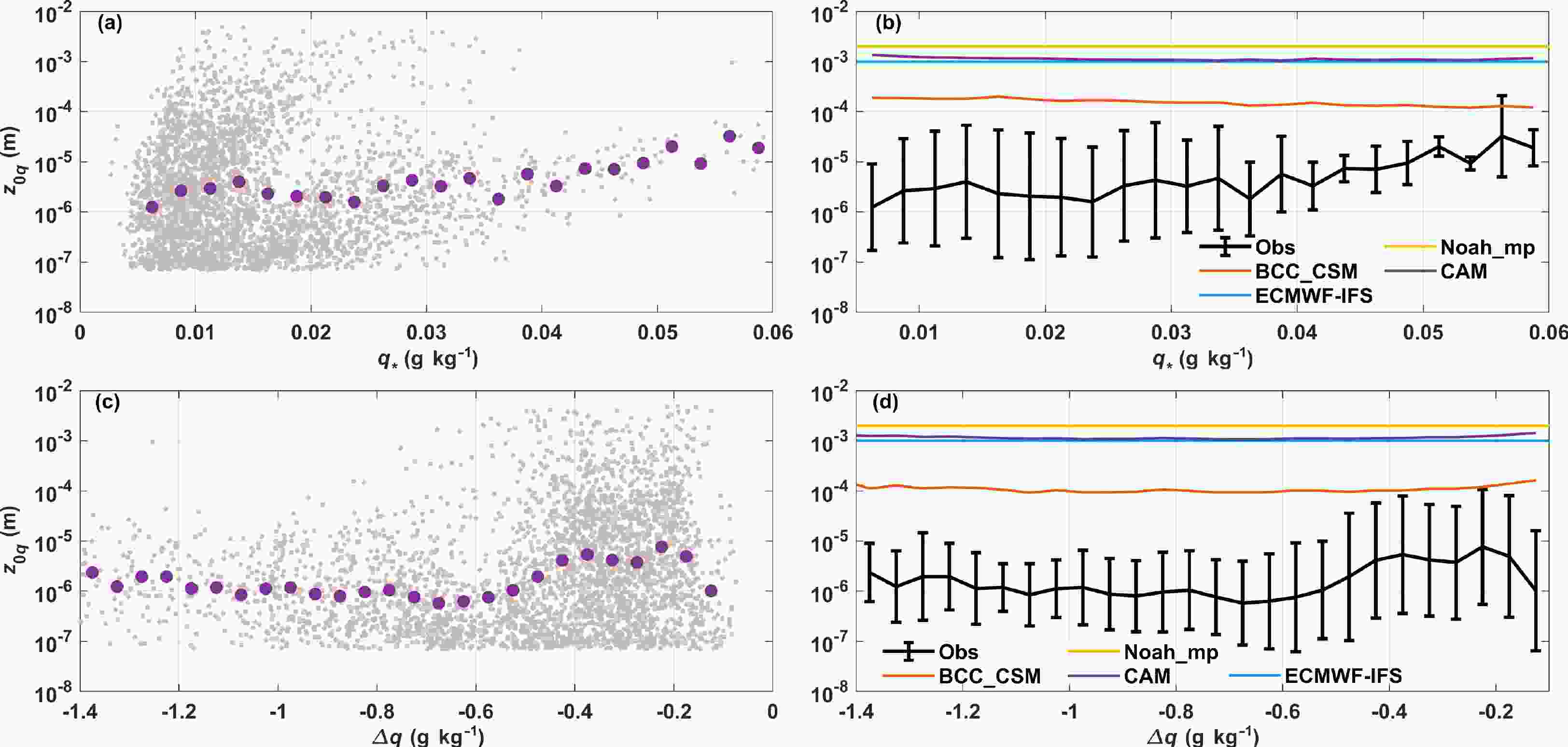
Figure 10. The calculated and bin-averaged value of z0q for (a, b) specific humidity scale q* and (c, d) specific humidity difference Δq. The width of the q* and Δq bins are 0.0025 g kg−1 and 0.05 g kg−1, respectively, and the error bars are ±1 standard deviation in the bin means. The values of z0q used in BCC_CSM, ECMWF-IFS, Noah_mp, and CAM are also shown.
To sum up, an integrated roughness length scheme is suggested according to the above results: (1) lg(z0m) = 0.8lg(u*)−2.49; (2) 1g(z0t) = −0.29ΔT−3.86; (3) z0q = 10−6 m (Δq ≤ −0.6 g kg−1) and z0q = 3.5 × 10⁻⁶ m (Δq ˃ −0.6 g kg−1). Figure 11 compares the turbulent fluxes from observation with the turbulent fluxes parameterized by employing the suggested stability functions (i.e., the Z98 functions) and the proposed integrated roughness lengths scheme. It can be found that the simulation results are in good agreement with the observations. The RMSE for τ, SH, and LE is 0.33, 0.33, and 0.41, respectively. In addition, the performance of the new parameterization scheme is better than that of the original parameterization scheme of any model.
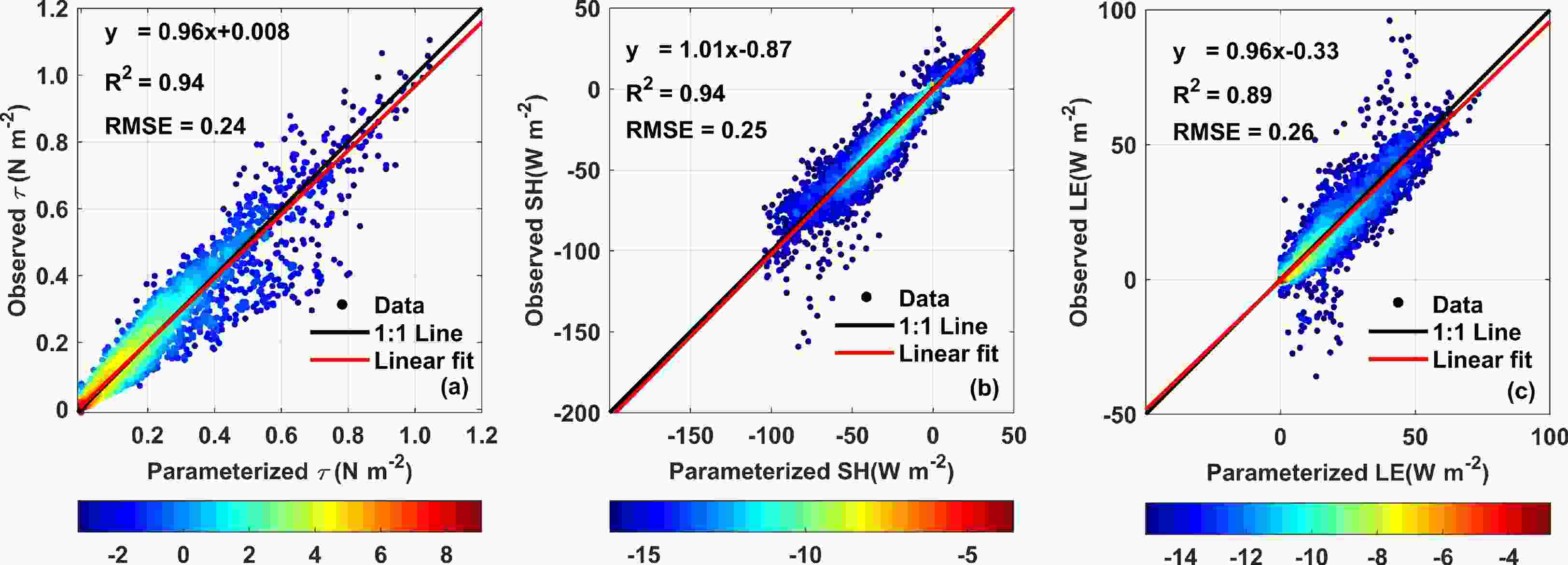
Figure 11. The comparison of the observed turbulent fluxes with the parameterized turbulent fluxes obtained by adopting the suggested roughness length scheme.
-
As described in section 2.3, the ECMWF-IFS, Noah_mp, CAM, and BCC_CSM models all use the common theoretical framework of MOST to parameterize turbulent fluxes. However, the applicability of the MOST under stable conditions is disputed. In very stable conditions, the MOST may not be applicable due to weak, intermittent, sporadic, patchy, and non-stationary turbulence (Sorbjan, 2006; Grachev et al., 2007; Sharan and Kumar, 2011). These characteristics of turbulence under stable stratification are related to various factors, e.g., gravity waves (Sun et al., 2004), density currents (Chenge and Brutsaert, 2005), low-level jets (Wei et al., 2018), and isopycnic slope flows (Chenge and Brutsaert, 2005). Grachev et al. (2013) suggested a primary threshold of flux Richardson number less than 0.2–0.25 for the applicability of MOST, based on spectral analysis. With further increases in stability, the classic MOST does not work, and the Richardson-Kolmogorov cascade dies out. Focusing on these issues, some efforts have been made to extend stability functions (Gryanik et al., 2020). However, the problem of establishing universal and robust stability functions for stable conditions remains to this day (Gryanik and Lüpkes, 2022).
On the other hand, as shown in Figs. 8–10, the calculated roughness lengths present large discrete situations, especially for z0t and z0q. Such uncertainties in the calculated roughness lengths can also be found in previous research over various surface types (Sun, 1999; Andreas, 2002; Yang et al., 2008; Andreas et al., 2010; Sicart et al., 2014; Liu et al., 2019). The considerable uncertainty may be attributed to insufficient knowledge regarding the physical mechanisms of surface roughness lengths (Hu et al., 2020). The observation results show that roughness lengths are influenced by many factors, e.g., surface geometric characteristics, friction velocity, molecular viscosity, surface temperature, humidity deficit, and surface moisture (Rigden et al., 2018). However, even the most popular roughness length scheme for the snow and ice surface proposed by Andreas (1987) cannot explain the large uncertainties of calculated roughness lengths. Further in-depth research on the mechanism of surface roughness lengths is necessary but still challenging due to insufficient measurements.
Notably, different averaging intervals used in the EC fluxes calculation procedures may affect the results. The choice of averaging time is determined by turbulent conditions. The averaging interval should not be too long or too short. If the interval is too long, non-turbulent contributions may be included, while using too short of an interval results in missed contributions from lower frequencies (Burba, 2013). The existence of an energy gap between synoptic and turbulent scales makes it possible to divide the flow into synoptic and turbulent parts by averaging over a specific time interval (approximately 30 minutes to 1 hour) (Stull, 1988). Therefore, the mandatory approach, among the most widely used ways to choose an averaging time, simply uses standard averaging times of 30 min or 1 hour (Foken et al., 2012). In glaciated areas, although some previous studies seem inclined to adopt a shorter period of 10 min (King, 1990; Cassano et al., 2001) or 15 min (Stössel et al., 2010), Guo et al. (2011) suggested an adequate averaging period of 30 minutes because low-frequency turbulence was very limited in contributing to the flux. In addition, the 30-min averaging time was also used in polar regions by other studies (Guest and Davidson, 1991; Vignon et al., 2017; Walden et al., 2017). Hence, we also chose 30 min as a reasonable averaging interval in this study.
Based on the data collected over the Antarctic landfast sea-ice surface from 8 April 2016 through 26 November 2016, this paper evaluates the parameterization schemes for turbulent fluxes in the selected five numerical models, including ARCSYM, ECMWF-IFS, Noah_mp, CAM, and BCC_CSM.
The statistics of error analysis indicate that Noah_mp reproduces the τ best, while BCC_CSM performs better than the other models in simulating the SH and LE. The simulation of turbulent surface fluxes is more sensitive to the choice of roughness lengths rather than the settings of stability functions, and the differences in the settings of roughness lengths among the models can well explain their performance in simulating turbulent fluxes. Notably, although BCC_CSM produces a near-flawless performance in simulating LE, the z0m used in BCC_CSM is underestimated by nearly a few orders of magnitude, and z0q is overestimated by about 1.5 orders of magnitude. Liu et al. (2020a) suggested a constant z0m of 1.9 × 10⁻³ m and a constant z0t of 3.7 × 10⁻⁵ m but did not calculate z0q. In this study, we suggest a constant z0q of 2.4 × 10⁻⁶ m for reference.
Additionally, this study investigates the variation of roughness lengths with corresponding scale parameters and the gradient of meteorological elements. Our results reveal that z0m continually increases with the increase of u* when u* ≤ 0.4 m s−1, while it tends to be a constant of around 10−3 m when u* > 0.4 m s−1; the variation of z0t with ΔT presents a linear relationship of 1g(z0t) = −0.29ΔT−3.86; and a noticeable difference of z0q is found between the region of Δq ≤ −0.6 g kg−1 (z0q = 10−6 m) and Δq ˃ −0.6 g kg−1 (z0q = 3.5×10⁻⁶ m). These results can help us set more appropriate roughness lengths in the models and enhance the parameterization schemes for turbulent fluxes over the Antarctic landfast sea-ice surface.
This study is based on a single in-situ observation, so the representativeness of our conclusions may be limited. The observation site in this study is also within a katabatic wind zone of the East Antarctic coast. It remains questionable whether our results still hold in other regions without katabatic wind, like the interior plateau of Antarctica. We need more in-situ observations in the Antarctic continent to answer this question.
Acknowledgements. We thank the Chinese Arctic and Antarctic Administration and Polar Research Institute of China for logistic support. This study is supported by the National Key Research and Development Program of China (Grant No. 2022YFE0106300), the National Natural Science Foundation of China (Grant Nos. 42105072, 41941009, 41922044), the Guangdong Basic and Applied Basic Research Foundation (Grant Nos. 2021A1515012209, 2020B1515020025), the China Postdoctoral Science Foundation (Grant Nos. 2021M693585), and the Norges Forskningsråd (Grant No. 328886).
| Instrument | Measurement quantities | Sampling rate | Installation height |
| SI-111 | Surface temperature (Ts) | 0.1 Hz | 1 m |
| HMP155 | Air temperature (Ta); Relative humidity (RH) | 0.1 Hz | 2 m |
| CS106 | Atmospheric pressure (Pa) | 0.1 Hz | 0.5 m |
| IRGASON | Three-dimensional velocity (Ux, Uy, Uz); Sonic temperature (θv); H2O Density ($\rho_{{\rm{H}}_2{\rm{O}}} $); Air Density (ρ) | 10 Hz | 2 m |
 AAS Website
 AAS WeChat