Increasing Surface UV Radiation in the Tropics and Northern Mid-Latitudes due to Ozone Depletion after 2010

It is well known that solar ultraviolet (UV) radiation is a major cause of skin cancer and damages the immune system and DNA in humans (Lucas et al., 2019). It also profoundly impacts agricultural productivity, terrestrial and aquatic ecosystems, and air quality (Douglass and Fioletov, 2011; Williamson et al., 2014). The importance of UV radiation in influencing global ecosystems has been widely discussed, noting that stratospheric ozone is a key factor in modulating the changes of UV radiation at the Earth’s surface. Stratospheric ozone levels began to decline in the late 1970s (Farman et al., 1985), which was mainly related to human use of chlorine- and bromine-containing compounds such as chlorofluorocarbons (CFCs) (Molina and Rowland, 1974; Solomon et al., 1986). This decrease in stratospheric ozone led to an increase in surface UV radiation via the creation of a hole in the ozone layer over the Antarctic (Gurney, 1998; Hegglin and Shepherd, 2009; Tourpali et al., 2009; Bais et al., 2015; Eleftheratos et al., 2020). After the Antarctic ozone hole was detected in the 1980s (Farman et al., 1985; Solomon, 1999), the signing and adherence to the Montreal Protocol (MP) in 1987 successfully reduced emissions of ozone-depleting substances. Following the MP, the stratospheric loading of chlorine/bromine peaked in the late 1990s and has since decreased, meaning that the stratospheric ozone levels were projected to recover, and the related increase in UV radiation at Earth’s surface should have been abated.

Many studies, however, have reported that while upper-stratospheric ozone started recovering from 1995 to 2016 following the MP, ozone concentrations in the lower stratosphere continue to show a declining trend (Kyrölä et al., 2013; Sofieva et al., 2017; Steinbrecht et al., 2017; Ball et al., 2018, 2019; Bourassa et al., 2018; Petropavlovskikh et al., 2019; Orbe et al., 2020; Dietmüller et al., 2021; Bognar et al., 2022), most likely because of the continued production and release of one particular type of CFC, trichlorofluoromethane (Montzka et al., 2018), or its dynamic transport caused by natural variability (Chipperfield et al., 2018; Dhomse et al., 2018; Morgenstern et al., 2018; Wargan et al., 2018). The Long-term Ozone Trends and Uncertainties in the Stratosphere (LOTUS) report (SPARC/IO3C/GAW, 2019) further pointed out that, between January 2000 and December 2016, statistically significant positive ozone trends were obtained throughout the upper stratosphere based on satellite and ground-based data; whereas, non-significant, negative ozone trends were consistently detected by multiple satellite sources in the post-2000 period for the middle and lower stratosphere over the tropics and Northern Hemisphere (NH) mid-latitudes. Due to this inconsistency between the changes in ozone in the upper and lower stratosphere after the 1990s, the recovery of the total ozone column (TCO) is not significant. In addition, there are other challenges to the alleged robustness of ozone recovery (Chipperfield, 2009; Ravishankara et al., 2009; Daniel et al., 2010; Wang et al., 2014; Xie et al., 2014; Tian et al., 2017; Zhang et al., 2018; Lu et al., 2019; He et al., 2022; Hu et al., 2022; Solomon et al., 2022; Zhang et al., 2023; Xia et al., 2023). Here, we find that the TCO in the tropics and Northern Hemisphere mid-latitudes started to significantly deplete again in the May-September period after around 2010, resulting in increased surface UV radiation.

The UV data (including cloud effects) in this study are from the Ozone Monitoring Instrument (OMI) and Tropospheric Emission Monitoring Internet Service (TEMIS) datasets; the ozone data are from the Multi-Sensor Reanalysis 2 (MSR-2), the Stratospheric Water and OzOne Satellite Homogenized (SWOOSH) and Microwave Limb Sounder (MLS) datasets; and the ClO, BrO, and HNO₃ data are from the MLS dataset. The OMI dataset (Hovila et al., 2013) with a horizontal resolution of 1° × 1° is used. In the TEMIS dataset (Van Geffen et al., 2017), the UV index and UV dose data of version 2.2 are given on a 0.25° × 0.25° lat./lon. grid covering the whole globe. For MSR-2 (Van Der A et al., 2015), the monthly mean total column ozone spans 1979–2020 with a horizontal resolution of 0.5° × 0.5°. The SWOOSH dataset (Davis et al., 2016) with a 2.5° zonal mean value is used. The MLS (Livesey et al., 2015), version 5, measures daily atmospheric chemical species with global coverage from 82°N to 82°S and a vertical resolution of ~3 km.

The TOMCAT/SLIMCAT three-dimensional offline chemical transport model (Chipperfield, 2006; Feng et al., 2021) is used to investigate the processes of ozone-related chemistry. The model uses horizontal temperature and wind from the European Centre for Medium-Range Weather Forecasts (Hersbach et al., 2020) (ERA5). This study ran a historical reproduction experiment with a horizontal resolution of about 2.8° × 2.8° with 32 vertical levels from the surface to 65 km. The model provides a good representation of stratospheric chemistry compared with observations (Chipperfield, 2006; Feng et al., 2011).

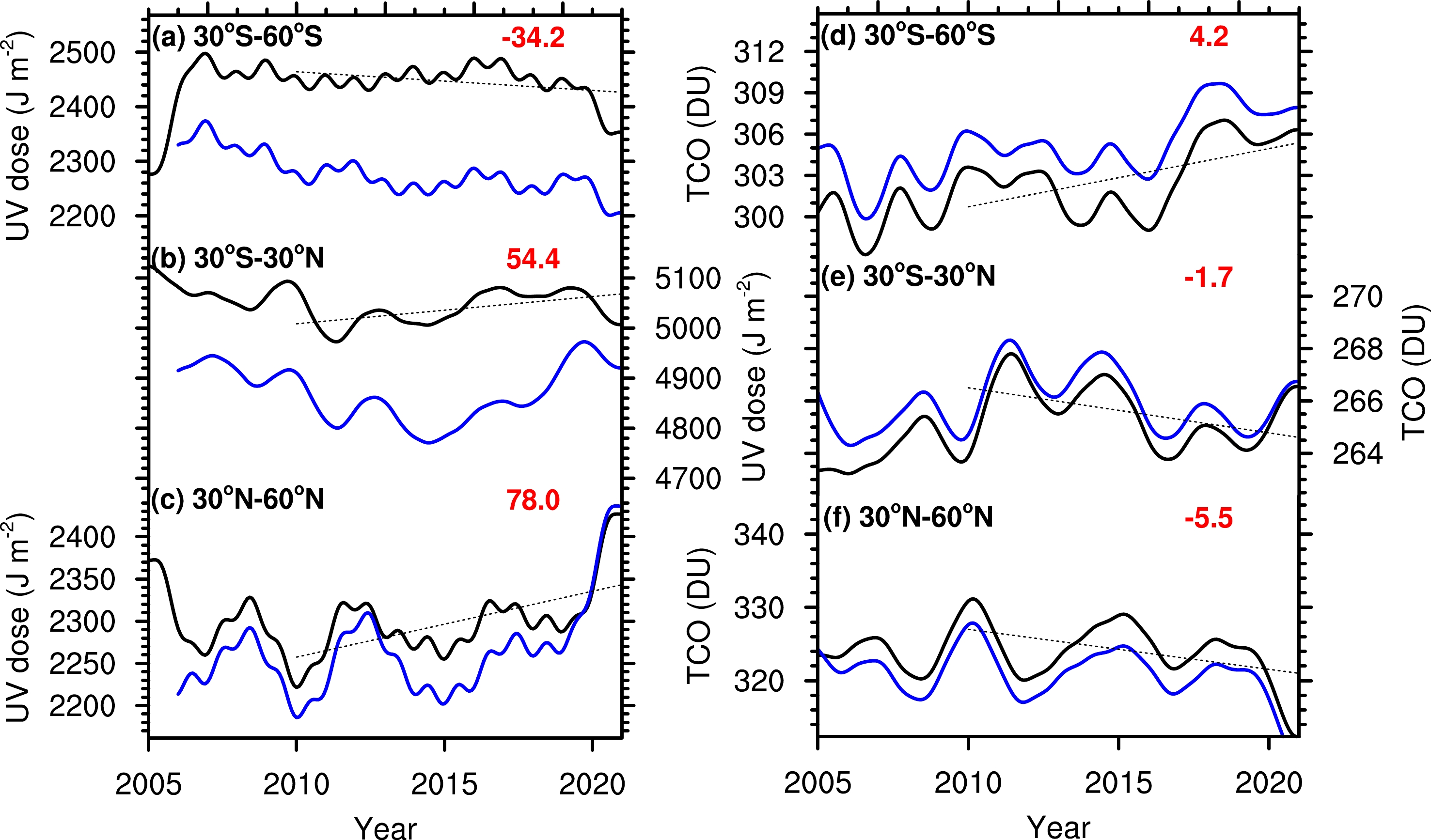
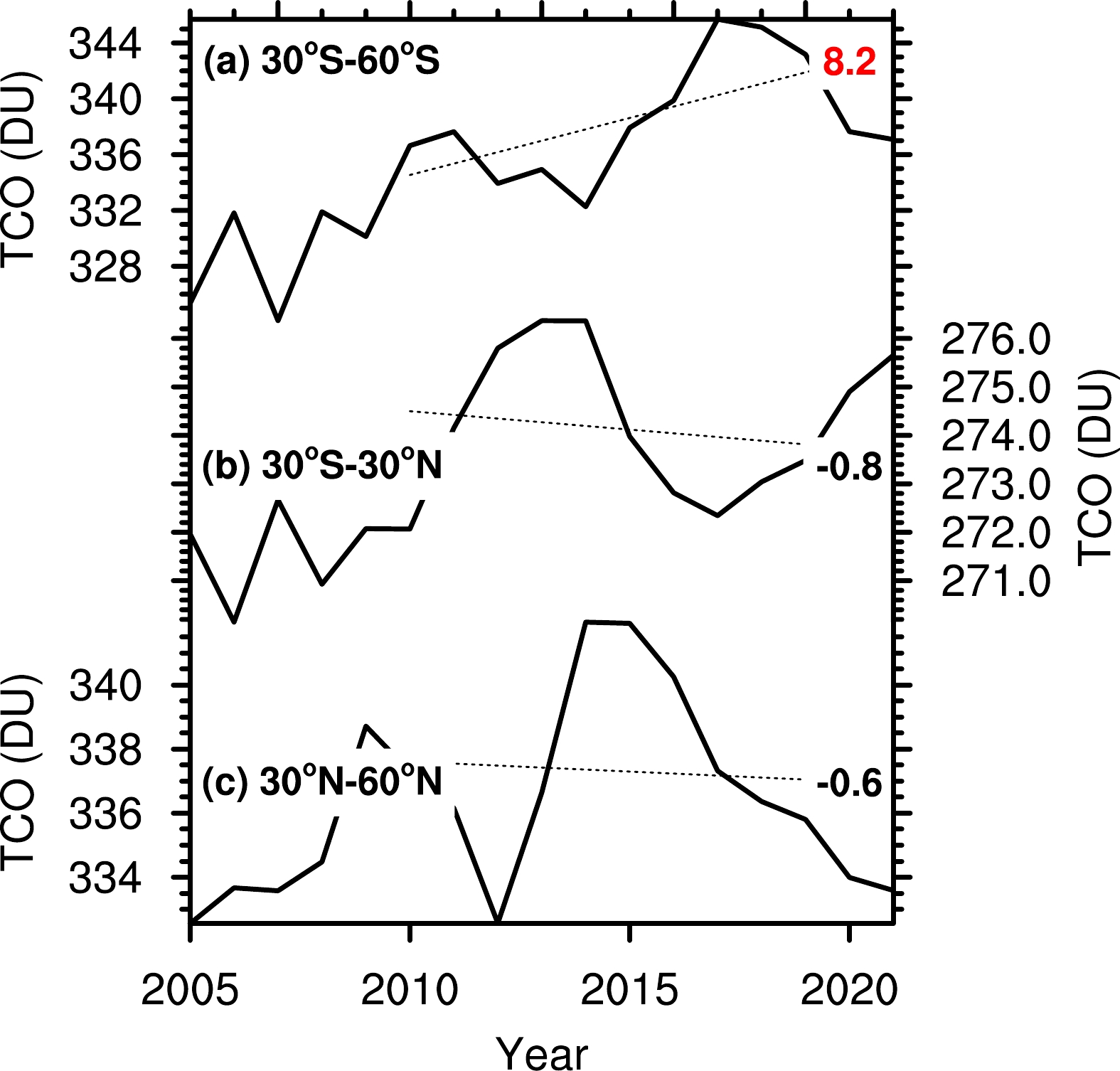
Figures 1a–c show the UV changes at the surface level from 2005 to 2020 at different latitudes obtained from the Ozone Monitoring Instrument (OMI) and Tropospheric Emission Monitoring Internet Service (TEMIS) data. For a description of the data, please refer to the previous section. Due to the sparse population at the poles, we focus only on the UV changes between 60°S and 60°N. We find that surface UV shows increasing trends over the tropics and NH mid-latitudes (Figs. 1b, c) but a decreasing trend over Southern Hemisphere (SH) mid-latitudes (Fig. 1a) from around 2010 onwards. The linear trends are −34.2 ± 14.7 J m^–2 (10 yr)^–1, 54.4 ± 14.3 J m^–2 (10 yr)^–1, and 78.0 ± 17.3 J m^–2 (10 yr)^–1 over the SH mid-latitudes (Fig. 1a), tropics (Fig. 1b) and NH mid-latitudes (Fig. 1c), respectively, for the period 2010–20 (all significant at the 2σ level using a Student’s t-test). The results from the two datasets show a high degree of consistency.

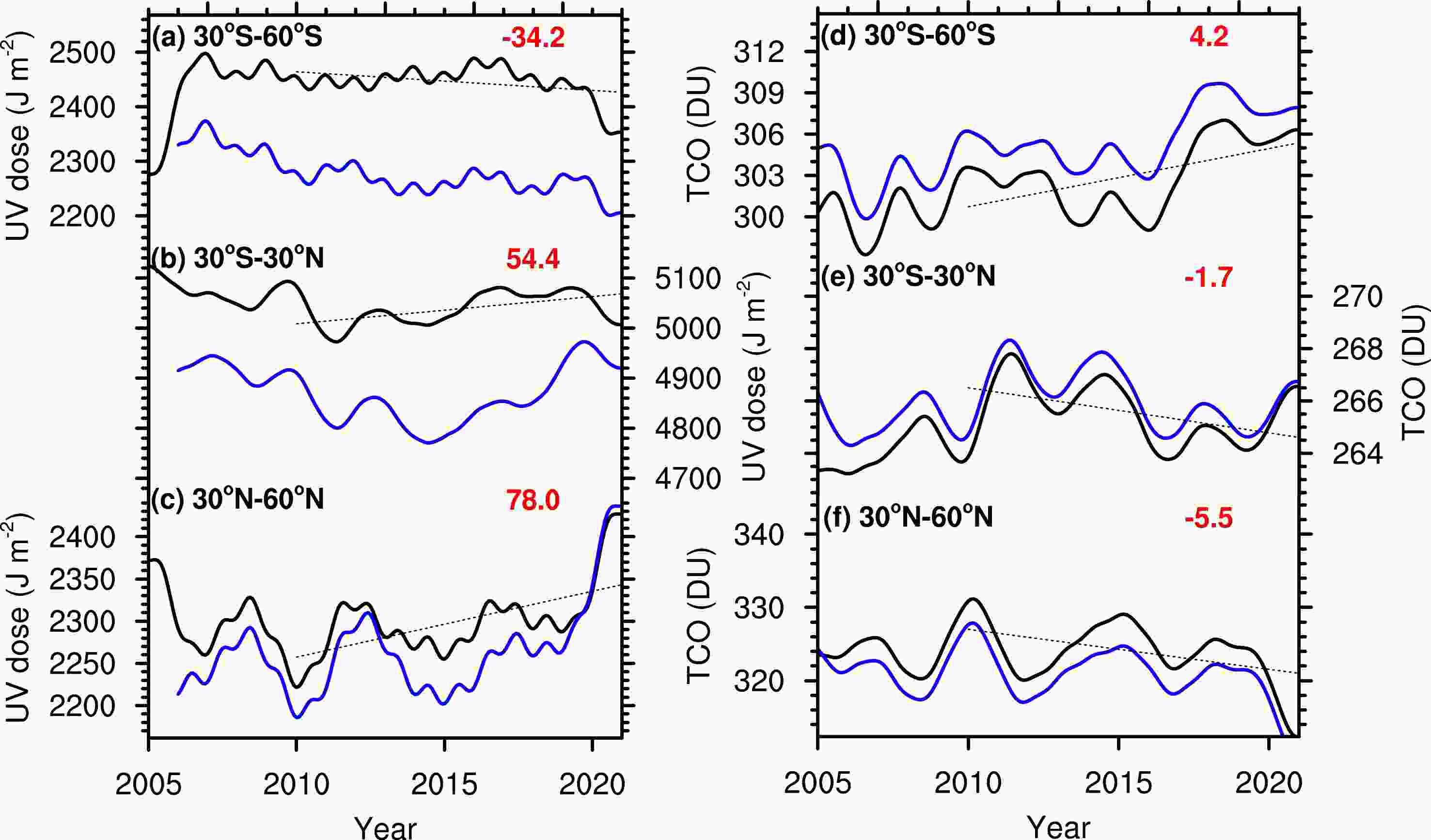
Figure 1.  The UV and TCO changes between different latitudinal belts from 2005 to 2020. The (a–c) UV and (d–f) TCO changes between (a, d) 60°S and 30°S, (b, e) between 30°S and 30°N, and (c, f) between 30°N and 60°N. UV is based on OMI (black line) and TEMIS (blue line) data; TCO is based on MSR-2 (black line) and SWOOSH (blue line) data. For data information, please refer to section 2. Linear trends (black straight dotted lines) are calculated by linear regression. The number close to the right-y-axis is the linear trend value for 2010–2020 based on the OMI dataset for UV and the MSR-2 dataset for TCO. The red and black values indicate statistical significance and non-significance, respectively, at the 2σ level using the Student’s t-test. The unit for the UV trend is J m^–2 (10 yr)^–1, and for the TCO trend, it is DU (10 yr)^–1. Low-pass filtering (to filter out periods <3 years) was performed on the UV and TCO changes before calculating the trend.

TCO is one of the main drivers of changes in surface UV. Figures 1d–f show the changes in TCO from 2005 to 2020 at latitudes between 60°S and 60°N obtained from the Multi-Sensor Reanalysis 2 (MSR-2) and The Stratospheric Water and OzOne Satellite Homogenized (SWOOSH) data (see Methods). From around 2010 onward, the UV trends are in close agreement with those of TCO. That is, the linear trends of ozone are 4.2 ± 1.1 DU (10 yr)^–1 (Fig. 1d), −1.7 ± 0.5 DU (10 yr)^–1 (Fig. 1e), and −5.5 ± 1.9 DU (10 yr)^–1 (Fig. 1f) in the SH mid-latitudes, tropics and NH mid-latitudes, respectively, for the period 2010–20 (significant at the 2σ level using a Student’s t-test). The correlation coefficients between the TCO and UV variations over this period are −0.51, −0.95, and −0.88 in the SH mid-latitudes, tropics, and NH mid-latitudes, respectively, demonstrating that the changes in TCO played a key role in the changes of UV during this period. It should be noted that, aside from ozone, factors such as cloud cover, aerosols, air pollutants, and surface reflectance also affect UV (Kylling et al., 2000; Bernhard et al., 2007; den Outer et al., 2010; Douglass and Fioletov, 2011). The positive trend of TCO in the SH mid-latitudes (Weber et al., 2022) (Fig. 1d) may be related to decreasing the emissions of ozone depletion substances, resulting in the negative trend of UV (Fig. 1a). Next, we focus on investigating the significant decreasing TCO trends over the tropics and NH mid-latitudes (Figs. 1e, f), which are responsible for the increasing UV trends (Figs. 1b, c).

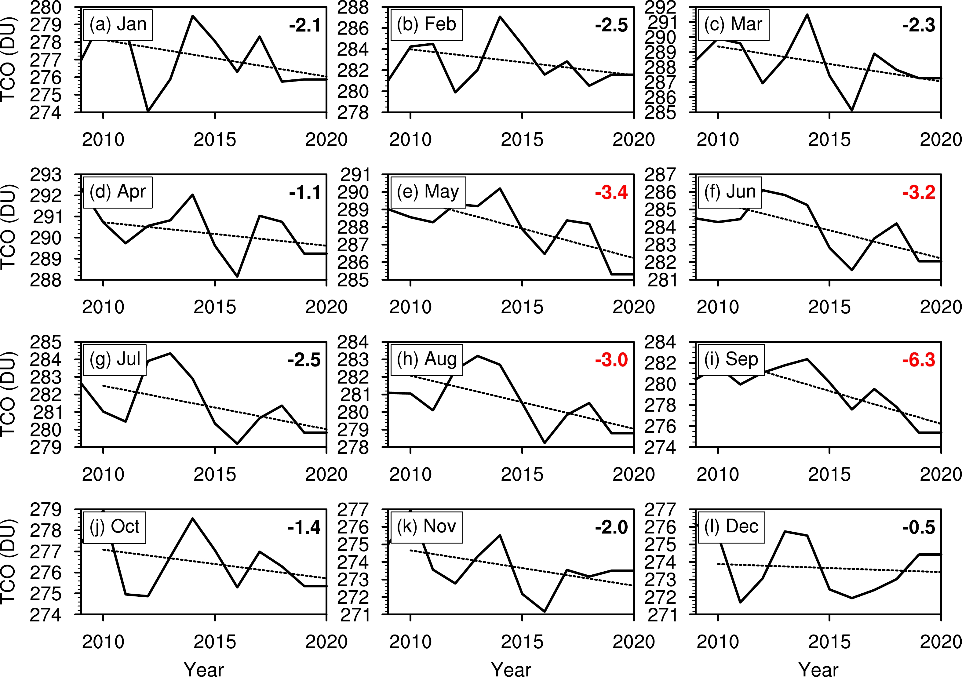
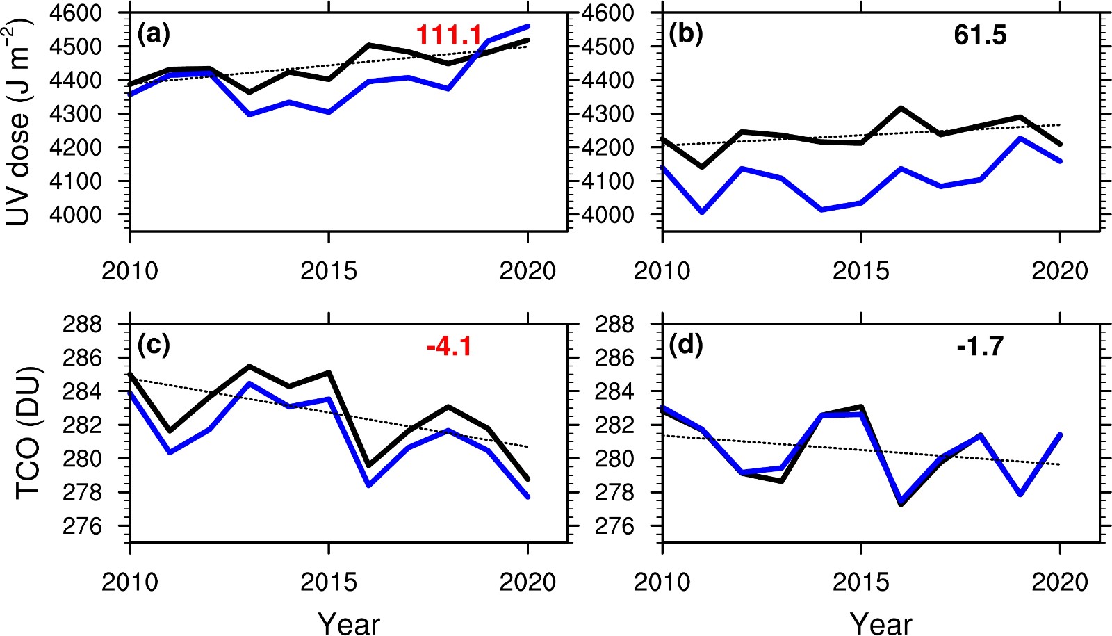
Figure 2 presents the TCO changes in the tropics and NH mid-latitudes for each month from 2010 to 2020. The linear decreasing TCO trends are strong and significant, mainly from May–September. Figure 3 shows the UV and TCO changes in the 30°S–60°N latitudinal belt from 2010–20, averaged from May–September and October– April. The positive UV trend for the May–September average is statistically significant at the 2σ level (Fig. 3a) and much larger than that for the October–April average (Fig. 3b). This is because ozone depletion over 30°S–60°N for the May–September average is strong and statistically significant at the 2σ level (Fig. 3c), but it is much weaker for the October–April average (Fig. 3d). Note that the correlation coefficient between TCO and UV variations for the May–September average is −0.94, which further supports the premise that the changes in TCO led to the changes of surface UV during this period.

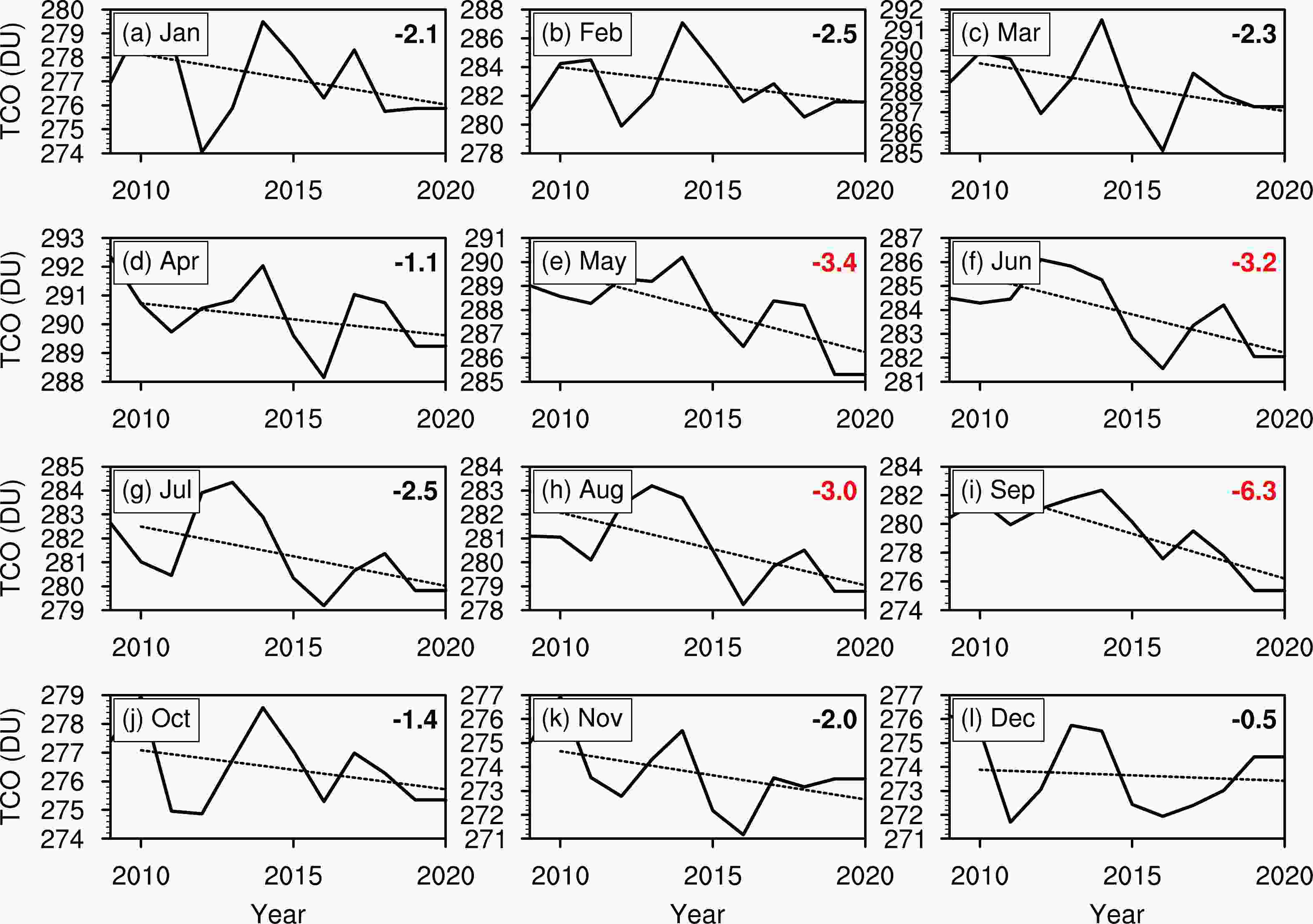
Figure 2.  TCO trends in the 30°S–60°N latitudinal belt from 2010 to 2020 for 12 months. The TCO is based on the MSR-2 dataset. For data information, please refer to section 2. The linear trends (black straight dotted lines) were calculated by linear regression. The number close to the right-hand y-axis is the linear trend value [units: J m^–2 (10 yr)^–1] for 2010–20. Red and black values denote statistical significance and non-significance, respectively, at the 2σ level using a Student’s t-test. A three-point running average was performed on the TCO changes for 12 months before calculating the trend.

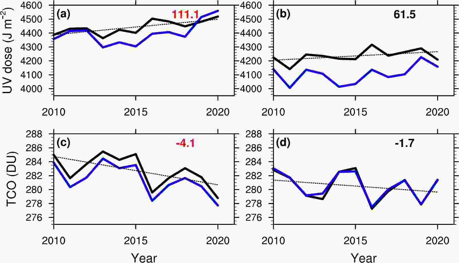
Figure 3.  The (a, b) UV and (c, d) TCO changes in the 30°S–60°N latitudinal belt from 2010 to 2020 for the (c, d) May–September average and the (b, d) October–April average. UV is based on (black line) OMI and (blue line) TEMIS data; TCO is based on (black line) MSR-2 and (blue line) SWOOSH data. For data information, please refer to section 2. Linear trends (black straight dotted lines) are calculated by linear regression. The number close to the right-hand-y-axis is the linear trend value for 2010–20 based on the OMI dataset for UV and based on the MSR-2 dataset for TCO. Red and black values denote statistical significance and non-significance, respectively, at the 2σ level, using a Student’s t-test. The unit for the UV trend is J m^–2 (10 yr)^–1, and for the TCO trend, it is DU (10 yr)^–1. A three-point running average was performed on the UV and TCO changes before calculating the trend.

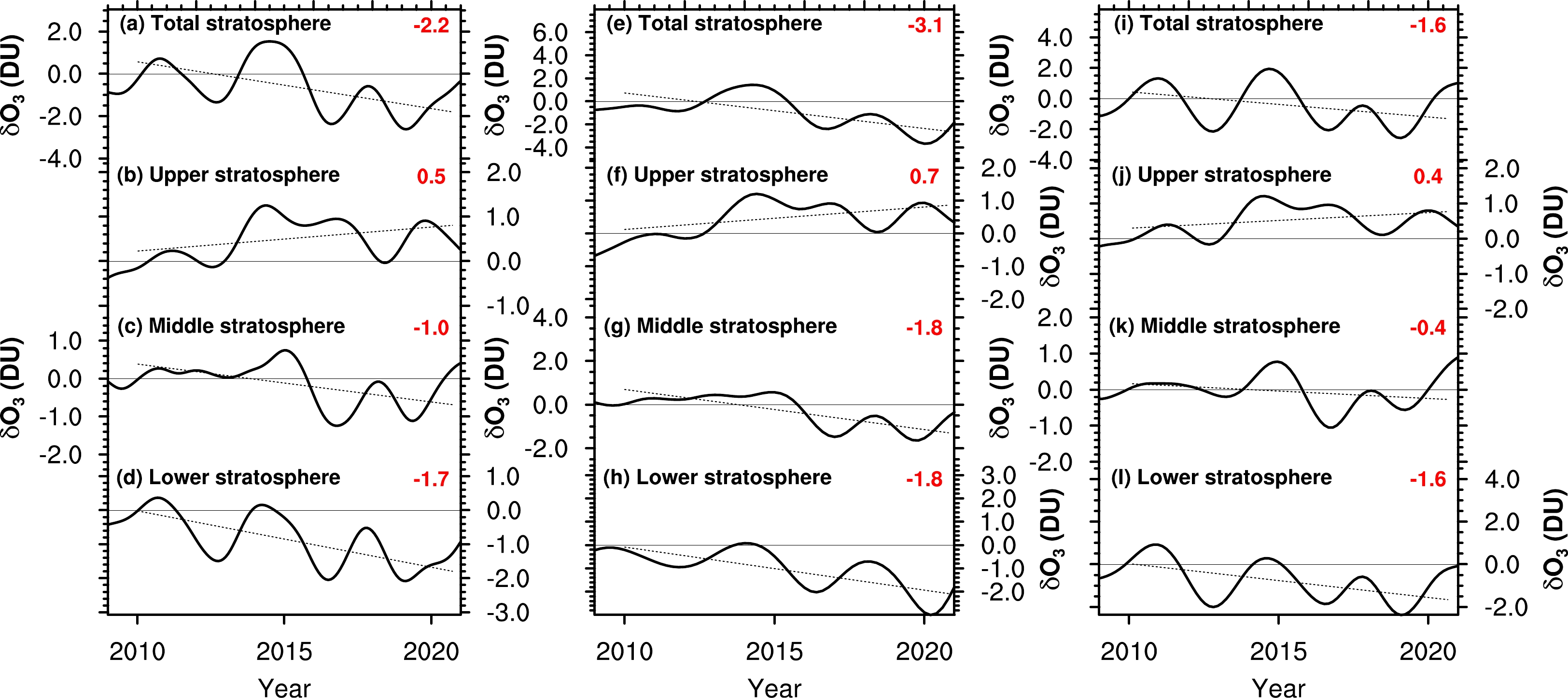
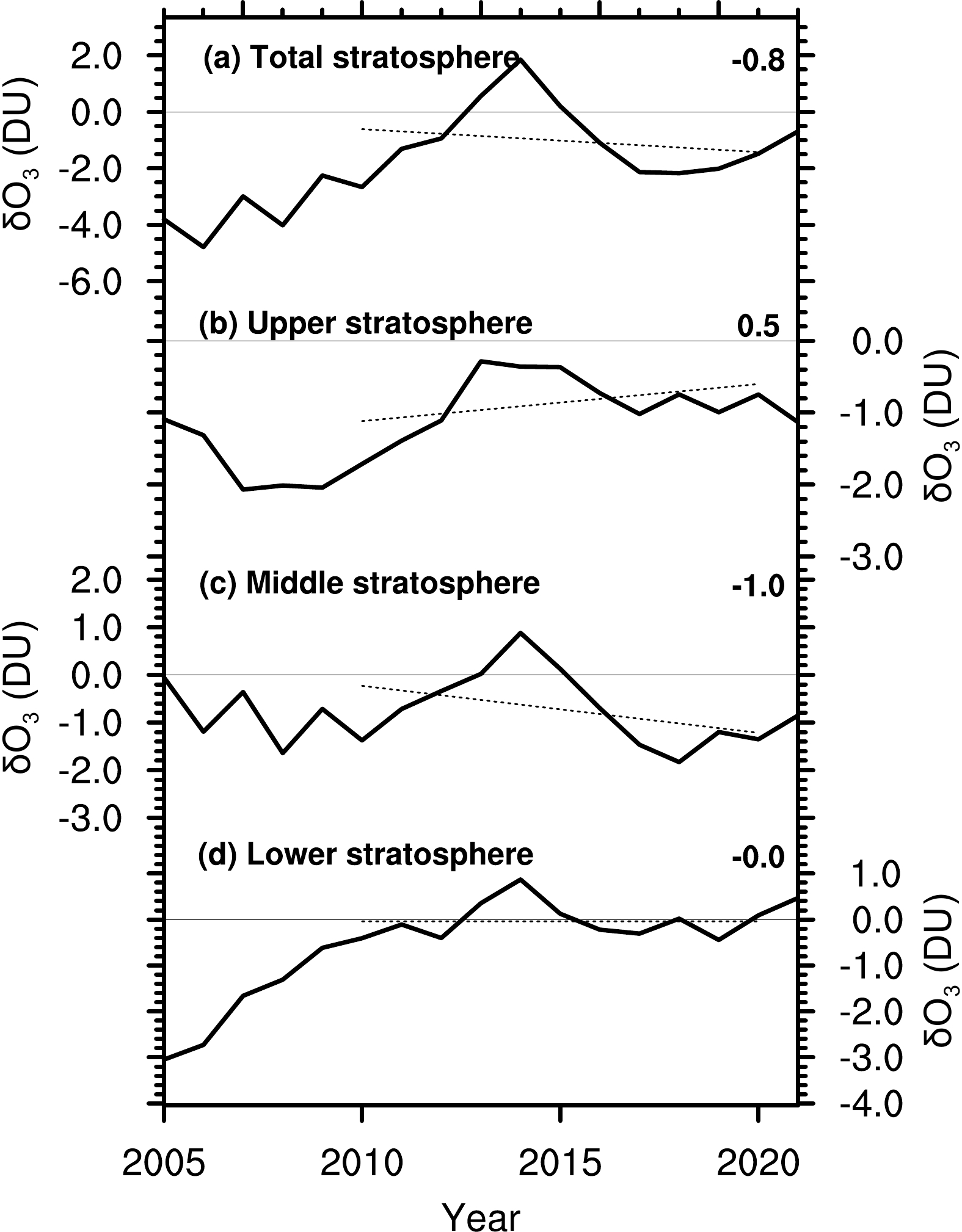
To further understand the TCO changes in Figs. 1 and 3, Figs. 4a–d show the partial column ozone anomalies integrated between different pressure levels of the stratosphere and averaged over 30°S–60°N from 2010 to 2020 based on SWOOSH data. SWOOSH ozone data contain the vertical profile of observed ozone, and the above analysis also shows that its TCO changes are highly consistent with other observational data. From 2010 to 2020, the upper-stratospheric ozone still shows a significant positive trend (Fig. 4b), as seen from 2000 to 2016 (Kyrölä et al., 2013; Ball et al., 2018, 2019; SPARC/IO3C/GAW, 2019); in contrast, the mid-and-lower-stratospheric ozone shows decreasing but non-significant trends from 2000 to 2016 (Kyrölä et al., 2013; Ball et al., 2018, 2019; SPARC/IO3C/GAW, 2019), but from 2010 to 2020 the decreasing trends are strong and significant at the 2σ level (Figs. 4c, d). Figures 4b–d demonstrate that the significant decreasing trends of mid-and-lower-stratospheric ozone jointly contributed to the ozone depletion of the whole stratosphere (Fig. 4a) and the TCO depletion (Figs. 1e, f) from 2010 to 2020.

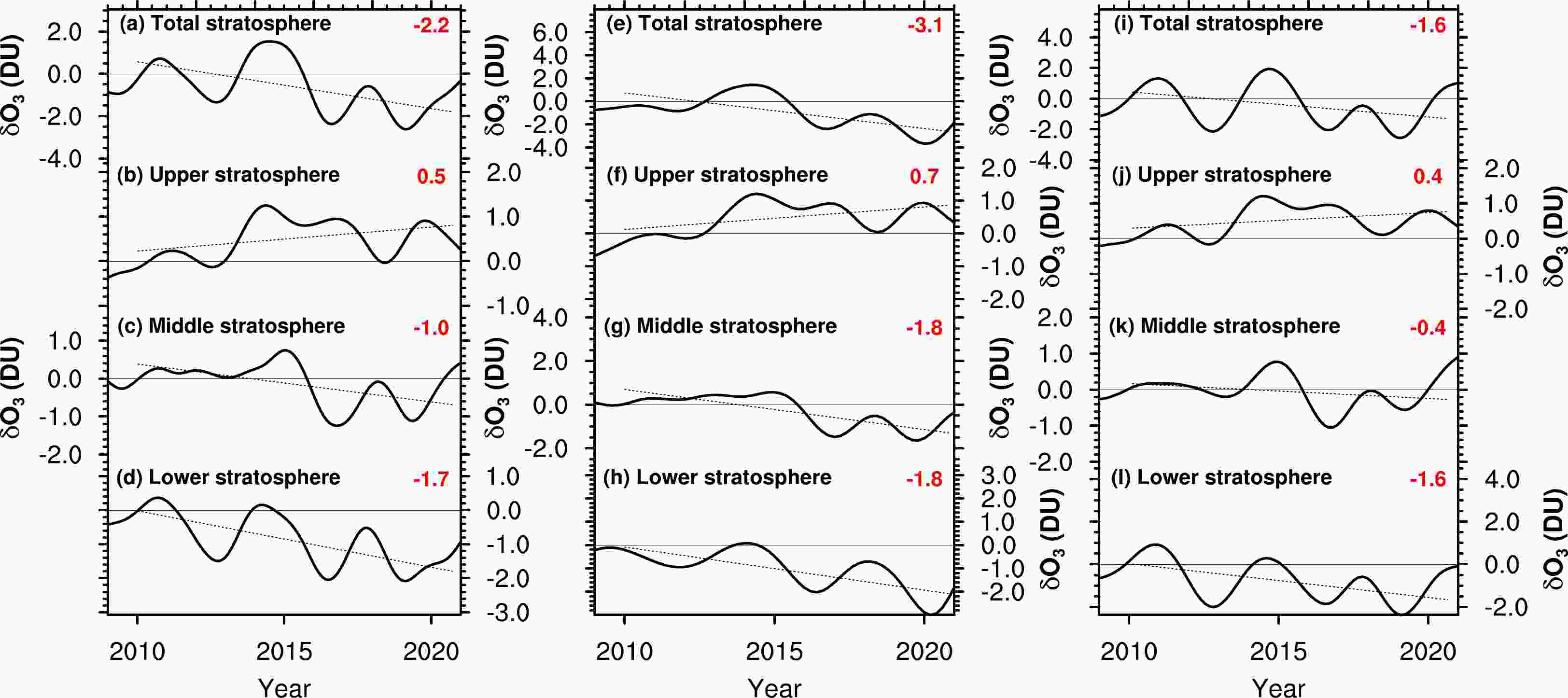
Figure 4.  Partial column ozone trends between different pressure levels from 2010 to 2020 in the 30°S–60°N latitudinal belt. Partial column ozone changes (a, e, i) between 100 and 1 hPa, (b, f, j) between 10 and 1 hPa, (c, g, k) between 32 and 10 hPa, and (d, h, l) between 100 and 32 hPa. The ozone data are from SWOOSH. For data information, please refer to section 2. Panels (a–d) are for 12 months, (e–h) are for May–September, and (i–l) are for October–April. The linear trends (black straight dotted lines) were calculated by linear regression. The number close to the right-y-axis is the linear trend value [units: DU (10 yr)^–1] of TCO changes from 2010 to 2020. Red and black values denote statistical significance and non-significance, respectively, at the 2σ level, using a Student’s t-test. Low-pass filtering (to filter out periods <3 years) was performed on the TCO changes before calculating the trend.

The partial column ozone anomalies integrated between different pressure levels of the stratosphere and averaged over 30°S–60°N from 2010 to 2020 for May–September and for October–April are also shown in Figs. 4e–l. We find that upper (lower) stratospheric ozone is increasing (decreasing) for both May–September (Figs. 4f, h) and October–April (Figs. 4j, l), while the decreasing trend of mid-stratospheric ozone is significant and strong for May–September (Fig. 4g) but non-significant and weak for October–April (Fig. 4k). Since the middle stratosphere is the layer with the largest ozone concentration, the partial column ozone trend for the whole stratosphere is much weaker in October–April compared to that in May–September (Fig. 4e vs. Fig. 4i). Figures 4e–l imply that the decrease in mid-stratospheric ozone for May–September may be the main reason for the decreasing trends of TCO and increasing trends of surface UV being significant and strong from 2010 to 2020 during May–September (Fig. 3) but not in other months.

Figure 5 shows the TCO changes averaged at different latitudes between 60°S to 60°N from 2005 to 2020 for the May–September average based on the TOMCAT/SLIMCAT simulation (see section 2). The results show that the model simulates the recent decreasing trends of TCO since 2010 over the tropics and NH mid-latitudes (Figs. 5b, c) and an increasing trend over SH mid-latitudes (Fig. 5a); however, the decreasing trends are weaker and non-significant compared with the observations (Figs. 5b, c vs. Figs. 1e, f). Figure 6 shows the partial column ozone integrated between different altitudes and averaged over 30°S–60°N from 2005 to 2020 for May–September based on the TOMCAT/SLIMCAT simulation. Consistent with observations (Figs. 4f, g), the model simulates a positive trend for upper-stratospheric ozone and a negative trend for mid-stratospheric ozone (Figs. 6b, c). However, the strongly negative trend of lower-stratospheric ozone in the observed data (Figs. 4d, h, l) is not reproduced by the model (Fig. 6d). Thus, the simulated ozone trend in the whole stratosphere is smaller [–0.8 DU (10 yr)^–1, Fig. 6a], resulting in the simulated decreasing TCO trends over the tropics and NH mid-latitudes being weaker and less significant compared with the observations (Figs. 5b, c vs. Figs. 1e, f).

Figure 5.  TCO changes between different latitudinal belts from 2005 to 2020 for the May–September average based on the TOMCAT/SLIMCAT model experiment, including those between (a) 60°S and 30°S, (b) between 30°S and 30°N, and (c) between 30°N and 60°N. Linear trends (black straight dotted lines) are calculated by linear regression. The number close to the right-hand-y-axis is the linear trend value [units: DU (10 yr)^–1] for 2010–20. Red and black values denote statistical significance and non-significance, respectively, at the 2σ level, using a Student’s t-test. A three-point running average was performed on the TCO changes before calculating the trend.

Figure 6.  Partial column ozone changes between different pressure levels in the 30°S–60°N latitudinal belt from 2005 to 2020 for the May–September average based on the experiment of the TOMCAT/SLIMCAT model. (a) Partial column ozone changes between 100 and 1 hPa, (b) between 10 and 1 hPa, (c) between 32 and 10 hPa, and (d) between 100 and 32 hPa. The linear trends (black straight dotted lines) were calculated by linear regression. The number close to the right-hand-y-axis is the linear trend value [units: DU (10 yr)^–1] for 2010–20. Red and black values denote statistical significance and non-significance, respectively, at the 2σ level, using a Student’s t-test. A three-point running average was performed on the TCO changes before calculating the trend.

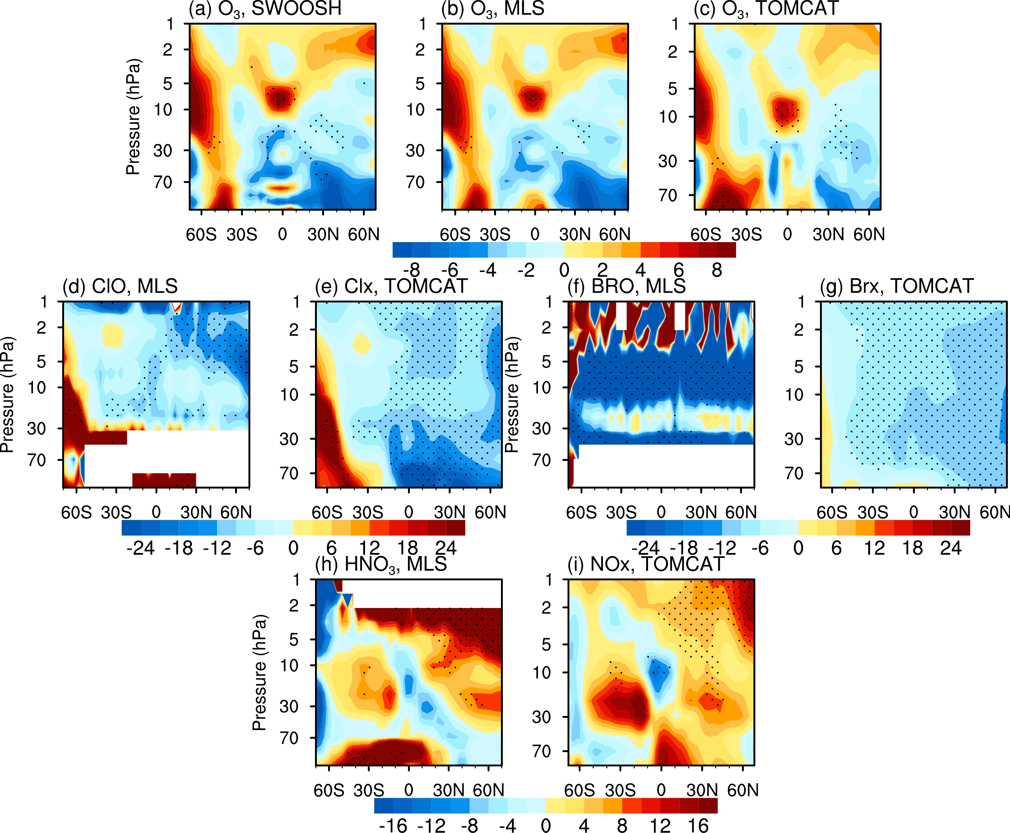
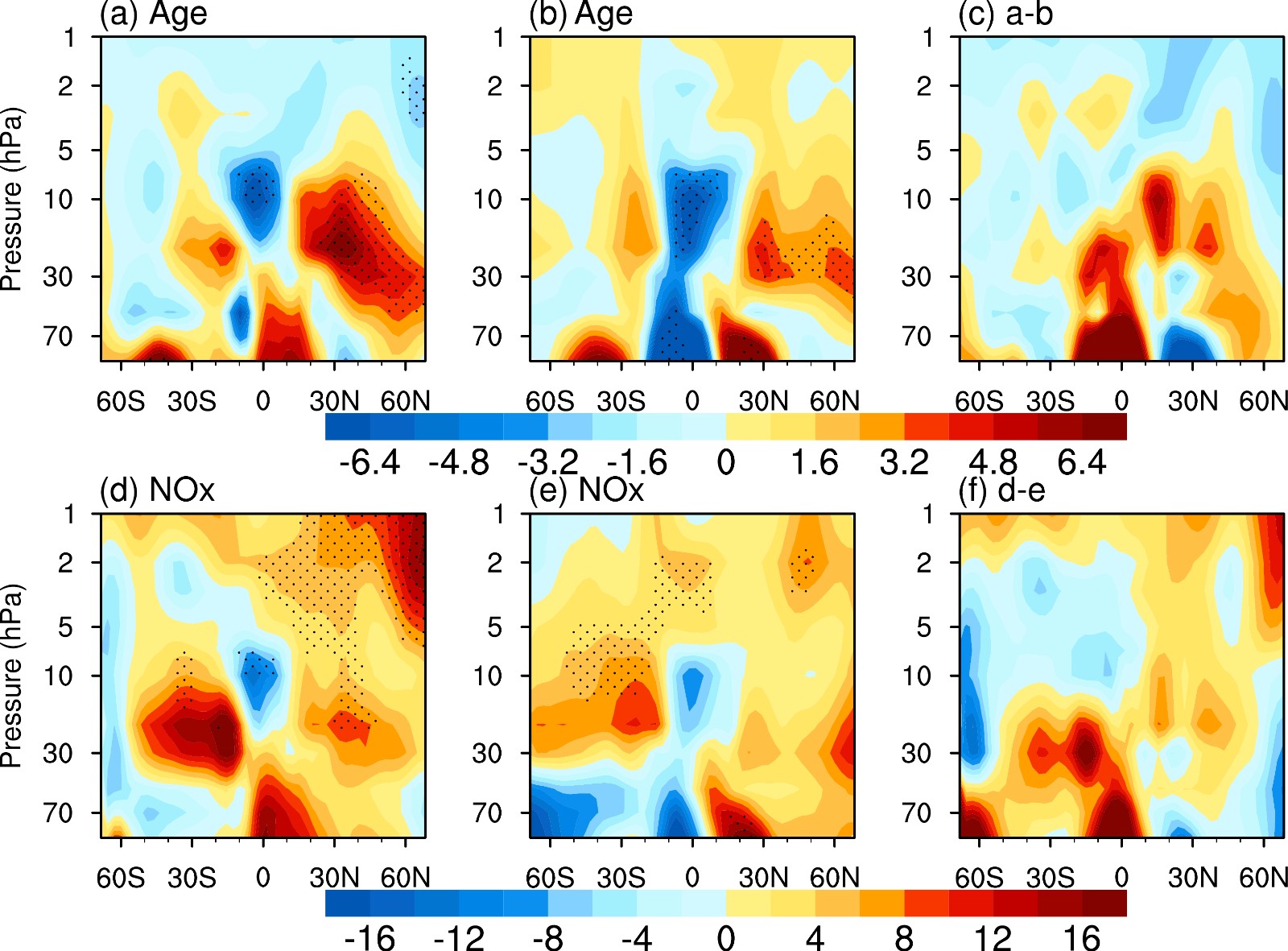
In general, the TOMCAT/SLIMCAT model simulates the recent (since ~2010) ozone trends reasonably well, so the mechanisms responsible for the ozone depletion during 2010–20 are further investigated using both an observational and modeling approach. Figure 7 shows the fractional trends of zonal-mean ozone and the related chemical components from 2010 to 2020 for May–September. We find that ozone exhibits a decreasing trend in most regions of the mid-lower stratosphere (below 10 hPa) in the tropics and NH mid-latitudes. This feature is highly consistent among the SWOOSH data, Microwave Limb Sounder (MLS) data, and the TOMCAT/SLIMCAT simulation (Figs. 7a–c). However, the ozone depletion in the mid-lower stratosphere is much weaker in TOMCAT/SLIMCAT than in the SWOOSH and MLS data, and this explains why the simulated decreasing trends of TCO (Figs. 5b, c) are much weaker than the observations (Figs. 1e, f). Figures 7a–c further corroborate that the significant decrease in mid-and-lower-stratospheric ozone led to the significantly negative trend in the TCO over the tropics and NH mid-latitudes in the past decade (Figs. 1e, f).

Figure 7.  Fractional trend distributions of zonally averaged chemical components for May–September from 2010 to 2020 with respect to the multi-year average. (a–c) O₃; (d) ClO; (e) Cl + ClO; (f) BrO; (g) Br + BrO; (h) HNO₃; (i) NO + NO₂. Panel (a) is from SWOOSH; panels (b, d, f, h) are from the MLS dataset; and panels (c, e, g, i) are from the TOMCAT/SLIMCAT simulation. The fractional trend was calculated by the linear trend divided by the average [units: % (10 yr)^–1]. Linear trends were calculated by linear regression. Low-pass filtering (to filter out periods <3 years) was performed on the chemical component changes before calculating the trend. The dotted area indicates statistical significance at the 2σ level based on a Student’s t-test.

Active chlorine (Cl_x = Cl + ClO + Cl₂O₂) and bromine (Br_x = Br + BrO) are the most important ozone-depleting chemical components. Figures 7d–g show the Cl_x and Br_x linear trends from 2010 to 2020 for May–September based on MLS data and the TOMCAT/SLIMCAT simulation. For the upper stratosphere, Cl_x (Cl₂O₂ excluded) and Br_x decreased from 2010 to 2020, which would be conducive to upper stratospheric ozone recovery but cannot explain the decreasing mid-stratospheric ozone. For the lower stratosphere, ClO is increasing in the MLS data (Fig. 7d). The increase in ClO agrees with the strong ozone depletion in the lower stratosphere in the SWOOSH and MLS data (Figs. 7a, b). The TOMCAT/SLIMCAT simulation shows different results from MLS (Figs. 7d, e). In particular, Cl_x decreases significantly in the lower stratosphere in TOMCAT/SLIMCAT (Fig. 7e), and the ClO in the TOMCAT/SLIMCAT simulation also has the same characteristics (not shown). This explains why the magnitude of the ozone decline in the lower stratosphere is much smaller in TOMCAT/SLIMCAT (Fig. 7c) than in the SWOOSH and MLS data (Figs. 7a, b) and also implies that Cl_x may have been the cause of the lower stratospheric ozone reduction after 2010. The increase in Cl_x in the lower stratosphere may be related to increased emissions of short-lived chlorine source gases not considered in the model; however, these aspects are not further discussed in the present paper.

It is found that stratospheric NO_x increases significantly in the tropics and NH mid-latitudes, especially over 30°S–60°N, from 2010 to 2020 (Figs. 7h, i). In Fig. 7h, we replace the changes in NO_x with observed HNO₃ because HNO₃ is a major reservoir of NO_x in the stratosphere, and an increase in HNO₃ can serve as a good proxy of any increase in NO_x. NO_x can react to deplete stratospheric ozone (Crutzen, 1970) and is considered to be one of the important factors affecting ozone recovery (Chipperfield, 2009; Ravishankara et al., 2009). Note that the spatial patterns in Figs. 7h, i are closely consistent with those in Figs. 7a–c in the middle stratosphere, which implies that increasing NO_x may be the main reason for the decrease in mid-stratospheric ozone. In summary, according to the above analyses, the decrease in mid-stratospheric ozone may be the main reason for the decreasing trend of TCO and increasing trend of surface UV being significant and strong from 2010 to 2020 for May–September. Additionally, the increase in NO_x during May–September likely played a key role in influencing the significant decreasing trend of mid-stratospheric ozone.

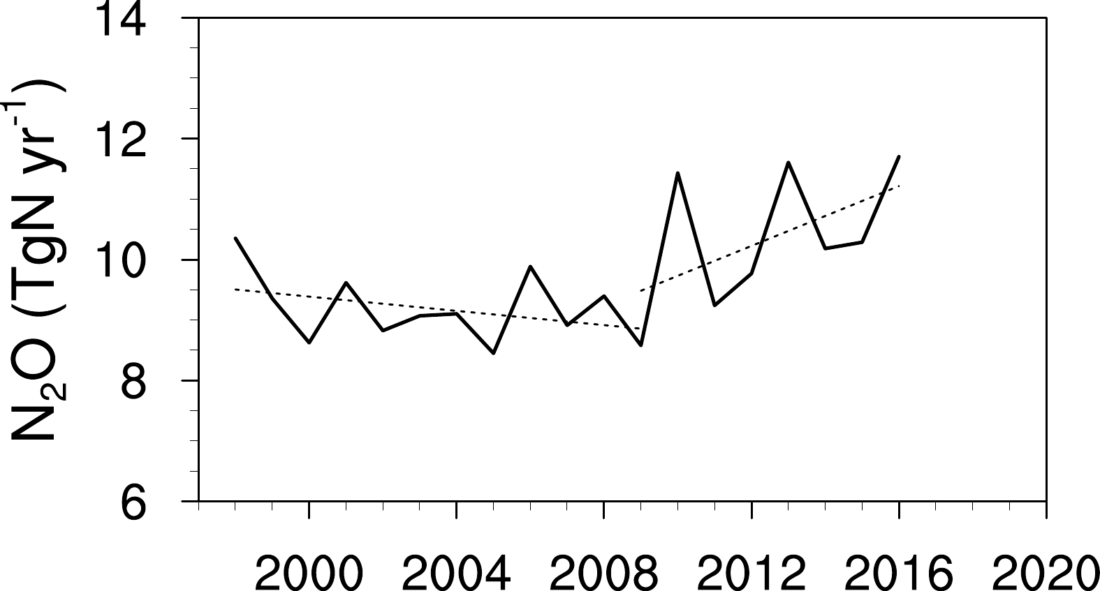
One more issue of interest is why the mid-stratospheric ozone depletion, or, for example, the increase in NO_x, mainly occurred in the tropics and NH mid-latitudes after 2010 for May–September. Nitrous oxide (N₂O) is highly stable in the troposphere until it is transported into the stratosphere, where its chemical decomposition is the primary source of stratospheric NO_x (Chang, 2003). Previous studies have pointed out that the increase of N₂O mainly influences mid-stratospheric ozone (Chipperfield, 2009; Ravishankara et al., 2009). It is important to note that global N₂O emissions accelerated substantially after 2009 (Thompson et al., 2019) (Fig. 8), which may be the reason for the significant increase in stratospheric NO_x after 2010. On the other hand, the chemical decomposition of N₂O is also related to the strength of the stratospheric circulation. Weakened meridional transport with older air is characterized by a larger relative conversion of N₂O into NO_x. Figure 9 shows the fractional trends of the age-of-air for May–September and for October–April based on the TOMCAT/SLIMCAT simulation from 2010–20. Clearly, the trends in the age-of-air for May–September are larger than those for October–April in the middle stratosphere over 30°S–60°N, from 2010 to 2020 (Figs. 9a–c). The larger (smaller) trends of the age-of-air correspond to larger (smaller) trends of NO_x (Figs. 9d–f) in the middle stratosphere, which helps to explain why the mid-stratospheric ozone depletion mainly occurred during May–September.

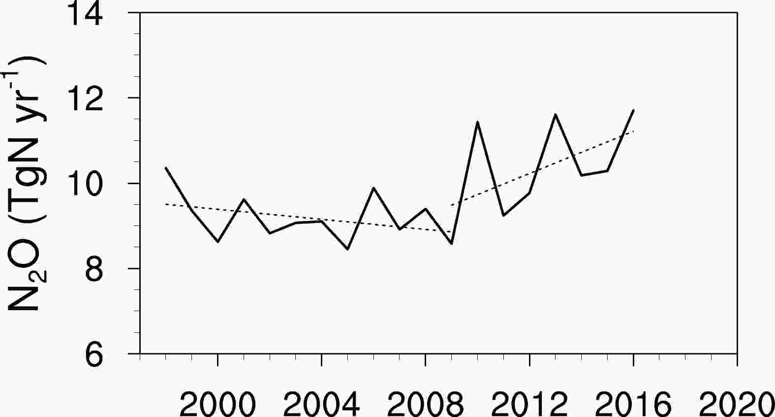
Figure 8.  Annual averaged global surface N₂O emissions. Linear trends (black straight dotted lines) are calculated by linear regression for 1998–2009 and 2009–16. For details on the surface N₂O emissions data, please refer to Thompson et al. (2019).

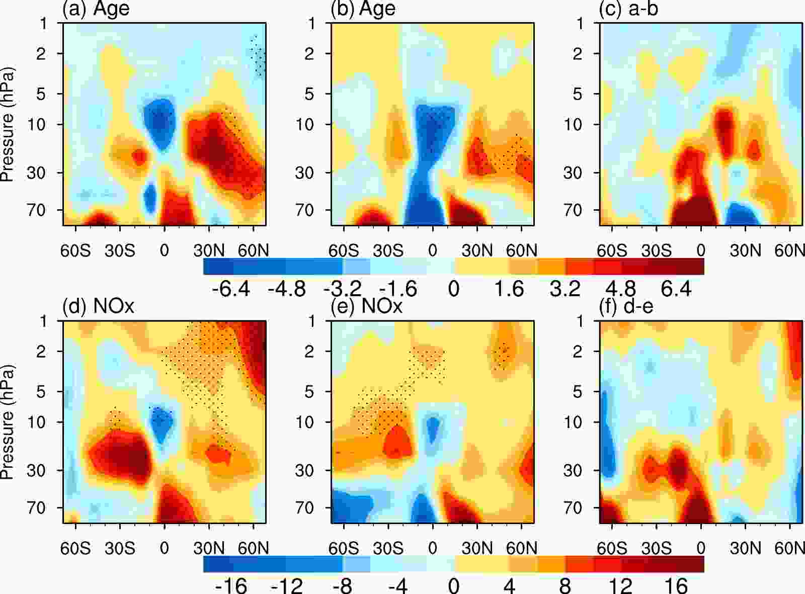
Figure 9.  Fractional trend distributions of the zonally averaged age-of-air and NO_x from 2010 to 2020 based on the experiment of the TOMCAT/SLIMCAT model. (a, b) Age-of-air and (d, e) NO + NO₂ for (a, d) May–September (b, e) and October–April. Panels (c) and (f) show the seasonal differences. The fractional trend was calculated by the linear trend divided by the average [units: % (10 yr)^–1 ]. Linear trends were calculated by linear regression. Low-pass filtering (to filter out periods <3 years) was performed on the chemical component changes before calculating the trend. The dotted area indicates statistical significance, at the 2σ level, based on a Student’s t-test.

This study finds that surface UV radiation in the tropics and NH mid-latitudes shows a statistically significant increasing trend, at the 2σ level, from 2010 to 2020 for May–September due to the beginning of TCO depletion. The significant decreasing trends of lower- and mid-stratospheric ozone jointly contributed to the TCO depletion from 2010 to 2020, and the decrease in mid-stratospheric ozone for May–September may be the main reason for the decreasing trends of TCO being significant and strong from 2010 to 2020 during May–September but not during other months. The increase in N₂O emissions after 2009 and weakened mid-stratospheric circulation for May–September may have caused the increasing NO_x in the stratosphere, resulting in the mid-stratospheric ozone being significantly depleted after 2010 for May–September. Since N₂O is the primary source of stratospheric NO_x, our results further support those predicted in previous studies (Randeniya et al., 2002; Chipperfield, 2009; Ravishankara et al., 2009), i.e., that N₂O emissions delay ozone recovery. More importantly, this study demonstrates that N₂O emissions not only delay the future recovery of ozone but even lead to a depletion in TCO and an increase in surface UV radiation in May–September over the tropics and NH mid-latitudes commensurate with global warming. This unexpected ozone depletion and UV increase can potentially pose more serious threats (including an increased incidence of skin cancers and ecological damage) than at the poles since the tropics and NH mid-latitudes are densely populated and economically developed regions.