The Probability Density Function Related to Shallow Cumulus Entrainment Rate and Its Influencing Factors in a Large-Eddy Simulation

Cumulus clouds have important effects on the vertical transport of heat, moisture, and momentum and play an important role in affecting the energy budget of the Earth–atmosphere system and climate change (Guo et al., 2014, 2015b; Donner et al., 2016; Wang et al., 2018; Yang et al., 2019; Jeyaratnam et al., 2021; Sheng et al., 2022). In weather and climate models, because model grid spacing is insufficient to resolve convective processes, the parameterization of cumulus clouds must be achieved using empirical hypotheses and physical variables at grid points (Zhang and McFarlane, 1995; Lin et al., 2000; Donner et al., 2001; Wu, 2012; Xie and Liu, 2013). The quality of the cumulus parameterization scheme is crucial for simulating precipitation, monsoons, Madden-Julian oscillations, and tropical cyclones (Zou and Zhou, 2011; Del Genio et al., 2012; Yang et al., 2015; Wang et al., 2017; Zhao et al., 2018a). Entrainment-mixing between cumulus clouds and ambient air is a key process that affects cloud development and the formation of precipitation, by causing cloud droplet evaporation to alter temperature, humidity, buoyancy (B), and vertical velocity (w) in clouds (Jonas, 1990; Houze, 1993; Telford, 1996; de Rooy et al., 2013; Yeom et al., 2017; Wang, 2020; Luo et al., 2022; Wang et al., 2023). In many cumulus parameterization schemes, the lateral entrainment rate (λ) is a physical variable characterizing the strength of entrainment, which has a significant influence on climate sensitivity, precipitation, and monsoons (Klocke et al., 2011; Yang et al., 2013, 2021; Zhao, 2014; Lu and Ren, 2016; Hanf and Annamalai, 2020).

To better understand the process of entrainment-mixing and improve cumulus parameterization schemes in models, an accurate calculation of λ is essential. Stommel (1947) first calculated λ using the temperature and specific humidity inside and outside the cloud. Based on this, Yanai et al. (1973) and Betts (1975) proposed the bulk-plume method to calculate λ according to conserved physical variables (i.e., total moisture, liquid water potential temperature (θ_l), and moist static energy) in clouds and ambient air. The bulk-plume method has been used in many studies. For example, Esbensen (1978) used this method to calculate the observed λ in large-scale shallow cumulus clouds, and this was also applied to calculate λ from aircraft observations (Neggers et al., 2003; Gerber et al., 2008; Lu et al., 2018) and satellite data (Luo et al., 2010; Takahashi and Luo, 2012; Li et al., 2022; Takahashi et al., 2023). Romps (2010) proposed a method to estimate λ by directly calculating the amount of air entrained into the cloud in large-eddy simulation (LES) experiments and found that the results were approximately twice those from the bulk-plume method. Dawe and Austin (2013) noted that the reason for the difference may be related to the presence of a moist cloud shell around the cloud core that is more humid than the ambient air. Nevertheless, accurately calculating λ remains a challenge, hindering the improvement of cumulus parameterization schemes.

The parameterization of λ is an important way to describe the process of entrainment-mixing in models (de Rooy et al., 2013; Lu et al., 2016; Zhang et al., 2016; Villalba-Pradas and Tapiador, 2022). However, the process of entrainment-mixing is also often considered to be a stochastic process. Romps and Kuang (2010) found that a parcel model with a constant or continuous λ could not reproduce the observed variability of clouds, whereas a stochastic parcel model could, in which entrainment behaves like a stochastic Poisson process. Observations have shown that the probability density functions (PDFs) of λ for shallow and deep convection follow a log-normal distribution (Lu et al., 2012a; Guo et al., 2015a), supporting the stochastic process of entrainment-mixing. Romps and Kuang (2010) and Romps (2016) presented Lagrangian and Eulerian implementations of the stochastic parcel model, respectively, to treat the process of entrainment-mixing in cumulus clouds as a stochastic process. Böing et al. (2014) studied the process of entrainment-mixing using two parcel models that describe λ in different ways. The stochastic mixing model with λ satisfying a gamma distribution better captured the scatter of the in-cloud thermodynamic properties. Yang et al. (2021) linked the mass fluxes between shallow and deep convection by assuming that λ satisfies a log-normal distribution, and a modified deep convection scheme improved precipitation simulations in mean state and variability at various timescales. However, a simply assumed log-normal distribution of λ may cause uncertainty since this assumption only considers statistical characteristics. Therefore, analyzing the PDF of λ and its influencing factors provides an important reference for numerical models to improve cumulus parameterization schemes.

Despite significant progress, further improvement of the calculation accuracy of λ and determination of the PDF of λ and its influencing factors remain worthy of further study. This study developed an improved bulk-plume method and applied it to a simulated cumulus cloud case using an LES. First, the accuracy of the method for calculating λ was evaluated. Second, the PDFs of λ were fitted to a log-normal distribution, then the variation in the fitting parameters over time and the influencing factors were analyzed. Finally, the variation in the PDFs of λ with height was analyzed. The LES was chosen because it is difficult to obtain the PDFs of λ at different heights and times owing to limitations to aircraft observations. An LES can provide the three-dimensional structure of cumulus convection and its temporal evolution (Neggers et al., 2003; Endo et al., 2015), which provides important data for studying λ (Romps, 2010; Dawe and Austin, 2013; Drueke et al., 2019).

The remainder of this paper is organized as follows. Section 2 introduces the model setting and simulation results. Section 3 describes and verifies the improved method for calculating λ. Section 4 analyzes the spatial and temporal distribution of λ, the variation in PDFs of λ with time and height, and its influencing factors. The conclusions and discussions are presented in section 5.

The LES model was used to simulate cumulus clouds over the Southern Great Plains (SGP) during the LES Atmospheric Radiation Measurement Symbiotic Simulation and Observation (LASSO) experiment (Gustafson et al., 2020) on 11 June 2016 [Coordinated Universal Time (UTC) and Local Standard Time (LST, LST = UTC – 6)] (Xu et al., 2022). The model adds time-varying large-scale forcing (Endo et al., 2015) to a Weather Research and Forecasting model tailored for solar irradiance forecasting (WRF-Solar), which can better handle radiation-related processes, as well as cloud-aerosol-radiation feedback (Haupt et al., 2016; Jimenez et al., 2016). The large-scale forcing data and model settings were the same as those used by Xu et al. (2022). The horizontal grid spacing of the model was 100 m × 100 m, the number of grids was 144 × 144, and the vertical grid spacing was 30 m with 225 layers. The simulation started at 1200 UTC on 11 June 2016, and ended at 0300 UTC on 12 June 2016. The output of simulation results occurred every 10 minutes. The quasi-steady state in an LES may be reached within a few large-eddy turnover times (Moeng and Sullivan, 1994; Nakanish, 2001). Here, the spin-up time was set to 3 h (Xu et al., 2022), which was more than eight large-eddy turnover times. The chosen microphysical scheme was the Thompson aerosol-aware scheme (Thompson and Eidhammer, 2014) with an improved parameterization of the entrainment-mixing mechanism (Luo et al., 2020; Xu et al., 2022).

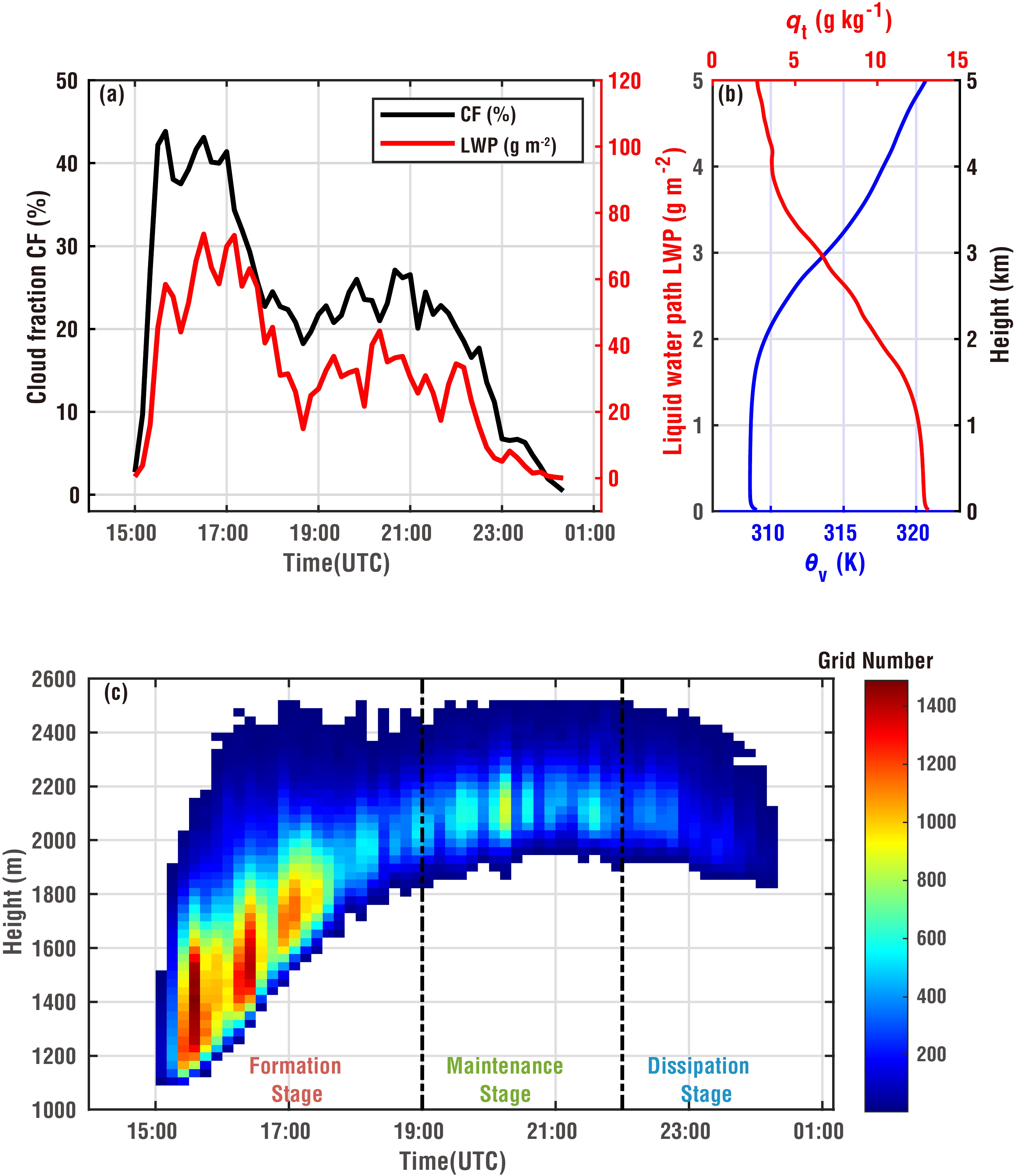
For this cumulus cloud case, the diurnal variations of the simulated cloud fraction (CF) and liquid water path (LWP) in Fig. 1a illustrate a first peak around 1600–1700 UTC and a secondary peak around 2000–2100 UTC. Since LWP is a vertically integrated quantity and CF is a horizontal coverage value, the peak timings of the two variables do not always coincide (Shin et al., 2021). The mean thermodynamic profiles (Fig. 1b) show that the mean characteristics of the convective planetary boundary layer are as follows: the surface layer from 0 m to about 330 m, the mixed layer from about 330 m to 1600 m, and the inversion layer from about 1600 m to 2800 m. The maximum updraft in the simulation is 9.40 m s^–1, and the mean of the maximum updraft for each moment is 6.19 m s^–1. The simulated cumulus clouds formed at approximately 1500 UTC and dissipated completely at approximately 2400 UTC. The simulations generally captured the diurnal variation of cumulus clouds (Xu et al., 2022).

Figure 1.  (a) Time series of the cloud fraction (CF) and liquid water path (LWP) from the simulation on 11 June 2016. (b) The simulated mean thermodynamic profiles of virtual potential temperature (θ_v) and total water vapor mixing ratio (q_t). (c) Distribution of the grid numbers of cloud grid points with time and height. The black, dash-dotted lines divide the three stages of cloud ensemble evolution: formation (1500–1900 UTC), maintenance (1900–2200 UTC), and dissipation (2200–0020 UTC the next day). The blank values in (c) indicate that no grid point of the area meets the criteria for a non-precipitating cloud.

Cloud grid points without precipitation were selected based on the following criteria: their liquid water mixing ratios (q_l) must exceed 0.01 g kg^–1, B must be greater than 0 m s^–2, and rain-water mixing ratios must be less than 0.005 g kg^–1 (Lu et al., 2012b). Figure 1c shows the time-height distribution of the number of cloud grid points in the simulated region. For the case of cumulus cloud, the height of the cloud base continued to rise from 1500 to 1900 UTC, and the cloud ensemble vigorously developed within a large number of cloud grids, accompanied by the decay of small cumulus clouds and the appearance of new clouds; after 1900 UTC the number of cloud grid points declined and after 2200 UTC the cumulus cloud ensemble gradually dissipated. Based on the temporal and spatial distribution characteristics, the simulated cumulus clouds were divided into three stages: formation (1500–1900 UTC), with continuous increases in cloud base and top heights, maintenance (1900–2200 UTC), with relatively consistent cloud base and top heights, and dissipation (2200–0020 UTC the next day), with decreasing cloud base and top heights.

The parameter λ can be calculated using the bulk-plume method (Betts, 1975; Neggers et al., 2003; Gerber et al., 2008):

where $\phi $ is a conserved physical variable during cloud ascent, the subscripts c and e represent the cloud and ambient air, respectively, and z is height. Substituting the total water mixing ratio (q_t) and θ_l as the conserved variables into Eq. (1) yields:

The total water vapor mixing ratio is defined as:

where q_v is the water vapor mixing ratio. θ_l is defined as (Betts, 1973):

where θ = γT is the potential temperature with γ = (p₀ / p)^0.286; p₀ and p are standard atmospheric pressure and air pressure, respectively; T is temperature; L_v is latent heat; and c_p is the specific heat capacity at constant pressure.

Substituting Eq. (4) and Eq. (5) into Eq. (2) and Eq. (3) yields:

where q_vc in the cloud is the saturated water vapor mixing ratio calculated according to the Clausius-Clapeyron equation (Wallace and Hobbs, 2006). The q_le cancels and does not appear in Eq. (6) considering the nature of ambient air. Combining Eqs. (6) and (7) with q_lc in the cloud at different heights and meteorological properties of ambient air, both T_c and λ in the cloud can be calculated simultaneously by iteration. Note that the input variables of this method are q_lc in the cloud and q_ve, T_e, and p_e of ambient air; the output variables are q_vc, T_c, and λ; and the remaining variables are intermediate variables.

The improved method does not depend on which conserved variable is used to calculate λ. On the contrary, the iteration of the two equations takes into account the simultaneous conservation of the two physical variables, making the calculation of λ more accurate. For cumulus clouds with multi-layer data (in this study referring to LES simulations), λ is calculated layer-by-layer from the cloud base to the cloud top, allowing for the vertical distribution of λ to be obtained.

The variables required to calculate λ from the model results were determined as follows: First, the domain-averaged q_ve, T_e, and p_e were taken as the properties of the ambient air involved in the process of entrainment-mixing (Lu et al., 2012b). Second, an average q_lc of the cloud grid points with positive B (the virtual potential temperature in the cloud exceeds that of the environment) in each layer of the domain was considered as the cloud properties of that layer. Finally, the cloud base height at each moment was the lowest height of the cloud grid points in the domain at that moment.

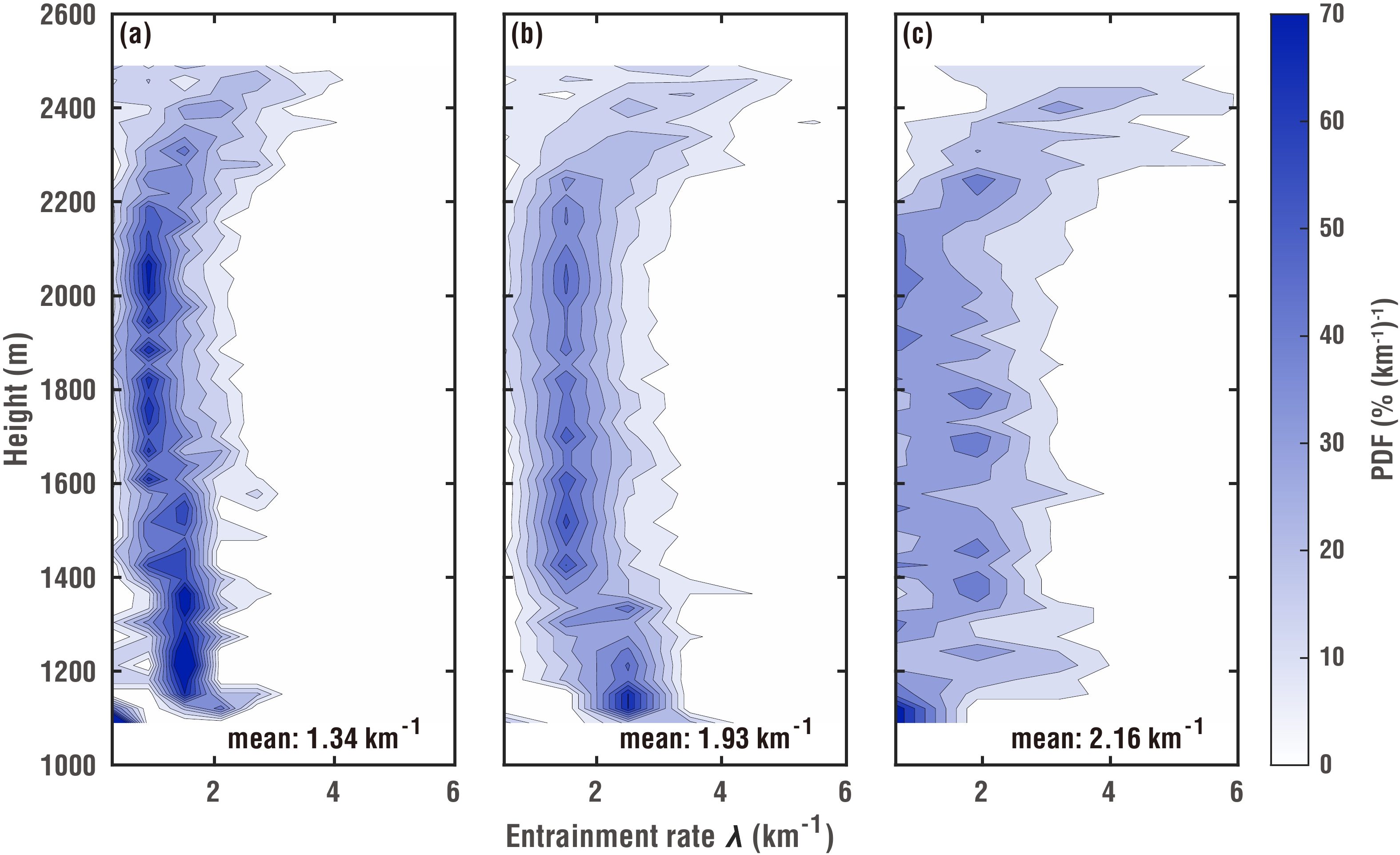
Before analyzing λ, as calculated using the improved method, it is necessary to examine the accuracy of the improved method with respect to the bulk-plume method. Figure 2 compares the PDF of λ calculated by the improved method described in section 3.1, with that calculated by the traditional bulk-plume method [Eqs. (2) and (3)]. The results show that λ calculated by the improved method was relatively large in the lower layers, decreased gradually with increasing height, and increased gradually in the upper layers (Fig. 2b). The λ calculated from the traditional bulk-plume method using q_t was smaller than that calculated using the same method but with θ_l. Interestingly, λ from the improved method was between those of the traditional method using q_t or θ_l. The mean value of λ calculated by the improved method was 1.93 km^–1, and the mean value of λ calculated from q_t and θ_l was 1.34 km^–1 and 2.16 km^–1, respectively. Therefore, the improved method can reduce the uncertainty associated with traditional methods.

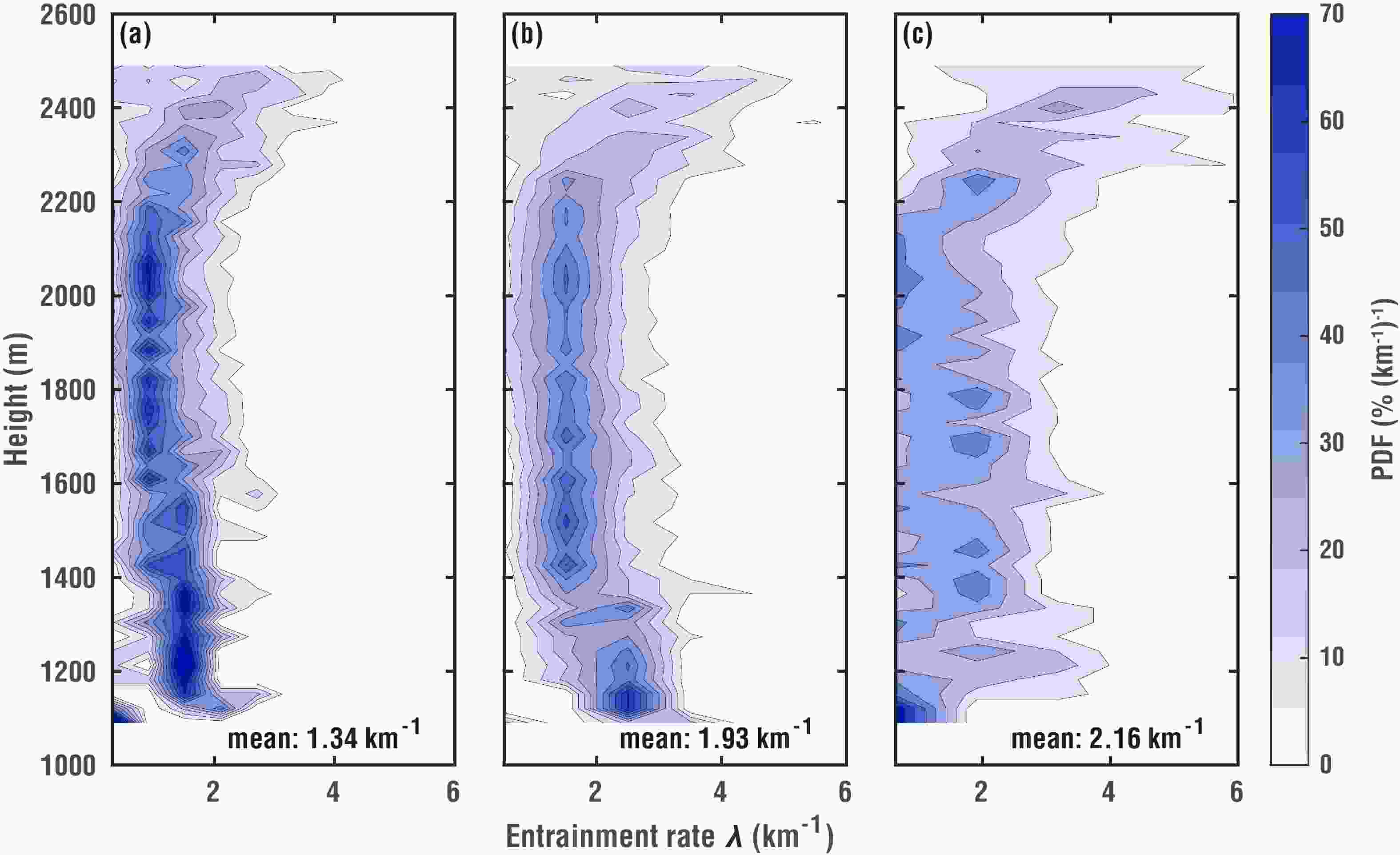
Figure 2.  Probability density function (PDF) of entrainment rate (λ) as a function of height calculated using (a) the bulk-plume method using total water mixing ratio (q_t), (b) the improved method, and (c) the bulk-plume method using liquid water potential temperature (θ_l). The mean values of λ calculated by the three methods are shown in the figure.

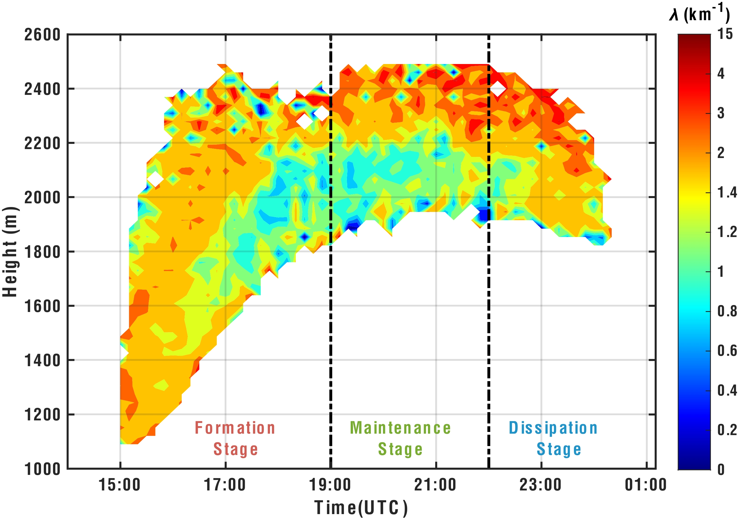
Figure 3 shows the spatial and temporal distributions of λ after examining the accuracy of the improved method for calculating λ. In the formation and dissipation stages, λ exceeded that in the maintenance stage, that is, λ decreased at first and then increased with time. In the vertical direction, λ was generally large in the lower and upper layers, but smaller in the middle layers. The average profile of λ also demonstrates that λ first decreased and then increased along with the increase in height (Fig. 2b) and the overall vertical distribution of λ that decreased with height was consistent with that obtained in previous studies (Dawe and Austin, 2013; Xu et al., 2021). However, λ exhibited some differences at different stages of the cumulus ensemble life cycle. During formation, λ was relatively large near the cloud base and initially decreased before increasing with increased height. During the maintenance stage, the vertical distribution of λ was relatively consistent, and the overall trend featured a decrease of λ with increasing height and then increasing, whereas λ in the middle layer (~2000–2200 m) changed only slightly with height. During dissipation, λ increased with increasing height.

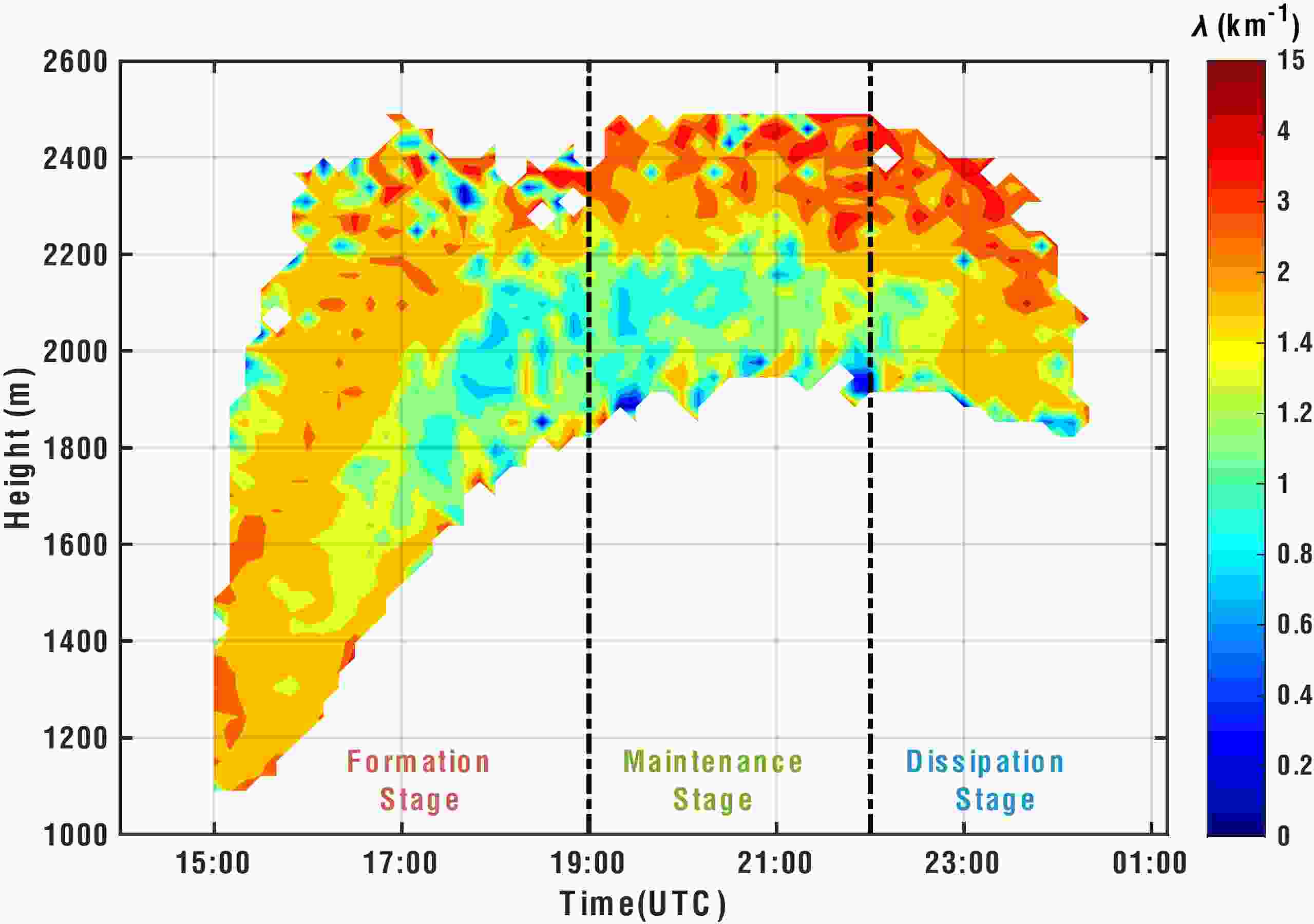
Figure 3.  Distribution of entrainment rate (λ) with time and height. The black dash-dotted lines divide the three stages of cloud ensemble evolution: formation (1500–1900 UTC), maintenance (1900–2200 UTC), and dissipation (2200–0020 UTC the next day). The blank values indicate that no grid point of the area meets the criteria for a non-precipitating cloud.

In the formation stage, the cloud ensembles experienced significant λ over a large depth due to the rapid development accompanied by the decay of small cumulus clouds and the appearance of new clouds, some of which were initial cumulus clouds; the main reason is that the cloud ensemble in the formation stage possessed a smaller w than the subsequent maintenance stage [Fig. S1b in the electronic supplementary material (ESM)] since λ frequently increases with decreasing w (Neggers et al., 2002; de Rooy et al., 2013; Lu et al., 2016; Xu et al., 2021) and λ has the strongest relationship with w among other thermodynamic/dynamical properties (see sections 4.2.2 and 4.3.2 for detailed analysis). In contrast, the larger w in the maintenance stage (Fig. S1b in the ESM) leads to the development of smaller λ in the lower part of the cloud (Fig. 3). The cloud dissipation was responsible for the increasing λ near cloud tops and toward the end of the simulation, as the dissipating clouds share similar physical properties with the ambient air [resulting in small $\phi_{\rm{e}} $ – $\phi_{\rm{c}} $ in Eq. (1)]. It is also worth noting that smaller w occurred in the cloud ensembles near the cloud tops and toward the end of the simulation (Fig. S1b; in the ESM), resulting in larger λ (Fig. 3). The increasing λ towards the cloud top has been found in many model simulations (Romps, 2010; Dawe and Austin, 2011, 2013; Xu et al., 2021).

Dawe and Austin (2013) diagnosed the spatial and temporal distributions of λ for each individual shallow cumulus cloud using a cloud-tracking algorithm in an LES. The results for one of the cumulus clouds showed that λ was larger in the lower levels and gradually decreased with height, and there were several large values in the upper layers. Note that λ initially decreased and then increased with time. The spatial and temporal distributions of the cumulus ensemble in the present study represented the ensemble characteristics of all individual cumulus clouds and were very similar to the results of individual cumulus clouds in Dawe and Austin (2013). This indicates that the spatial and temporal distributions of the cumulus ensemble λ simulated in this study can also represent the characteristics of individual cumulus clouds. In addition, the variation with height in PDF of λ across all cumulus clouds simulated by Dawe and Austin (2013) demonstrated that ensemble λ initially decreased and then increased with height, consistent with the vertical variation of ensemble λ simulated in the present study.

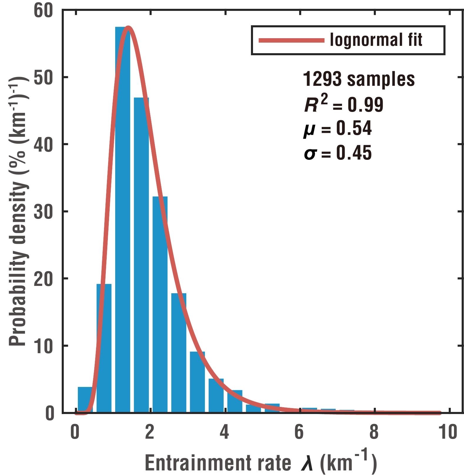
Figure 4 shows the PDF of 1293 domain-averaged λ values at all heights and times. Due to the assumptions described in section 3.2, we note that the calculated λ is the cloud ensemble λ. The entrainment characteristics of cloud ensembles (e.g., cloud ensemble λ) are required in current general circulation models (GCMs) (Dawe and Austin, 2013). The PDF of λ was well fitted using a log-normal distribution (coefficient of determination R² = 0.99); similar results were obtained by Lu et al. (2012a). The log-normal distribution was chosen as the fitting function because previous studies have demonstrated that the PDF of λ conforms to a log-normal distribution (Lu et al., 2012a; Dawe and Austin, 2013; Guo et al., 2015a). In climate models, the grid spacing is coarse and cumulus convection is often described through parameterization. The different effects of entrainment on cumulus convection can be obtained by parameterizing λ rather than by assuming a constant λ (Gregory, 2001; Neggers et al., 2002; Wu, 2012). Therefore, a wide distribution of λ is reasonable. It is also important to treat the process of entrainment-mixing as a stochastic process (Romps and Kuang, 2010; Böing et al., 2014; Romps, 2016; Yang et al., 2021). The PDF of λ is well described by the log-normal distribution (Fig. 4), which supports stochastic entrainment and has important implications for treating convection in models.

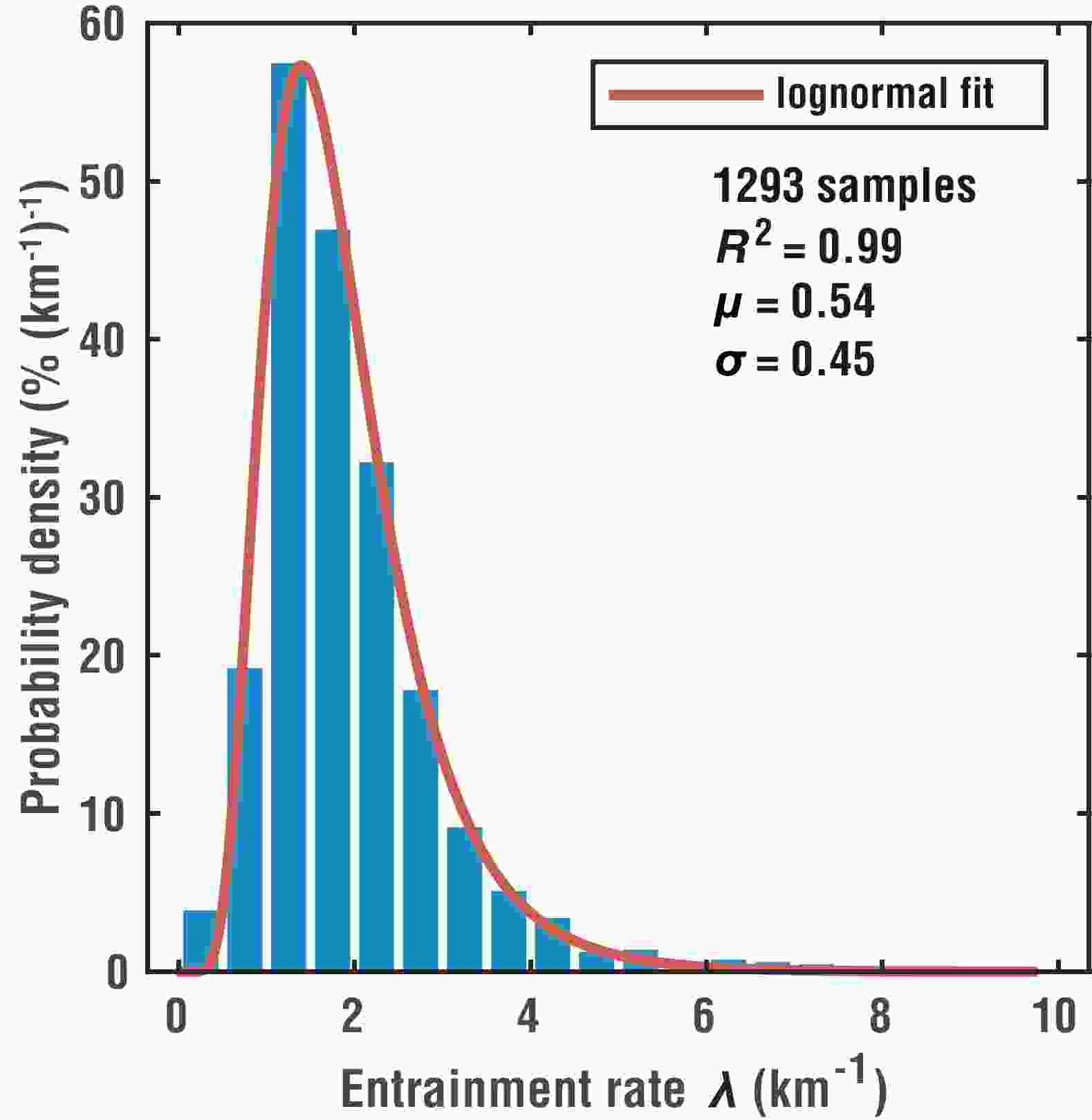
Figure 4.  Probability density function of the entrainment rate (λ) at all times and heights. The number of samples, the coefficient of determination (R²), mean (μ), and standard deviation (σ) of ln(λ) for the log-normal fit (red line) of all data are provided.

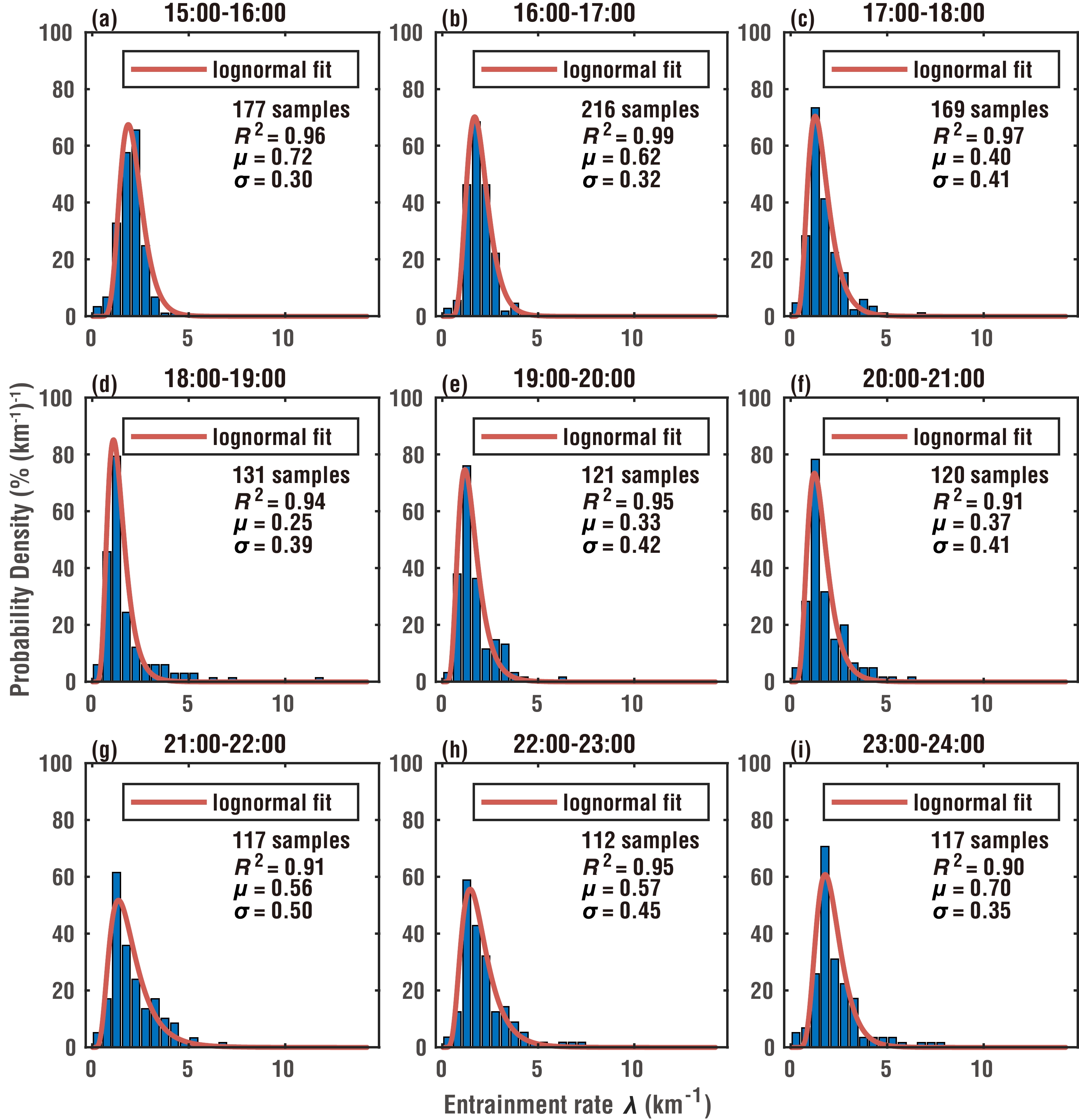
The PDF of cloud λ for all times and heights in Fig. 4 can present the characteristics of ensemble λ during the entire life cycle of the cumulus ensemble. It is also interesting to see whether there are differences in the PDFs of λ at different times, which could further improve the description of the entrainment process in the cumulus parameterization scheme. Figure 5 shows the PDF for all cloud λ for each hour from 1500 to 2400 UTC, along with the parameters of the log-normal fit and R². For the consistency of the time interval, the data of the two moments after 2400 UTC (13 samples) were not involved in the analysis. The R² in each time interval exceeded 0.90 (more than half attain 0.95), consistent with the results for all times and heights (Fig. 4). Furthermore, λ in each time interval was also described well by a log-normal distribution, further confirming the stochastic distribution of λ.

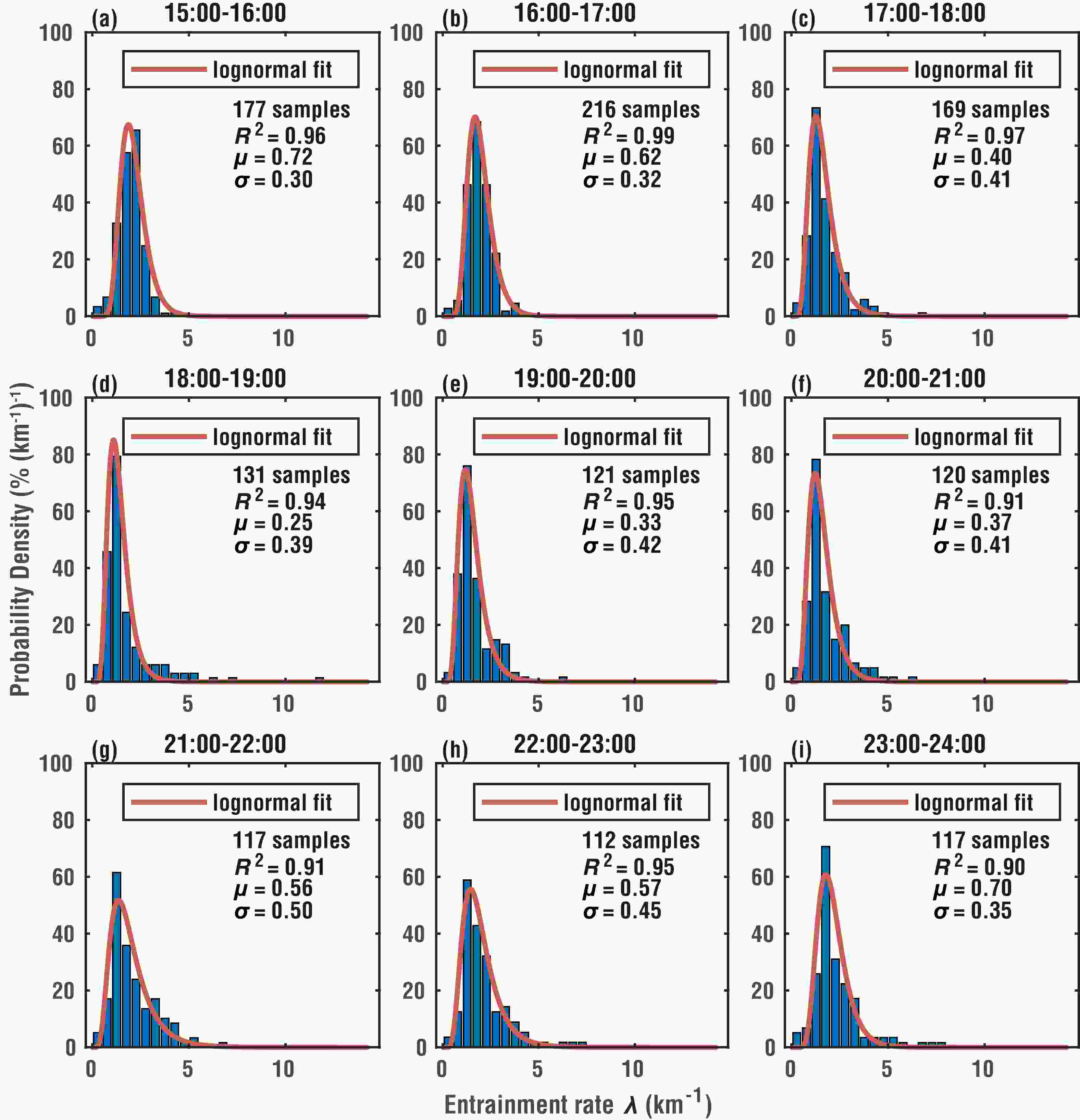
Figure 5.  Panels (a–i) represent the probability density function of the entrainment rate (λ) in hourly intervals from 1500 to 2400 UTC. The number of samples, coefficient of determination (R²), mean (μ), and standard deviation (σ) of ln(λ) for the log-normal fit (red line) in each time interval are provided.

Differences still existed between the distributions of λ for each time interval. The two parameters of the log-normal fit of λ were the mean (μ) and standard deviation (σ) of ln(λ). The μ initially decreased and then increased with time, and σ initially increased with time and decreased later. Thus, in the early stage of cloud ensemble development, λ was relatively large and the distribution was relatively concentrated. Over time, λ initially decreased and then increased, and its distribution gradually widened. At the end of the cloud life cycle, λ became relatively large and concentrated.

An accurate description of the PDF of λ in the model is of value for improving the simulation, which requires investigation of the factors affecting the PDF of λ. Previous studies have shown that w, B, and the environmental relative humidity (RH_e) are important factors, and these variables are often used to parameterize λ (Stirling and Stratton, 2012; de Rooy et al., 2013; Lu et al., 2016, 2018; Zhang et al., 2016; Bera and Prabha, 2019; Xu et al., 2021). Therefore, the effects of w, B, and RH_e on the PDF of λ are analyzed in this section. Note that w, B, and RH_e refer to the mean values of the cloud grid points as mentioned in section 2.

Similar to the analysis of the PDF of λ, PDFs were also calculated for w, B, and RH_e at each moment and fitted using a log-normal distribution. The hourly PDFs of w fitted well to a log-normal distribution (Fig. S2; in the ESM), and the results for the other variables were similar (figures not shown). This facilitated the analysis of the relationship between these variables and λ using the fitting parameters of the log-normal fit.

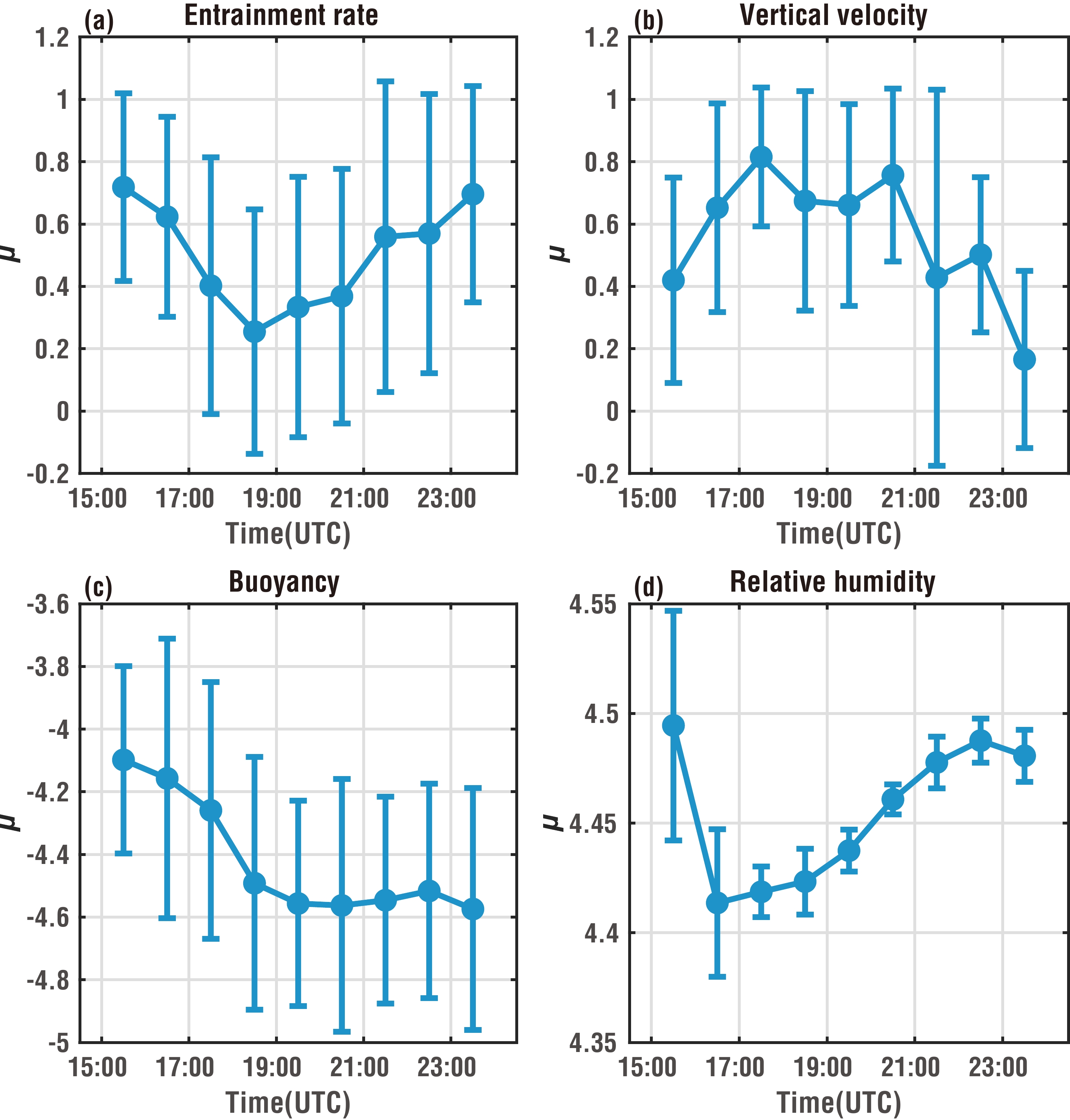
To determine the factors influencing the PDF of λ, the temporal variation of the parameters in the log-normal fit of the hourly PDF of λ, w, B, and RH_e was examined (Fig. 6). Consistent with the analysis in section 4.2.1, the mean value of λ initially decreased and then increased with time (Fig. 6a). In contrast, w initially increased and then decreased with time (Fig. 6b); thus establishing a negative correlation with λ. B generally decreased with time (Fig. 6c) and was not correlated with λ. The RH_e initially decreased and then increased with time (Fig. 6d) and was positively correlated with λ, although the timing of inflection points, from decreasing to increasing values, differed for λ and RH_e.

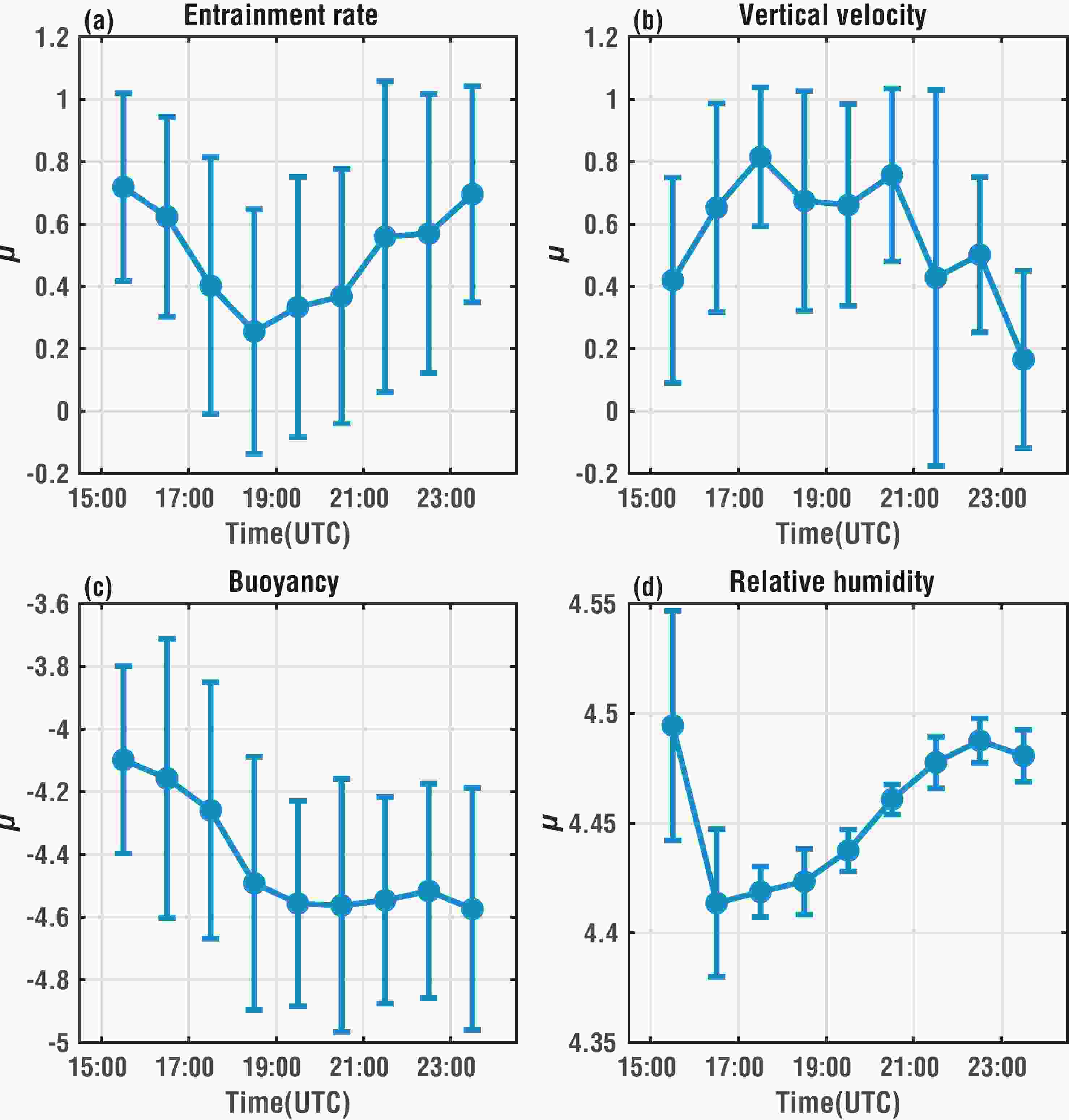
Figure 6.  Mean (μ) for the log-normal fit of the hourly probability density functions of (a) entrainment rate (λ), (b) vertical velocity (w), (c) buoyancy (B), and (d) environmental relative humidity (RH_e), as a function of time. Error bars represent the standard deviation (σ).

In summary, λ was negatively correlated with w, consistent with the results of many previous studies (de Rooy et al., 2013; Lu et al., 2016). Note that there was no significant correlation between λ and B, although previous studies have found a negative correlation between them (Lin, 1999; von Salzen and McFarlane, 2002). However, a lack of a significant correlation between λ and B was also found by Romps (2010). Gregory (2001) used B/w² to parameterize λ, a scheme that has been applied to climate models (Kim and Kang, 2012; Song and Zhang, 2018), showing that λ is positively correlated with B and negatively correlated with w. In previous studies, λ and B were found to be positively correlated, negatively correlated, or not correlated, suggesting that the effect of B on λ might be indirect. In contrast, w has a more direct effect on λ because when w is smaller, the cloud is allotted more time to mix with ambient air during ascent, which results in a larger λ (Neggers et al., 2002; Lu et al., 2016; Zhang et al., 2016; Xu et al., 2021). Lu et al. (2016) demonstrated that a larger λ reduces the temperature in the cloud when the ambient air and the cloud mix, thereby reducing B, while the decrease in B drives a decrease in w, which leads to an increase in λ. They also noted that w is the optimum choice when using a single variable to parameterize λ. Previous studies have shown that the relationship between λ and RH_e can be positive (Axelsen, 2005; Lu et al., 2018; Bera and Prabha, 2019; Stanfield et al., 2019; Zhu et al., 2021) or negative (Bechtold et al., 2008; Zhao et al., 2018b); and the results of this study tend to suggest a positive correlation. In conclusion, a relationship between w and λ is optimal.

Section 4.2 discussed variations in the PDF of λ over time. Because clouds and λ exhibit different distribution characteristics at different heights (Figs. 1–3), it is necessary to examine the variation of the PDF of λ with height. Similar to section 4.2.1, PDFs were calculated for λ per 200 m in the range 1000 m to 2600 m above sea level and fitted using a log-normal distribution. The PDFs of λ were well fitted in each height range (Fig. 7; R² exceeded 0.96, except for the PDF of 2400–2600 m), which further confirms that entrainment is a stochastic process. In the lower layer (Figs. 7a, b), μ was relatively large and σ was relatively small, indicating that λ of the lower layer was relatively large and the distribution was relatively concentrated. As height increased, μ initially decreased and then increased, whereas σ increased gradually. Correspondingly, λ initially decreased and then increased with height, and the distribution became increasingly dispersed. Interestingly, the PDF was narrow at lower altitudes (mainly due to the identical properties of most cloud ensembles in the formation stage) and became wider as height increased (mainly due to cloud variability brought forth by the coexistence of cloud ensembles in multiple stages). The PDFs of λ at all heights in an LES, as presented by Dawe and Austin (2013), showed that λ strongly followed a log-normal distribution and the mean PDF of all individual cumulus cloud λ was consistent with the cloud ensemble λ. Furthermore, λ initially decreased with height and then remained unchanged, and increased at high levels, similar to the vertical distribution obtained in this study.

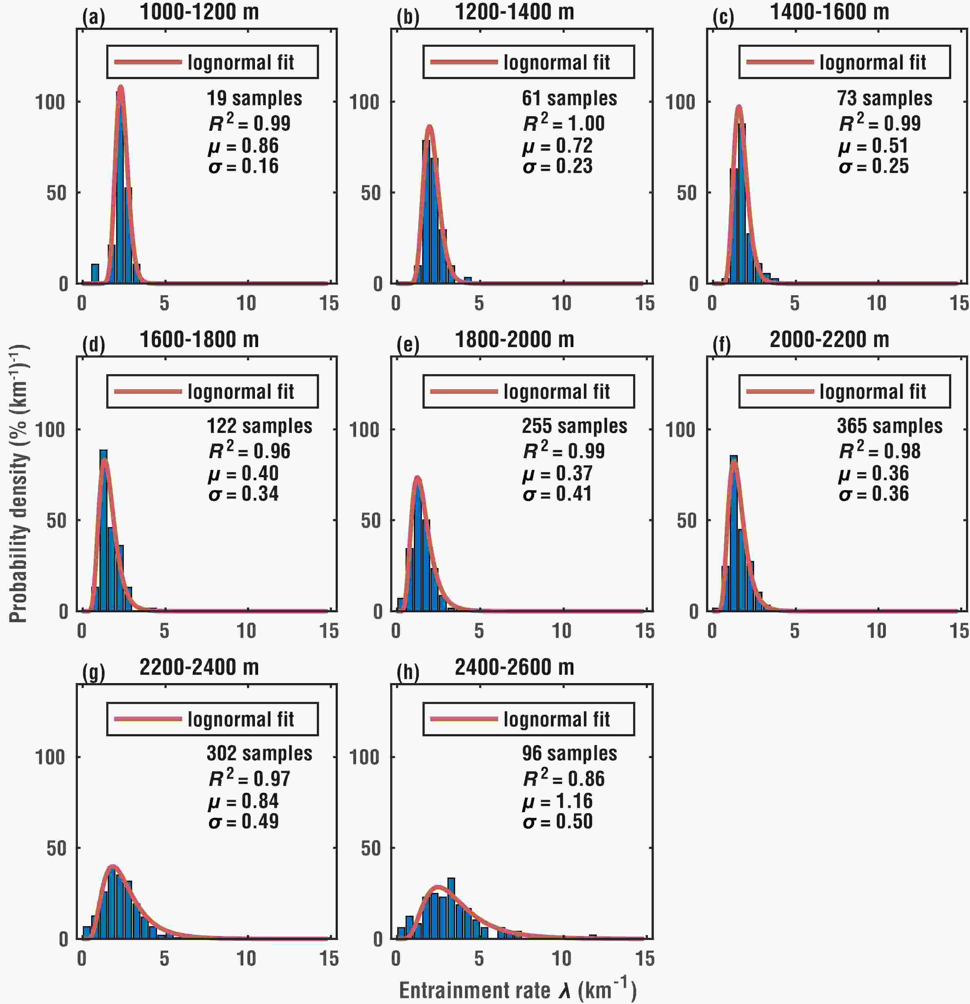
Figure 7.  Panels (a–h) represent the probability density function of the entrainment rate (λ), in 200-m increments, over the range of 1000 to 2600 m. The number of samples, coefficient of determination (R²), mean (μ), and standard deviation (σ) of ln(λ) of the log-normal fit (red line) in each 200 m are provided.

The factors influencing the PDF of λ were analyzed in section 4.2.2. In this section, we discuss whether these same conclusions apply to the PDFs of λ at different heights. Similar to section 4.2.2, log-normal distributions were fitted to the PDFs of w, B, and RH_e for each 200-m range. The PDFs of w within each 200-m range were well fitted by a log-normal distribution (Fig. S3; in the ESM) and the results for the other variables were similar (figures not shown). Figure 8 shows variations in the fitting parameters of the PDFs of λ and its influencing factors, as a function of height, to analyze the relationship between λ and influencing factors at different heights.

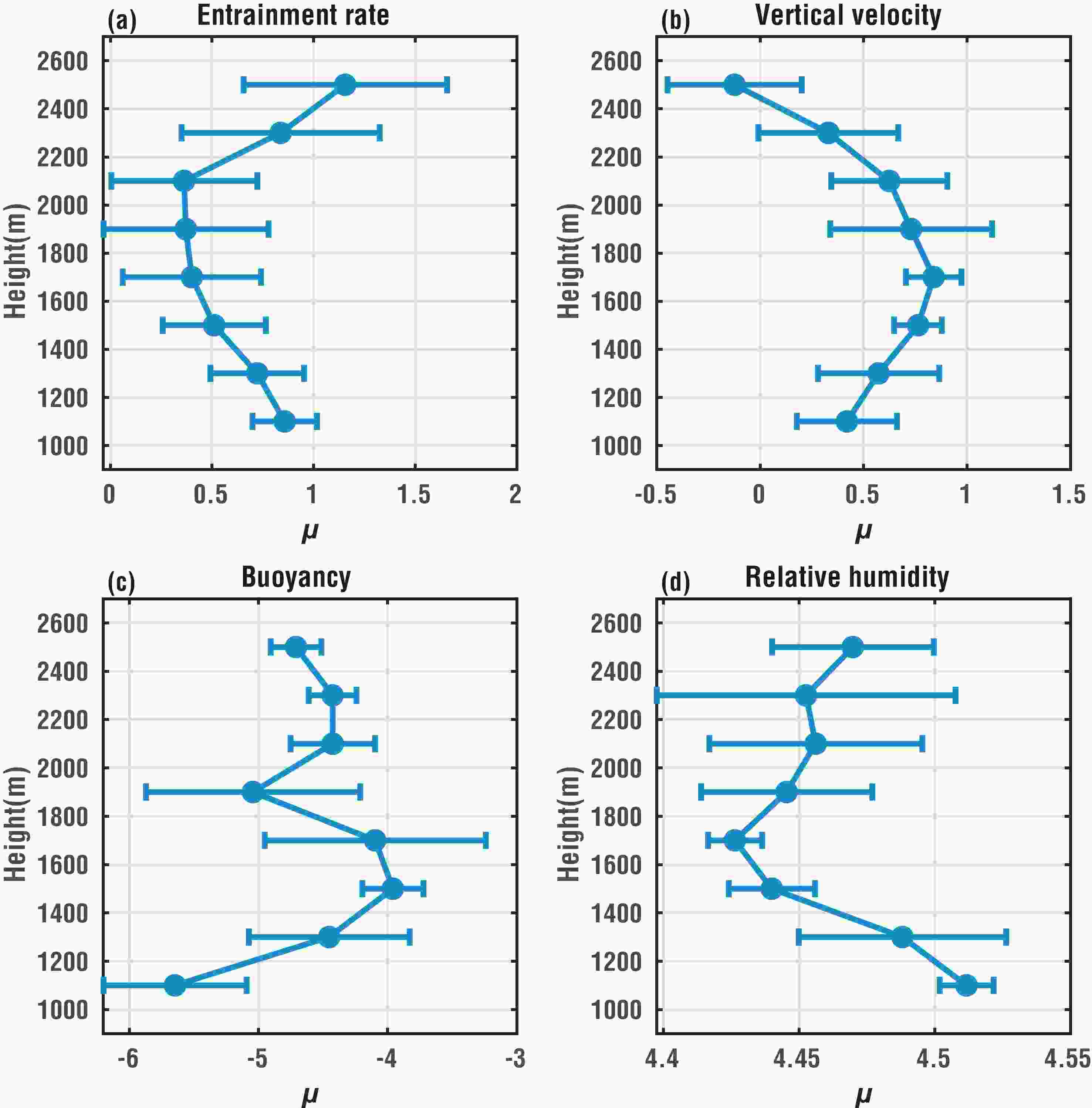
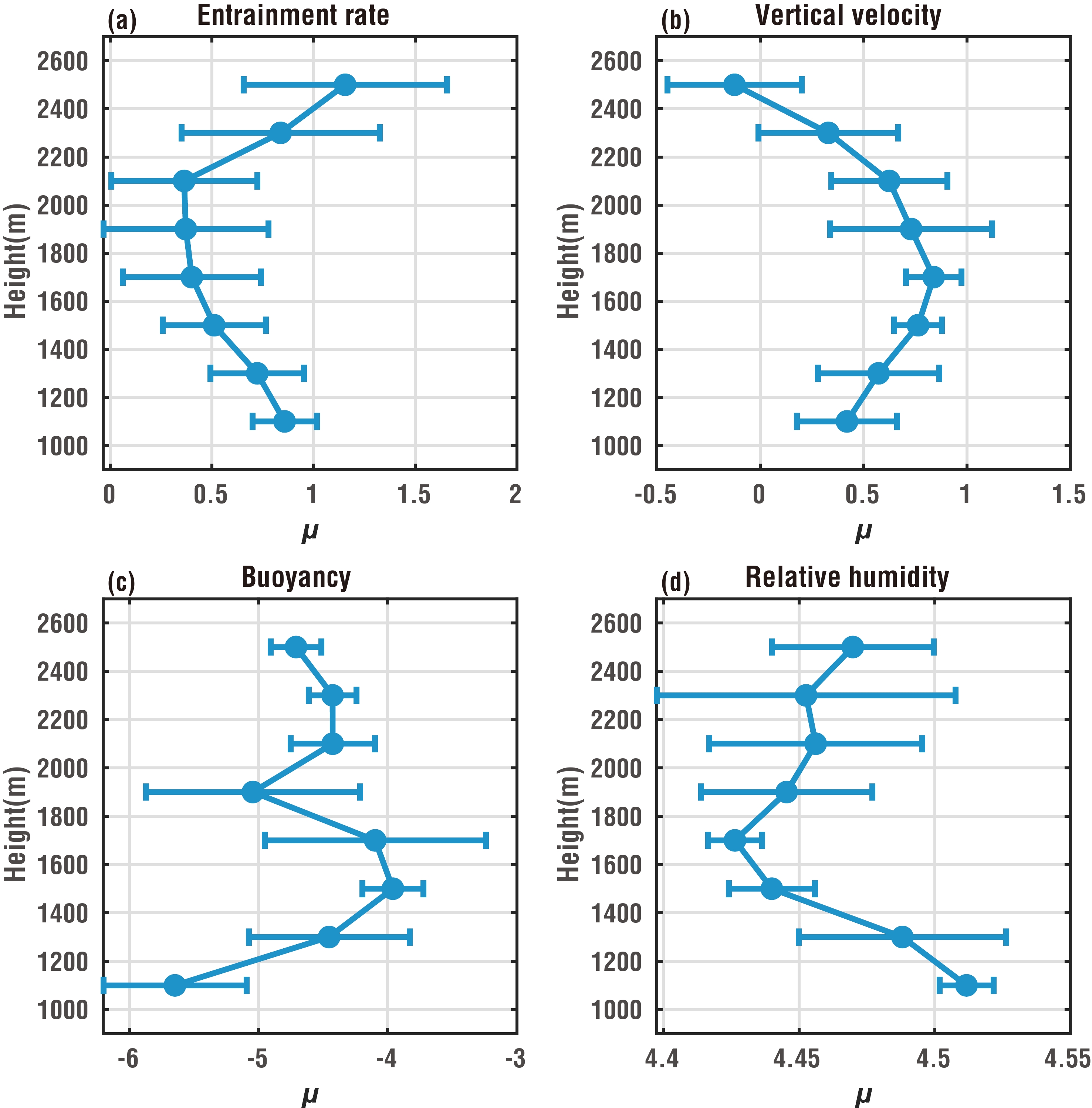
Figure 8.  Mean (μ) of the log-normal fit of the probability density functions of (a) entrainment rate (λ), (b) vertical velocity (w), (c) buoyancy (B), and (d) environmental relative humidity (RH_e) in each 200-m layer as a function of height. Error bars represent the standard deviation (σ).

The mean value of λ initially decreased and then increased with height (Fig. 8). In contrast, w initially increased and then decreased with increasing height, and λ and w were negatively correlated. B initially increased and then decreased with increasing height and was negatively correlated with λ. However, there was a small value in 1800–2000 m, which was inconsistent with the vertical change in λ. The vertical profiles of λ and B have a better correspondence compared with the time-series plots of λ and B in Fig. 6. The RH_e initially decreased and then increased with height, consistent with the vertical distribution of λ; the corresponding relationship between these two variables was also better than that apparent in Fig. 6. In conclusion, the relationship between λ and each influencing factor at different heights is similar to that at different times (section 4.2.2). Furthermore, similar to Fig. 8, the vertical distributions of the fitting parameters for the PDFs of λ and its influencing factors were plotted for the three stages of the cloud ensembles (Fig. S1; in the ESM). Comparisons of the results for the three stages and that for all times show similar vertical distributions, and w has the best relationship with λ in the three stages. Combining the results of different heights and times, the relationship between λ and w is the strongest.

The entrainment rate (λ) is an important physical variable in cumulus parameterization schemes. The accurate calculation of λ from observations or high-resolution simulations is key to improving λ parameterization. The probability density function (PDF) of λ can be very useful for treating cumulus convection in models. Therefore, this study applied a large-eddy simulation of cumulus clouds to calculate λ based on the improved bulk-plume method and analyzed the spatial and temporal distributions of λ, including variations of the PDF of λ with time and height and its influencing factors. The main conclusions are as follows:

First, an improved method for calculating λ was developed and its accuracy was validated. The improved method, which solves the conservation equations of two variables simultaneously, is an improvement over the traditional bulk-plume method. The calculated λ, based on the improved method, numerically falls within the range of λ values calculated by the traditional bulk-plume method using two different conserved variables, indicating the reliability of the improved method.

Second, the spatial and temporal distributions of λ were examined. During the entire life cycle of the cumulus ensemble, λ initially decreased and then increased; that is, λ in the formation and dissipation stages was larger than that during the maintenance stage. In terms of its vertical distribution, λ generally exhibited an initial decline and then an increase with increasing height. Regardless of its overall characteristics or variations with time and height, the PDF of λ was well fitted by a log-normal distribution, demonstrating that it is reasonable to treat λ as a stochastic process in numerical simulations. This study provides the PDF of λ to facilitate the randomization of the entrainment process in models.

Finally, the main factors affecting the spatial and temporal distributions of λ were determined. For the variation of PDF with time and height, λ was negatively correlated with the vertical velocity (w) and positively correlated with environmental relative humidity (RH_e), consistent with previous studies. There is a poor correlation between λ and buoyancy (B) with respect to time, but the relationship between λ and B was generally negative as a function of vertical height. Overall, the relationship between λ and w was the strongest. These findings offer insight and a new point of reference for handling stochastic entrainment processes in a cumulus parameterization scheme (i.e., assuming a log-normal PDF).

Two points are noteworthy. First, in future parameterizations of λ, it is recommended that w is used as the primary factor. In addition, the influences of RH_e, B, and other factors cannot be ignored. It is necessary to comprehensively analyze the effects of these factors on λ by combining more observations and high-resolution simulations so that the model convection scheme can describe entrainment more accurately. Moreover, as pointed out by Böing et al. (2012), the detrainment rate is even more important than λ in determining the vertical distribution of convective cloud mass. Thus, accurately obtaining the detrainment rate in cumulus clouds is fairly important to improve cumulus parameterization schemes.

Second, the improved method proposed here can be applied to aircraft observations. Because it is difficult to obtain multiple observations of the same shallow cumulus cloud by aircraft, there is usually only one horizontal penetration for each cumulus cloud. For aircraft observations, the detection height of the aircraft and the height of the cloud base can be taken as two height levels to obtain a large number of observational λ values of individual cumulus clouds. To increase the accuracy of the measurement of λ in future aircraft observations, it is highly recommended to measure multiple layers of the same cumulus cloud and the interval between each layer should be as small as feasibly possible. Additionally, the improved method can also be applied to remote sensing data such as enhanced ground-based radar observations, which can obtain the vertical distribution of λ in a large horizontal range.

Acknowledgements. The authors would like to thank Jianfeng GU at Nanjing University for the helpful discussions. This research is supported by the National Natural Science Foundation of China (Grant Nos. 42175099, 42027804, 42075073) and the Innovative Project of Postgraduates in Jiangsu Province in 2023 (Grant No. KYCX23_1319). Shi LUO is supported by the National Natural Science Foundation of China (Grant No. 42205080), the Natural Science Foundation of Sichuan (Grant No. 2023YFS0442), and the Research Fund of Civil Aviation Flight University of China (Grant No. J2022-037). This research is also supported by the National Key Scientific and Technological Infrastructure project “Earth System Science Numerical Simulator Facility” (EarthLab). The numerical calculations in this paper were conducted on the supercomputing system in the Supercomputing Center of Nanjing University of Information Science & Technology.

Data availability The large-scale forcing data used in this study can be downloaded from the Atmospheric Radiation Measurement (ARM) user facility (https://doi.org/10.5439/1647300 (Tao and Xie, 2004); https://doi.org/10.5439/1647174 (Tao and Xie, 2012)). LASSO data can be downloaded from https://doi.org/10.5439/1342961 (Gustafson et al., 2017).

Electronic supplementary material: Supplementary material is available in the online version of this article at https://doi.org/10.1007/s00376-023-2357-6.