The Influence of Arctic Sea Ice Concentration Perturbations on Subseasonal Predictions of North Atlantic Oscillation Events

The North Atlantic Oscillation is the seesaw-like phenomenon in sea-level pressure (SLP) between the Icelandic Low and Azores High in the North Atlantic sector (Walker and Bliss, 1932). It is one of the most dominant low-frequency atmospheric variabilities in the mid-to-high latitudes of the Northern Hemisphere during boreal winter. The NAO not only influences weather in the region but also greatly impacts the global climate (Hurrell, 1995; Diao et al., 2015). Both the Icelandic Low and the Azores High weaken during the negative phase of the NAO (NAO–), causing cold in Europe and North America, while both atmospheric centers strengthen and induce warm winters there during its positive phase (NAO+) (Thompson et al., 2000; Hurrell and Deser, 2010).

The NAO has trended toward its negative phase during past decades, which is considered to be related to Arctic sea ice reduction (Francis et al., 2009; Vihma, 2014; Cohen et al., 2020). It has been reported that the Arctic sea ice concentration (SIC) reduction in autumn could modulate the planetary waves of the Barents-Kara Seas (BKS) and favor an NAO– response in winter (Jaiser et al., 2012, 2013). However, Arctic SIC anomalies in different sectors could trigger various NAO responses (Screen, 2017; McKenna et al., 2018). By diagnosing the reanalysis data, it is found that the NAO tends to favor its negative phase in its response to SIC reduction in the BKS, while the positive phase often accompanies SIC decline in the Canadian Archipelago (Luo et al., 2016). Moreover, SIC variability in the Pacific can lead to various NAO responses by triggering Rossby waves there (Yamamoto et al., 2006; Mesquita et al., 2011).

However, the intrinsic timescale is approximately 20 days for the NAO life cycle (Feldstein, 2003). On this timescale, NAO events are usually related to extreme weather events in Eurasia. For example, the Middle East was affected by an extreme heavy snow event in December 2013, whose primary cause was believed to be a decaying NAO+ event (Luo et al., 2015). The essence of such a relationship inspires us to investigate NAO events on subseasonal timescales.

An NAO event can be treated as a nonlinear initial value problem on the synoptic timescale and the initial condition plays the dominant role in NAO evolution (Benedict et al., 2004; Franzke et al., 2004; Luo et al., 2007, 2008). Perturbations in both the troposphere and even the stratosphere are crucial for NAO evolution (Luo et al., 2008; Nie et al., 2019). With the help of a quasi-geostrophic model, Jiang et al. (2013) investigated the optimal precursors (OPR) which trigger the onset of NAO events 5–8 days in advance. Moreover, they investigated the optimally growing initial errors (OGIE) in NAO onset predictions and discussed the relationship between the OPR and OGIE (Dai et al., 2016). After that, they further discussed the target observations to improve the prediction skills of NAO event onsets (Dai et al., 2019).

In addition to synoptic timescales, much attention has been dedicated to subseasonal forecasts over the last decade (Vitart et al., 2017). Their work reveals that skillful forecasts are available with lead times longer than two weeks (Buizza and Leutbecher, 2015). For example, with a lead time of 2–4 weeks, the ECMWF can skillfully forecast the extreme cold frequency in boreal winter (Xiang et al., 2019; 2020). For certain strong and long-lasting cold events in East Asia, skillful forecasts could be made two weeks in advance or earlier (Dai and Mu, 2020; Dai et al., 2021a). Apart from synoptic timescales, both the atmospheric initial condition and boundary conditions e.g., sea surface temperature (SST) and SIC, are crucial for atmospheric evolution on subseasonal timescales (Liu et al., 2017; Wang et al., 2018), especially for large-scale atmospheric circulations like the NAO (Mariotti et al., 2020).

It is found that sea ice anomalies could trigger a baroclinic atmospheric response with surface heat flux modification and such atmospheric responses can reach an equivalent barotropic structure in two months (Deser et al., 2007). Moreover, utilizing the Integrated Forecasting System from ECMWF, Semmler et al. (2016) investigated the influence of sudden Arctic sea ice thinning on atmospheric circulations by introducing a 10°C warming in sea ice surface temperature. They found that the atmosphere has a baroclinic response in the first several days due to the boundary layer process and reaches a quasi-equilibrium state in two months. After that, Dai et al. (2021b) discussed the impact of sudden Arctic sea ice thinning on NAO events. Their results reveal that NAO events have different responses to sudden Arctic sea ice thinning due to various NAO circulation patterns. The above results show that Arctic sea ice is an important boundary condition for atmospheric evolution on subseasonal timescales.

However, large uncertainties exist in Arctic sea ice datasets, which greatly impact subseasonal atmospheric circulations (Dai and Mu, 2020). Rather than integrating the numerical model with various boundary conditions, the conditional nonlinear optimal perturbation (CNOP) approach is efficient in revealing the largest influence of Arctic SIC on an NAO event. The CNOP approach was first proposed to solve for the initial uncertainty in ENSO prediction (Mu et al., 2003) and was further developed to solve for the uncertainty in model parameters (Mu et al., 2010), model tendencies (Duan and Zhou, 2013), and boundary conditions (Wang and Mu, 2015). The CNOP approach is widely utilized in investigating atmospheric and oceanic problems, as summarized in Wang et al. (2020). Recently, Ma et al. (2022) investigated the role of Arctic sea ice anomalies in the subseasonal forecasts of Ural blocking events with CNOP approaches. Their results indicate that SIC in the Greenland, Barents, and Okhotsk seas is crucial for the prediction of Ural blocking on subseasonal timescales.

Due to the relationships between NAO events and Eurasian extreme weather, we attempt to investigate the following questions. (1) What kind of Arctic sea ice perturbations could exert the greatest influence on NAO event predictions on subseasonal timescales? (2) What is the physical mechanism by which Arctic sea ice perturbations affect NAO event prediction? Understanding their solutions may help us conceptualize the role of Arctic SIC in NAO formation. Additionally, these solutions can provide scientific support in the Arctic SIC target observations and the ensemble perturbation generations, which can further improve the NAO event predictions.

The remainder of this paper is organized as follows. In section 2, the data and methods are described in detail. In section 3, the response time of NAO events to Arctic SIC perturbations is determined by sensitivity numerical experiments. The optimal Arctic SIC perturbations for NAO+ and NAO– events are explored in sections 4 and 5, respectively. Finally, the conclusion and discussion are presented in section 6.

Daily atmospheric and oceanic data with a 1.0° × 1.0° resolution from the ERA-Interim reanalysis are used in this investigation (Dee et al., 2011). The atmospheric variables include sea level pressure (SLP), surface air temperature, 300-hPa geopotential height (Z300) and 500-hPa geopotential height (Z500), and the 300-hPa and 500-hPa zonal winds in winter (December, January, and February), spanning the period from 1981/82 to 2000/01. The daily oceanic variables include SST and SIC spanning January 1982 to December 2001. The SIC data are derived from the Special Sensor Microwave Imager Sounder based on a smooth combination of Bootstrap and Bristol algorithms (Comiso, 1986; Dee et al., 2011). These daily oceanic variables are used as the boundary conditions for the numerical model, noting that the period 1982–2001 is consistent with the default forcing settings in the numerical model.

The Community Atmospheric Model, version 4 (CAM4) with prescribed SST and SIC is utilized in this investigation (Neale et al., 2013). The atmospheric model has 26 vertical levels with a top at approximately 3.5 hPa, and the horizontal resolution is approximately 0.9° × 1.25°. The model settings are the same as those in Dai et al. (2021b). Briefly, the calendar means of the ERA-Interim daily SST and SIC ranging from January 1982 to December 2001 are used as the prescribed model boundary condition, while the CO₂ concentration is set to 367 ppmv. These are consistent with the other default settings in CAM4. Moreover, the sea ice thickness is uniformly set to 2 meters in the Arctic and 1 meter in the Antarctic. The numerical model has been run for 31 years with the first year of model data being discarded as the model spin-up period. The remaining 30 years of model data are adopted for analysis. Compared with the reanalysis data, CAM4 has a good representation of the atmospheric circulation during wintertime, which has been evaluated in Dai et al. (2021b).

Similar to that in Dai et al. (2021b), the NAO index (NAOI) is used to describe the NAO phase and intensity. The NAOI is defined as the scaled projection of the daily SLP anomaly on the typical positive NAO anomaly mode. The formula can be expressed as:

where $ {\mathrm{S}\mathrm{L}\mathrm{P}}_{\mathrm{N}\mathrm{A}\mathrm{O}} $ represents the typical positive NAO mode in the SLP field, which is derived from the first empirical orthogonal function of the daily SLP anomaly in the North Atlantic sector (approximately 20°–80°N, 90°W–40°E). $ {\mathrm{S}\mathrm{L}\mathrm{P}}_{\mathrm{d}} $ is the daily SLP anomaly relative to the climatology. The angle brackets denote the Euclidean inner product.

Similar to the NAO event definition in Dai et al. (2021b), an NAO+ (NAO–) event is identified when the daily NAOI is larger than 1.0 (smaller than –1.0) for five or more consecutive days. The first day with NAOI larger than 1.0 (smaller than –1.0) is defined as the NAO+ (NAO–) onset day (marked as lag 0 day). Similarly, 15, 10, and 5 days before NAO onset are marked as lag–15, lag–10, and lag–5 days, respectively, while the day corresponding to 5 days after onset is marked as lag+5 day. According to the above criteria, 22 NAO+ and 22 NAO– events are recognized from the 30-year CAM4 simulation, showing a similar frequency to the 13 NAO+ and 14 NAO– events in the 20-year ERA-Interim reanalysis. The NAO events in the CAM4 simulation are not expected to coincide with those in the reanalysis. However, the compositions show that CAM4 describes the evolution of such NAO events well and thus can be utilized for further investigation [see Figs. 4 and 5 in (Dai et al., 2021b)].

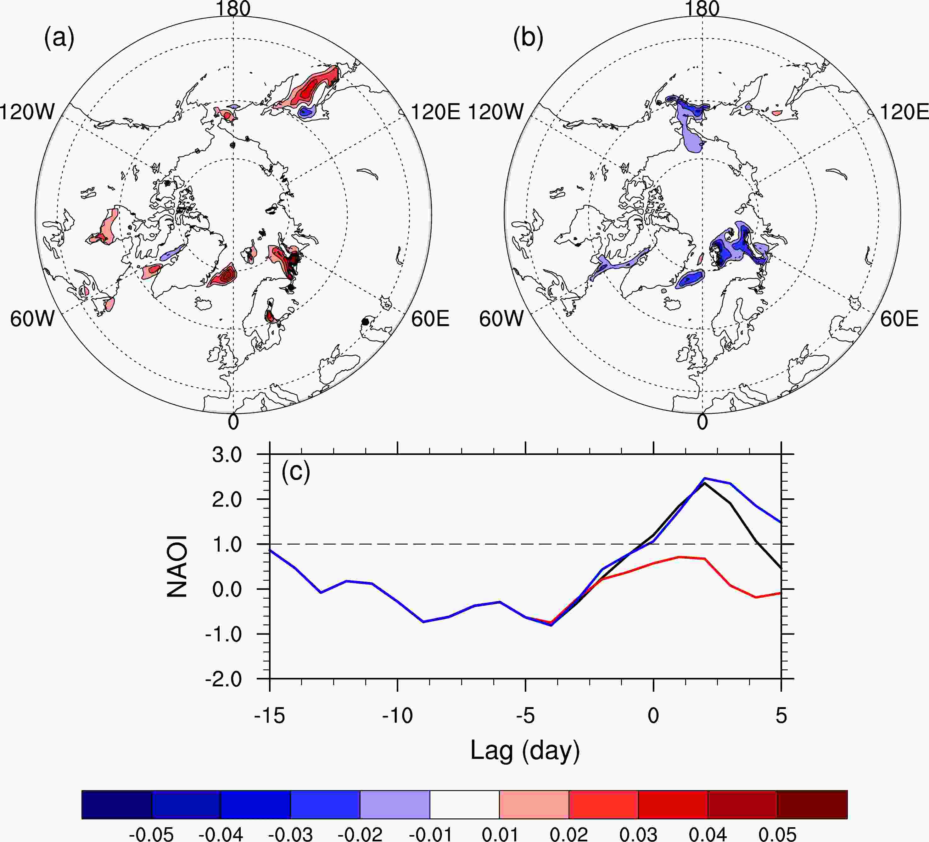
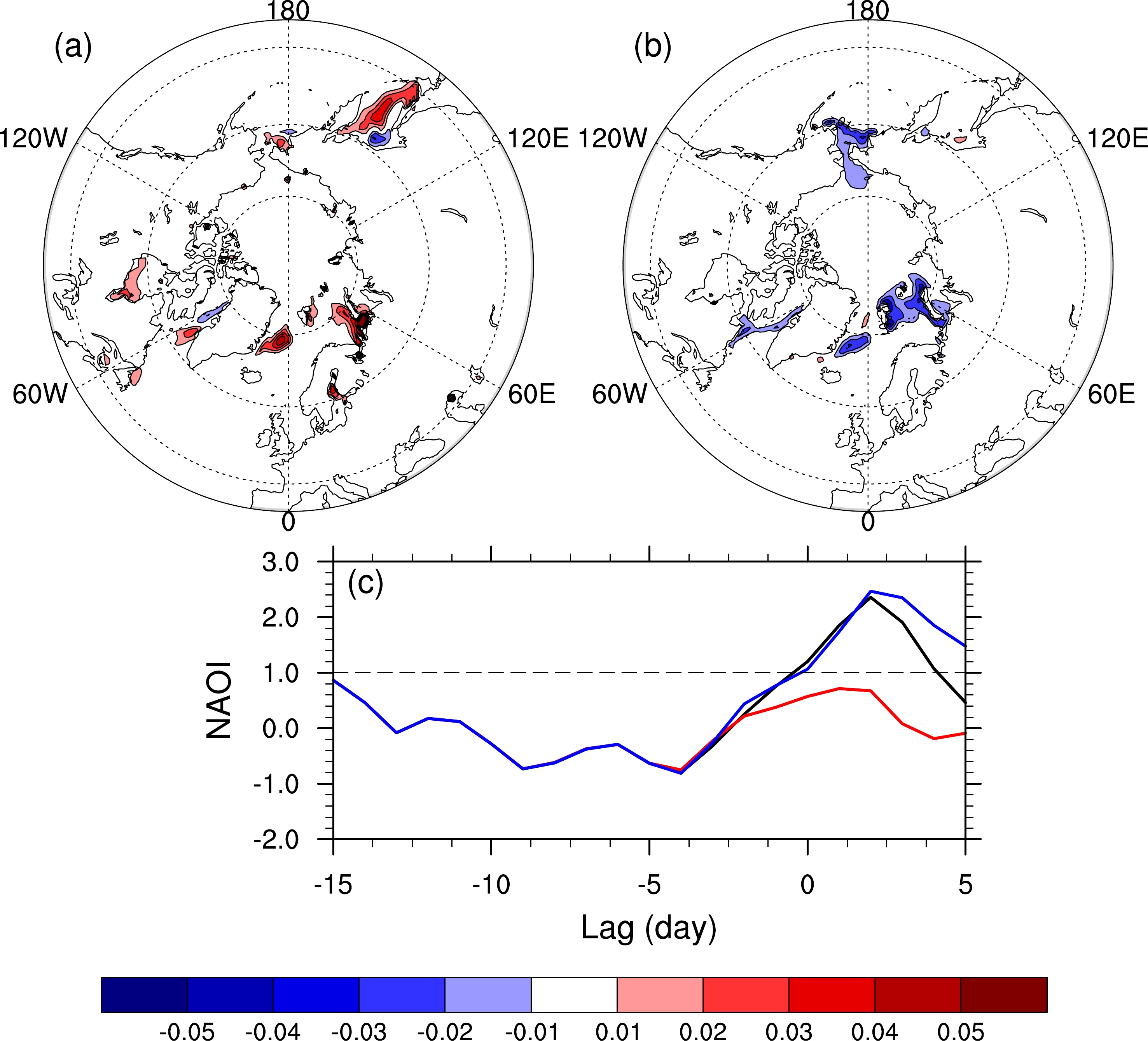
Figure 4.  (a) Type-1 and (b) type-2 optimal SIC perturbations for the first simulated NAO+ event prediction. Panel (c) shows the NAOI evolution derived in the reference state (black), type-1 optimal SIC perturbation (red), and type-2 optimal SIC perturbation (blue).

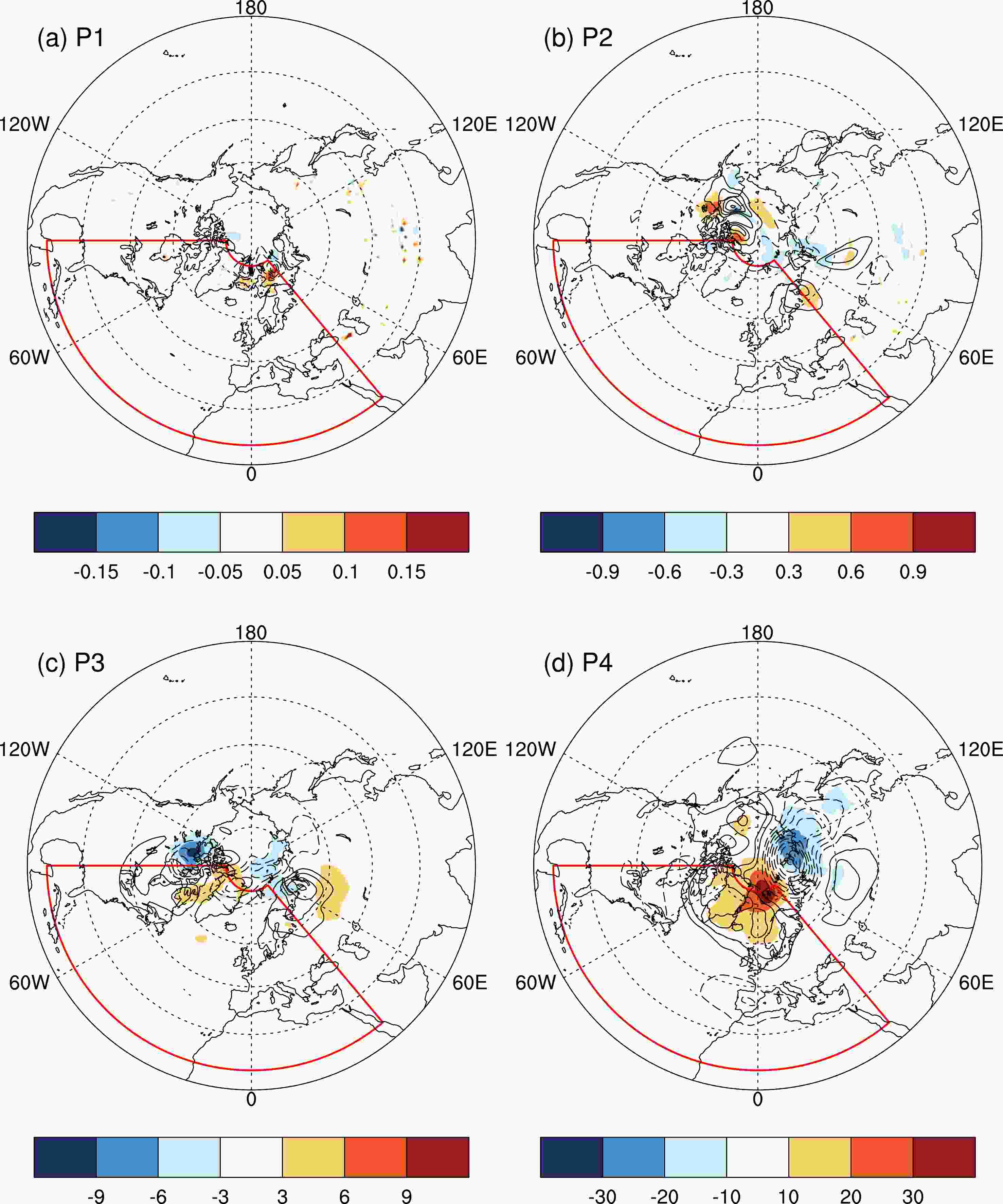
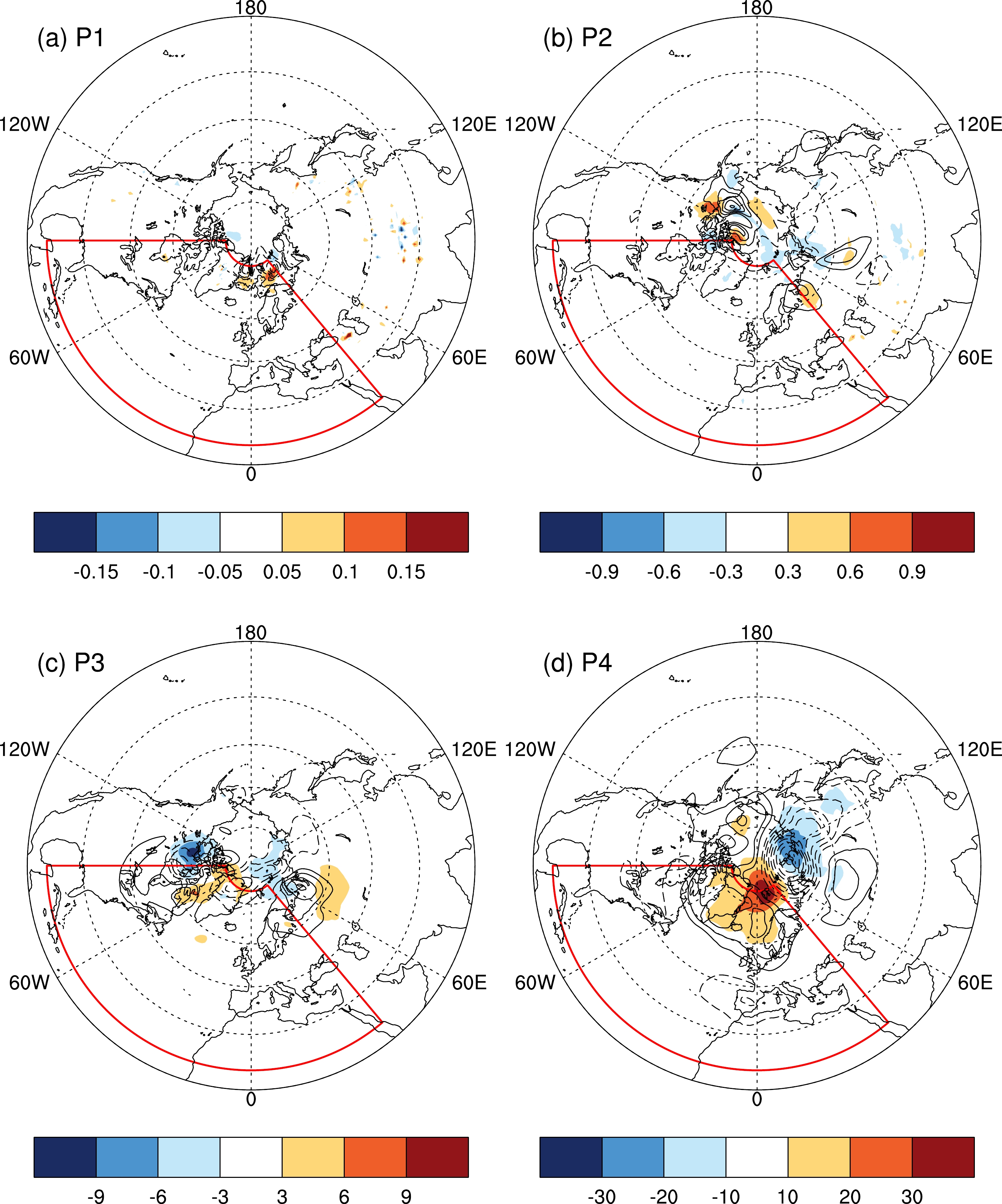
Figure 5.  SLP (shading, units: hPa) and Z500 response (contour, units: gpm) to type-1 optimal SIC perturbations during the (a) 1st pentad (CI = 0.2 gpm), (b) 2nd pentad (CI = 2.0 gpm), (c) 3rd pentad (CI = 20 gpm) and (d) 4th pentad (CI = 40 gpm) for the first simulated NAO+ event. The red box in each panel indicates the North Atlantic sector (20°–80°N, 90°W–40°E).

To investigate the influence of Arctic SIC on NAO event predictions on subseasonal timescales, the CNOP for boundary uncertainty (CNOP-B, Wang and Mu, 2015) is utilized since the Arctic SIC is treated as the boundary condition in the CAM4 model. In this investigation, CNOP-B represents the specific Arctic SIC perturbation that causes the largest uncertainty of the NAO evolution under a given physical constraint. Since the NAOI can measure the phase and intensity of an NAO event, the corresponding objective function is defined as the NAOI difference induced by the Arctic SIC perturbations at the optimization time, which can be expressed as:

where B₀ is the boundary condition in the reference state and b₀ is the Arctic SIC perturbation. In particular, b₀ denotes the Arctic SIC perturbation coverage from 40° to 90°N and is time-independent, indicating that the SIC perturbation is unchanged during the integration period. Therefore, $ {\mathrm{N}\mathrm{A}\mathrm{O}\mathrm{I}}_{{B}_{0}+{b}_{0}}^{T} $ and $ {\mathrm{N}\mathrm{A}\mathrm{O}\mathrm{I}}_{{B}_{0}}^{T} $ correspond to the NAOI derived from the model integrations with and without Arctic SIC perturbations at the optimization time T, respectively. Moreover, $\left\|{b}_{0}\right\|\leqslant \delta$ is the constraint of the Arctic SIC perturbation, which can be expressed as:

where i and j represent the location of each grid point and $ {\phi }_{i,j} $ is the corresponding latitude. The constraint $ \delta $ is 10^–4 in this investigation, which indicates the average SIC perturbation on each sea ice grid point is approximately 0.01. This constraint is comparable to the uncertainty in SIC products (Singarayer et al., 2005; Dai and Mu, 2020). It should be noted that there are some SIC perturbations greater than 0.01 and some less than 0.01 since the SIC perturbations are spatially inhomogeneous. The solution to Eq. (2) is represented by $ {b}_{0}^{*} $ which represents the specific Arctic SIC perturbation that has the largest influence on an NAO event. It should also be noted that the optimal SIC perturbations are case-dependent, which are influenced by the atmospheric initial conditions. That is, optimal SIC perturbations for different NAO events vary.

To solve the nonlinear optimization problem [i.e., Eq. (2)], a particle swarm optimization (PSO) intelligent algorithm is utilized in this investigation due to the inaccessible adjoint model in CAM4. The PSO algorithm was inspired by the predation behavior of birds and is effective in solving the nonlinear optimization problem without adjoint models (Kennedy and Eberhart, 1995; Shi and Eberhart, 1999). The specific algorithm has been detailed and illustrated by Mu et al. (2015). However, the rotated empirical orthogonal function is utilized for the Arctic SIC dimension reduction due to the high dimensionality of Arctic SIC perturbations, which is similar to that of Ma et al. (2022). The first 20 leading patterns are used to represent the Arctic SIC variability, which explains more than 80% of the observed daily Arctic SIC variability in boreal winter. The PSO method is considered to have obtained a solution if the objective function value does not increase in the following 15 iterations. We adopted 20 particles to solve the nonlinear optimization problem and the optimal Arctic SIC perturbations are usually obtained in 30 iterations.

This investigation explores the influences of Arctic SIC on NAO-event formations on subseasonal timescales. As mentioned in a previous study, the case of successive NAO events or phase transition events is more complicated, and their evolutionary mechanism may be distinct from that in traditional NAO formations (Luo et al., 2014). Therefore, we only consider the traditional NAO event in this investigation, which requires the NAOI to be between –1.0 and 1.0 within 15 days before its onset. According to this criterion, there are five NAO+ and five NAO– events in the 30-year CAM4 simulation. These NAO events also have strong intensities.

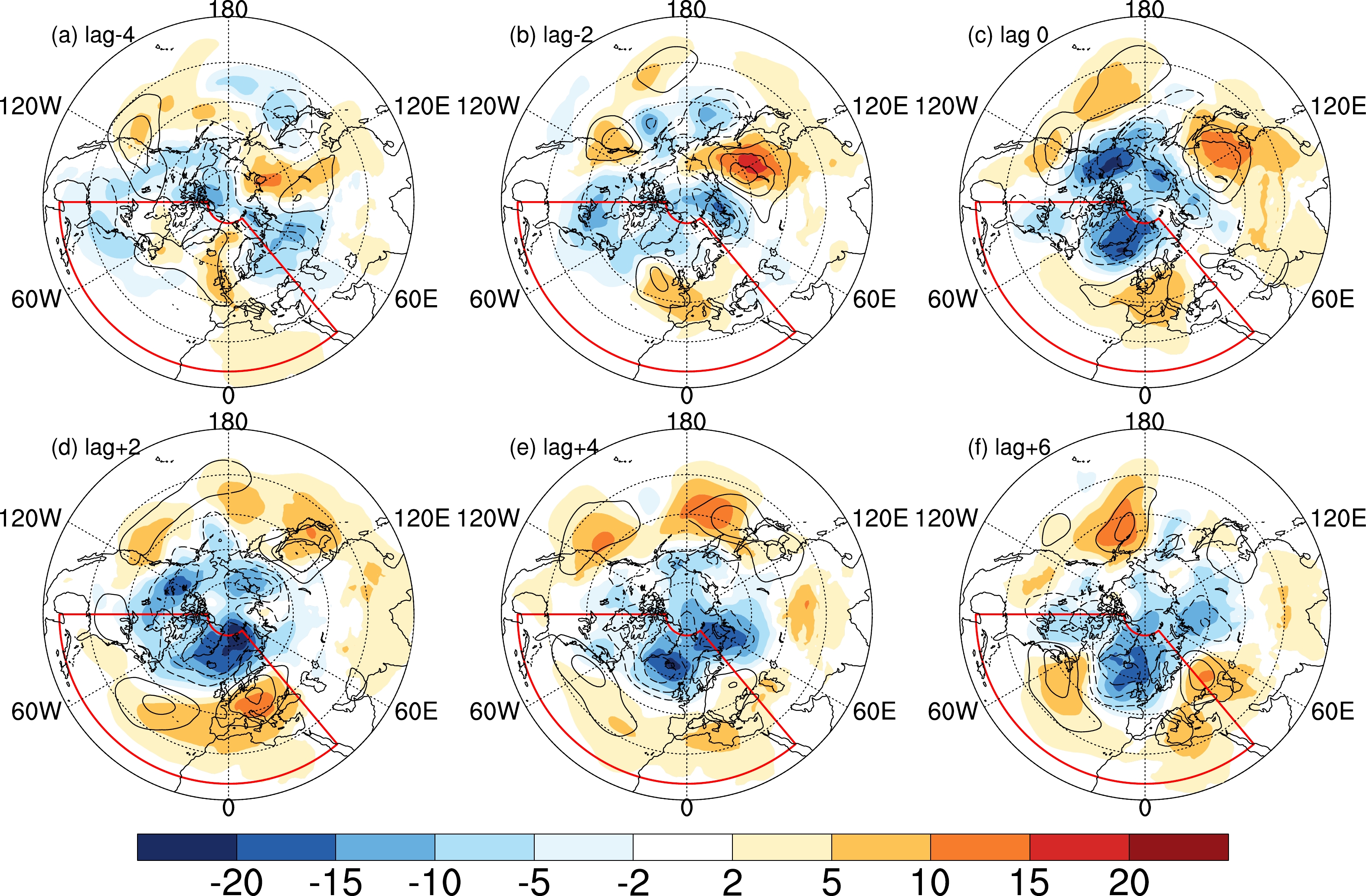
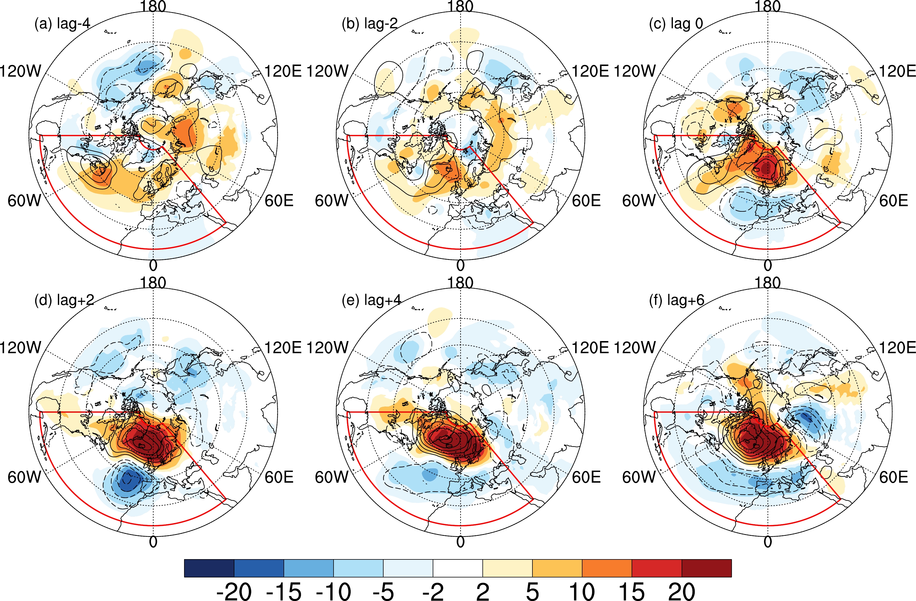
The composite SLP and Z500 anomalies of these five NAO+ events are shown in Fig. 1. It shows that the Rossby waves propagate from the North Pacific and evolve to a negative-over-positive structure in the North Atlantic. Regarding the NAO– events, their evolution shows an in situ developmental feature (Fig. 2). The local development in NAO– events is consistent with that in observations (Benedict et al., 2004). The evolutionary behaviors of each NAO event are shown in Figs. S1 and S2 in the electronic supplementary materials (ESM). The evolutionary behaviors of the composite simulated NAO events are similar to those in observation, indicating that CAM4 has a good description of the NAO evolutions. Therefore, these cases are used to further explore the Arctic SIC influence on NAO event predictions.

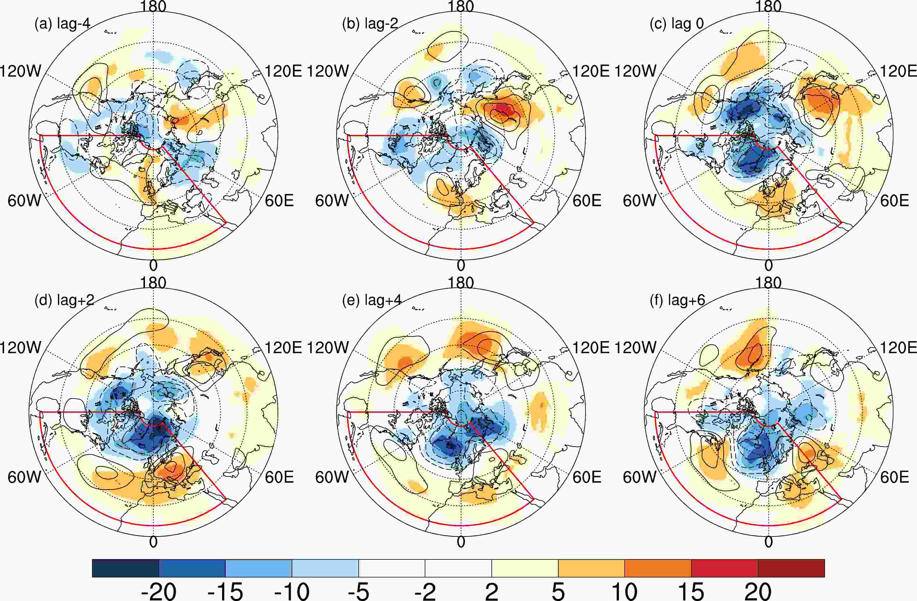
Figure 1.  Composite SLP anomaly (shading, units: hPa) and Z500 anomaly (contour, units: gpm) during the NAO+ events at (a) lag–4, (b) lag–2, (c) lag 0, (d) lag+2, (e) lag+4 and (f) lag+6 day in CAM4 simulation. Lag 0 denotes the NAO+ onset day. Solid and dashed lines represent positive and negative anomalies, respectively. The contour interval (CI) is 40 gpm and the zero line is omitted. The red box in each panel indicates the North Atlantic sector (20°–80°N, 90°W–40°E).

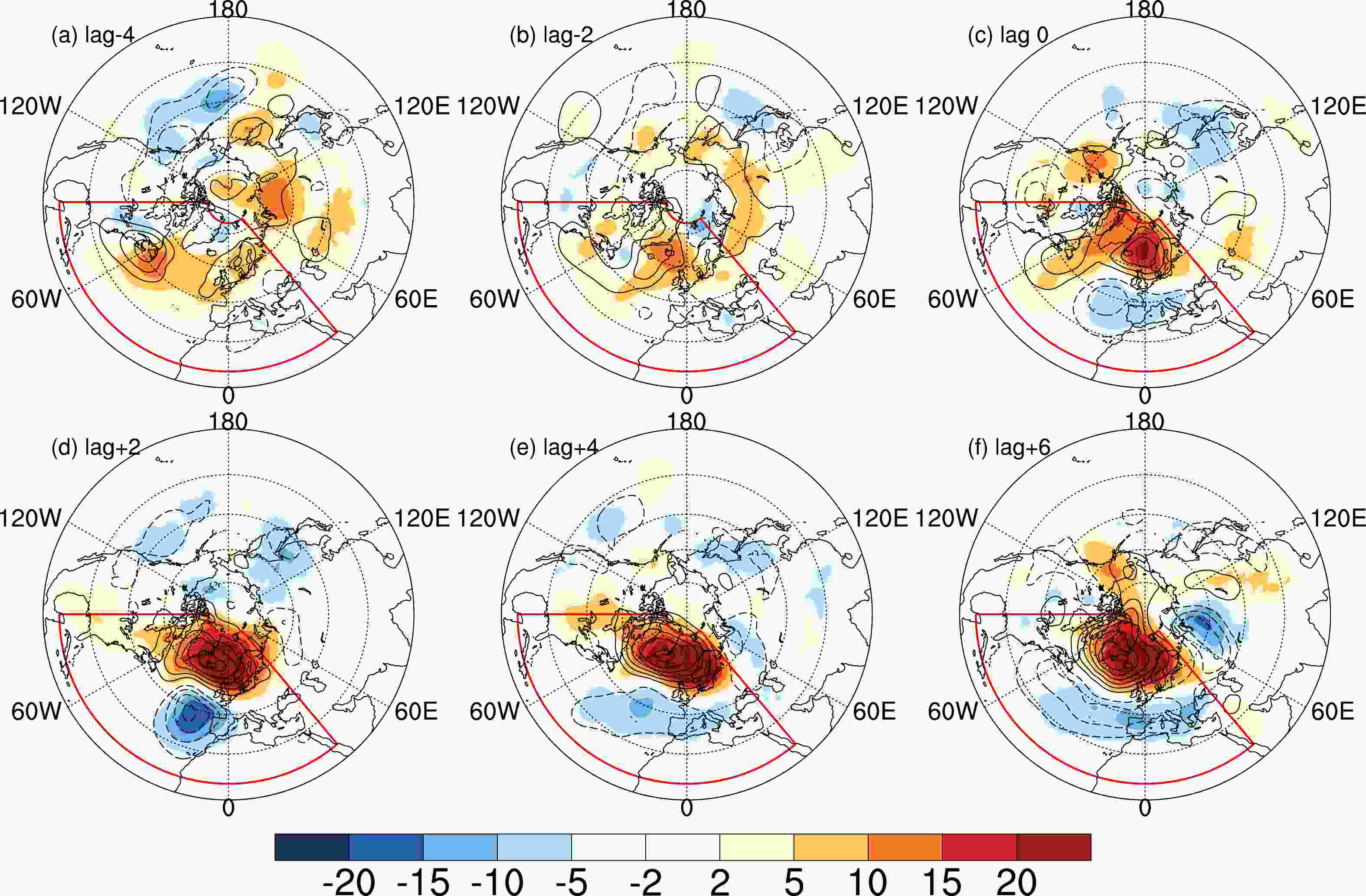
Figure 2.  Same as in Fig. 1, but for the five NAO– events in the CAM4 simulation.

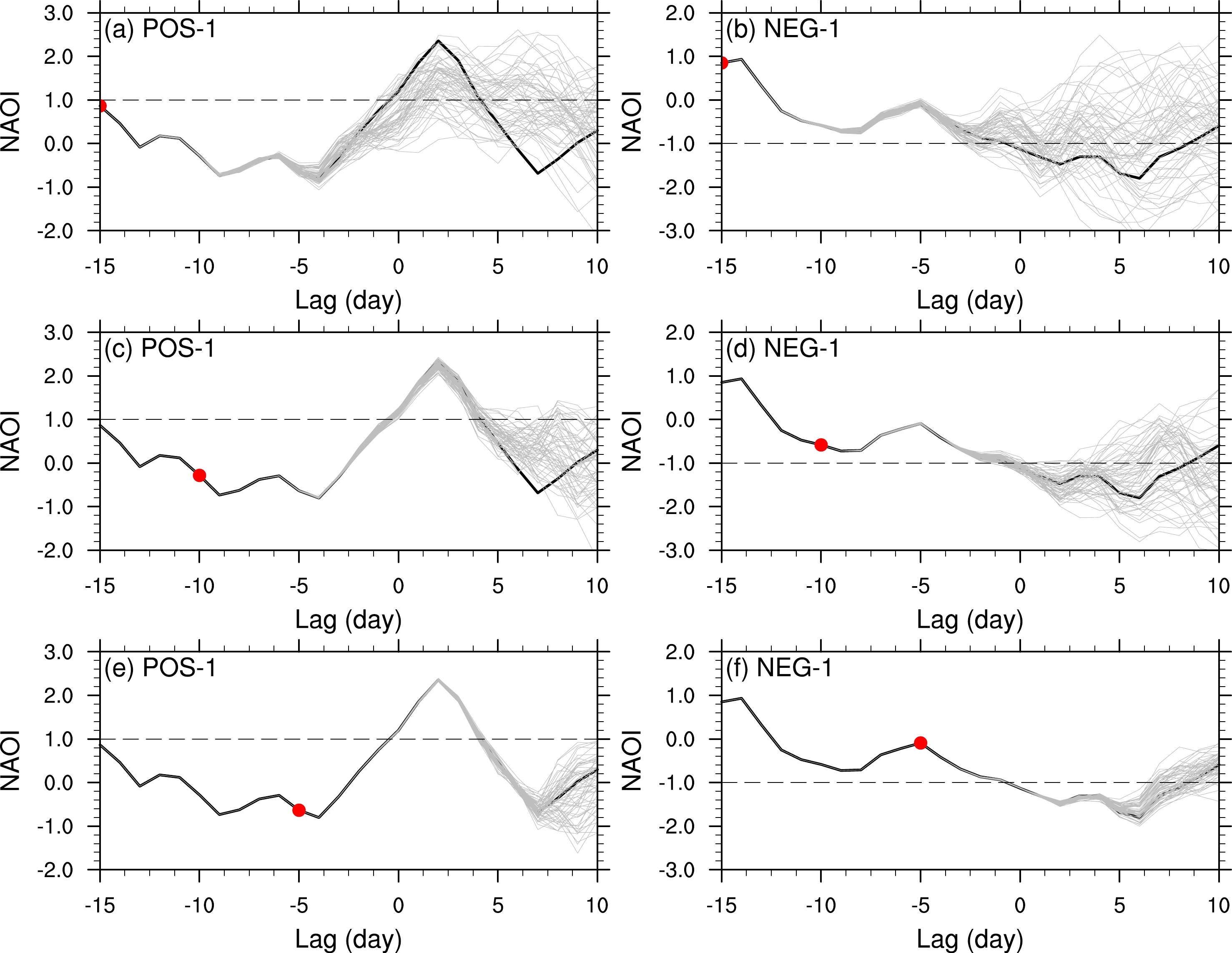
Similar to those in Dai et al. (2021b), some sensitivity experiments are conducted to determine the response time of NAO events to SIC perturbations. Specifically, 60 monthly Arctic SIC anomalies in winter (December, January, and February) ranging from 1981/82 to 2000/01 are obtained from ERA-Interim. These 60 SIC perturbations have been superimposed on the boundary conditions from 15 days (lag–15 day), 10 days (lag–10 day), and 5 days (lag–5 day) before the NAO onset respectively, and last to 15 days after the NAO onset. It should be noted that these observed Arctic SIC perturbations are added at the start of each integration, and unchanged during the whole integration period. The numerical model is run for 30 days to explore the Arctic SIC influence on NAO events. As shown in Fig. 3 and Figs. S3−S4 in the ESM, the NAO shows obvious responses from the lag–5 day with the Arctic SIC perturbed 15 days in advance of the NAO onset. The Arctic SIC perturbations are likely to cause uncertainties in the NAO onset (lag 0 day), as well as the NAO development and decay periods (Figs. 3a, b). With a start time 10 days in advance of the NAO onset (lag–10 day), there is little influence on the NAO onset (lag 0 day) but there are many impacts on the NAO development and decay periods (Figs. 3c, d). Regarding the Arctic SIC perturbed from 5 days ahead of the NAO onset (lag–5 day), there is almost no obvious impact on the NAO onset or development periods, but there are some uncertainties during their decay periods (Figs. 3e, f). That is, the entire NAO life cycle would be influenced if the Arctic SIC has been perturbed 15 days before its onset, indicating that Arctic SIC is a predictability source for subseasonal NAO event predictions. This result is similar to the effect of the sudden thinning of Arctic sea ice (Dai et al., 2021b). Therefore, the Arctic SIC perturbation 15 days in advance of the NAO onset is adopted to explore the Arctic SIC influence on NAO event predictions.

Figure 3.  NAOI responses to Arctic SIC perturbations with different lead times. The left panels correspond to Arctic SIC perturbations at (a) 15, (c) 10, and (e) 5 days before the first simulated NAO+ event onset where the x-axis is time, and the y-axis is the NAOI. In each panel, the thick black line indicates the NAOI with no Arctic SIC perturbation, while 60 gray lines correspond to the NAOI derived with different Arctic SIC perturbations. The red dots represent the lead time for superimposing Arctic SIC perturbations, while lag 0 corresponds to the NAO onset day. Panels (b), (d), and (f) are similar to (a), (c), and (e), but for the first simulated NAO– event.

As mentioned previously, the SIC perturbations have been superimposed on the basic boundary conditions 15 days in advance of the NAO onset (lag–15) and last until the end of model integration. Since we are going to investigate the influence of Arctic SIC perturbations on NAO event predictions on subseasonal timescales, the pentad average has been adopted to remove the high frequency impacts. Consequently, lag–15 to lag–11, lag–10 to lag–6, lag–5 to lag–1, and lag 0 to lag+4 days correspond to pentads 1, 2, 3, and 4, respectively, and pentad 4 is the formation stage for NAO event, including the onset day of NAO event and following four days. Therefore, the corresponding objective function evolves to the difference between the 4th pentad-average NAOI, which can be expressed as:

where $ {\mathrm{N}\mathrm{A}\mathrm{O}\mathrm{I}}_{{B}_{0}+{b}_{0}}^{P4} $ and $ {\mathrm{N}\mathrm{A}\mathrm{O}\mathrm{I}}_{{B}_{0}}^{P4} $ are the pentad-average NAOI derived from the numerical model integration with and without boundary perturbations during the formation stage (the 4th pentad), respectively. As the objective function (Eq. 4) is in an absolute value form, two solutions may exist. One solution corresponds to $ {\mathrm{N}\mathrm{A}\mathrm{O}\mathrm{I}}_{{B}_{0}+{b}_{0}}^{P4} $larger than $ {\mathrm{N}\mathrm{A}\mathrm{O}\mathrm{I}}_{{B}_{0}}^{P4} $, while another solution corresponds to $ {\mathrm{N}\mathrm{A}\mathrm{O}\mathrm{I}}_{{B}_{0}+{b}_{0}}^{P4} $ smaller than $ {\mathrm{N}\mathrm{A}\mathrm{O}\mathrm{I}}_{{B}_{0}}^{P4} $.

Taking the five NAO+ events as the reference states, the corresponding nonlinear optimal problems have been solved. The first NAO+ event is used as an example to illustrate the influences of optimal Arctic SIC perturbations on NAO+ event predictions. For the first NAO+ event, two types of optimal SIC perturbations have been obtained by solving the corresponding nonlinear optimal problem. Type-1 optimal SIC perturbations exhibit positive SIC anomalies mainly in the Greenland Sea, Barents Sea, and Okhotsk Sea (Fig. 4a), while type-2 optimal SIC perturbations show negative SIC perturbations in the Bering Sea, Greenland Sea, and Barents Sea (Fig. 4b). Superimposing these two types of optimal SIC perturbations on the reference boundary conditions and allowing them to persist for the whole integration period, the corresponding NAOI evolutions are shown in Fig. 4c. These two types of SIC perturbations have nearly the same evolutionary NAOI as the reference state in the first two pentads (lag–15 to lag–6 days). However, they have distinct influences on NAO events in pentads 3 and 4 (lag–5 to lag 4 days). Type-1 optimal SIC perturbations lead to a smaller NAOI evolution in pentads 3 and 4 compared with the reference state (red line in Fig. 4c), underestimating the NAO+ event. Moreover, the NAOI derived with type-1 optimal SIC perturbations is smaller than 1.0 during pentad 4. Therefore, the NAO+ event no longer exists due to type-1 SIC perturbations. However, for type-2 optimal SIC perturbations, the corresponding NAOI has a small difference from the reference state during pentad 3 but exhibits a larger NAOI evolution during pentad 4 (blue line in Fig. 4c), which overpredicts the NAO+ event. The influence of type-1 optimal Arctic SIC perturbations is larger than that of type-2 perturbations. Moreover, both types of SIC perturbations exert a much greater influence on NAO event predictions compared with the random SIC perturbations under the same constraint (not shown). This suggests that only perturbations in specific patterns are likely to trigger great impacts on NAO predictions, while randomly structured perturbations have little influence on them.

Figure 5 shows the SLP and Z500 responses induced by type-1 optimal SIC perturbations. During pentad 1, there is a positive SLP anomaly and negative geopotential height anomaly at 500 hPa in the Barents Sea (Fig. 5a). Soon thereafter, the SLP and Z500 anomalies spread in the Arctic (north of 60°N) during pentad 2. However, the SLP anomalies are less than 1 hPa in amplitude and almost outside of the North Atlantic sector, which did not have an obvious influence on the NAO+ event (Fig. 5b). For pentad 3, there are some positive SLP anomalies over Baffin Bay, as well as some negative SLP anomalies over the Canadian Arctic Archipelago (Fig. 5c). Therefore, a somewhat negative NAOI response is shown in pentad 3. However, the 4th pentad shows a positive SLP response over Greenland and Barents Seas and a negative SLP response over the East Siberian Sea. It also shows a positive geopotential height response over the North Atlantic sector and a negative 500 hPa geopotential height response over East Siberia. The responses in SLP and geopotential height near 500 hPa exhibit a quasi-barotropic structure (Fig. 5d). Thus, the positive response in the North Atlantic sector weakens the north center of the NAO+ dipole and causes the NAO+ event to cease to exist. However, the SLP and Z500 responses induced by type-2 optimal SIC perturbations have nearly opposite evolutionary behaviors compared to those triggered by type-1 optimal SIC perturbations but with a much smaller amplitude (Fig. S5).

Both types of optimal SIC perturbations have notable influences on NAO+ event predictions in all four pentads, and type-1 SIC perturbations even result in the NAO+ event being too weak to exist. Therefore, type-1 SIC perturbations are taken as an example to illustrate the physical mechanism by which Arctic SIC perturbations influence NAO+ event prediction in the four pentads.

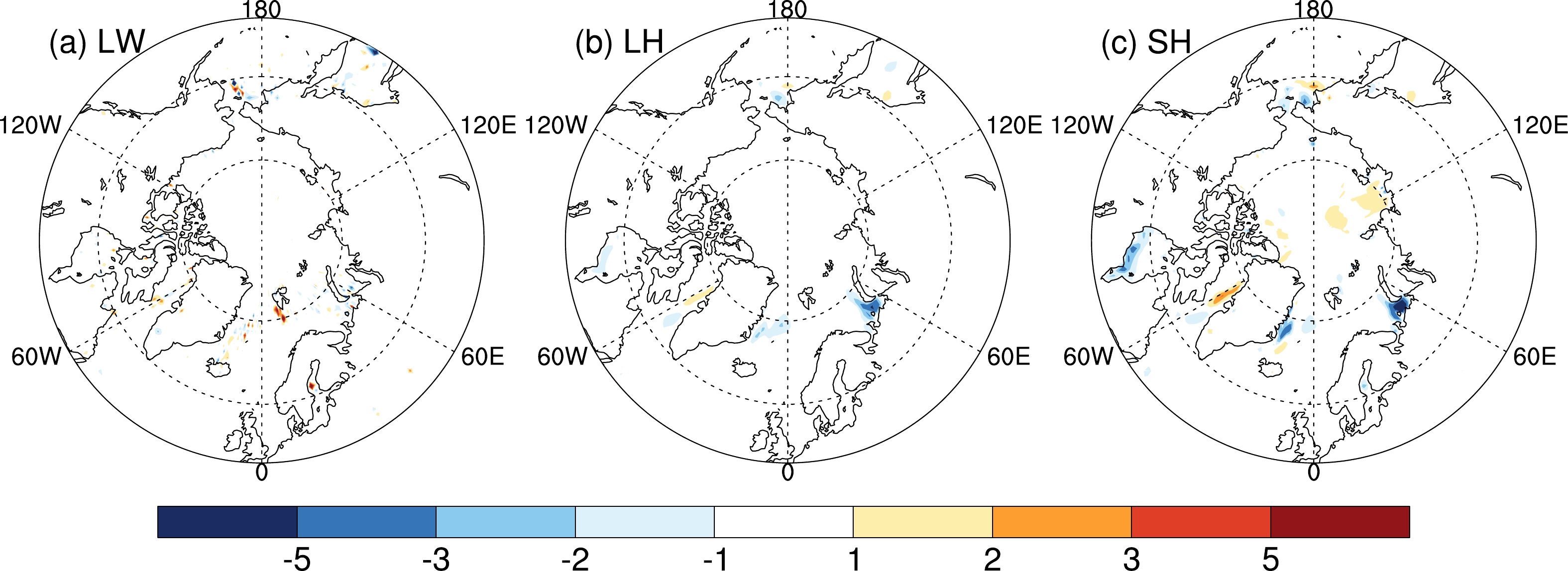
As the Arctic SIC is perturbed, the corresponding heat fluxes between the sea ice and air change. Figure 6 shows the longwave radiation, latent heat flux, and sensible heat flux responses to the type-1 optimal SIC perturbations on the first day. Shortwave radiation has little influence on NAO events during boreal winter and is not discussed here. As shown in Figs. 6b and c, there are some negative latent heat flux and sensible heat flux responses in Greenland and Barents Seas. These turbulent heat flux response patterns correspond to positive SIC anomalies, which prevent heat transport from the ocean to the air. The response of longwave radiation is smaller than that of turbulent heat flux (Fig. 6a).

Figure 6.  (a) Longwave radiation, (b) latent heat flux, and (c) sensible heat flux responses (units: W m^–2) to type-1 SIC perturbations on the first day.

As the heat flux between the sea ice and air changes, the air temperature in the low troposphere causes a consequential response. Figure 7 shows the 700-hPa temperature response for the four pentads. Triggered by type-1 optimal SIC perturbations, there is some cooling over the Barents and Greenland seas during the 1^st pentad (Fig. 7a). The cooling is consistent with the SIC perturbations and the heat flux responses, suggesting that the 700-hPa temperature responds via the diabatic process. For pentad 2, the temperature response in the North Atlantic sector is small, but there is a significant temperature response around the Canadian Archipelago (Fig. 7b). However, for the 3rd pentad, the 700-hPa temperature shows a cooling response in northern Greenland but somewhat of a warming response over the Canadian Archipelago and Barents-Kara Seas. The 4th pentad shows a warming response in Greenland at 700 hPa, which corresponds to the nearly barotropic geopotential height response there. Moreover, there is a negative-over-positive temperature response in northern Siberia and the Barents-Kara Seas, which agrees with the geopotential height response there (Fig. 5d).

Figure 7.  700-hPa temperature response (units: K) to type-1 SIC perturbations during the (a) 1st pentad, (b) 2nd pentad, (c) 3rd pentad, and (d) 4th pentad. The red box in each panel indicates the North Atlantic sector (20°–80°N, 90°W–40°E).

The heat budget equation in pressure coordinates is utilized to reveal the temperature evolution induced by the optimal SIC perturbations (Hoskins et al., 1989), which can be formulated as:

where T, $ \mathbf{V} $, and $ \omega $ correspond to the temperature, horizontal and vertical velocity, while p, $ \theta , $ and Q correspond to the pressure, potential temperature, and diabatic heating rate, respectively. Moreover, $ {p}_{0} $, R and c_p are constants, representing the standard atmospheric pressure (i.e., 1000 hPa), the dry-air specific gas constant, and the specific heat capacity. According to Eq. (5), the local temperature variability is controlled by three terms: the horizontal temperature advection ($ -\mathbf{V}\cdot \nabla T $), vertical temperature convection $[-{\left( {p}/{{p}_{0}}\right)}^{\frac{R}{{C}_{p}}} \omega {\partial \theta }/{\partial p}$], and diabatic heating process (${Q}/{{C}_{p}}$).

Figure 8 shows that both the horizontal and vertical temperature advection play important roles in the 700-hPa temperature response in these two pentads. However, the diabatic process is less important in these two pentads than in dynamic terms. That is, the 700-hPa temperature response is mainly influenced by diabatic processes in the 1st pentad but controlled by dynamic processes (horizontal advection and vertical convection) later. Thus, it is not surprising that temperature responses cover the Northern Hemisphere. Furthermore, there is a baroclinic response in Z500 due to the geopotential height increases in the warming sectors and the geopotential height decline in the cooling sectors. The perturbed Z500 could further influence the atmospheric circulation via dynamic processes afterward.

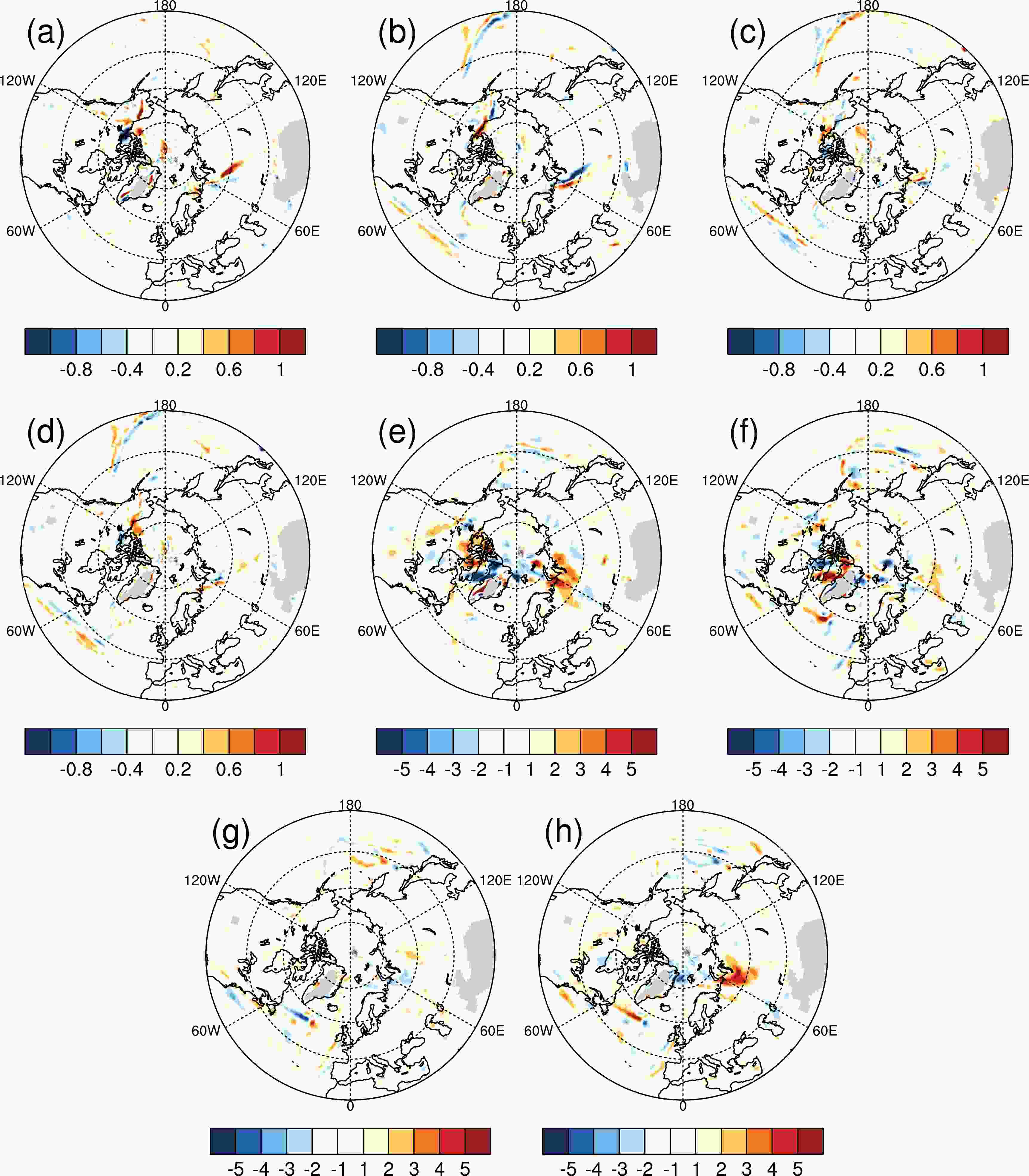
Figure 8.  Decomposition of the 700-hPa temperature response during pentads 2 and 3 (units: K d^–1). Panel (a) is the horizontal advection term, (b) is the vertical convection term, (c) is for diabatic heating processes, and (d) is the dynamic term (i.e., the sum of horizontal and vertical advection) in pentad 2. Panels (e)–(h) are similar to (a)–(d) but for pentad 3.

As mentioned previously, the response in SLP (Z500) is less than 1 hPa (10 gpm) during pentads 1−2, which has little influence on NAOI. However, for pentads 3−4, there are large responses in SLP and Z500, which obviously influence the NAOI evolution. Therefore, the response in SLP and Z500 during pentads 3−4 are further investigated. For the Z500 evolution, its behavior could be explained with the quasi-geostrophic potential vorticity equation (Hoskins, 1997), which can be expressed as:

where $q= {1}/{{f}_{0}}{\nabla }^{2}\varphi +f+ \dfrac{\partial }{\partial p}\left(\dfrac{{f}_{0}}{\sigma}\dfrac{\partial \varphi }{\partial p}\right)$ is the quasi-geostrophic potential vorticity; $ \varphi $ is the geopotential height; $ \mathbf{V}{}_{g} $ is the geostrophic wind; f₀ is the Coriolis parameter at reference latitude; $ \sigma $ is the static stability. The constants R, ${C}_{p}$, and Q are the same as those in Eq. (5). As shown in Fig. 9, the potential vorticity advection has similar patterns with the corresponding Z500 response in pentads 3-4. This similarity indicates that potential vorticity advection is the key process in modifying the Z500 in this period.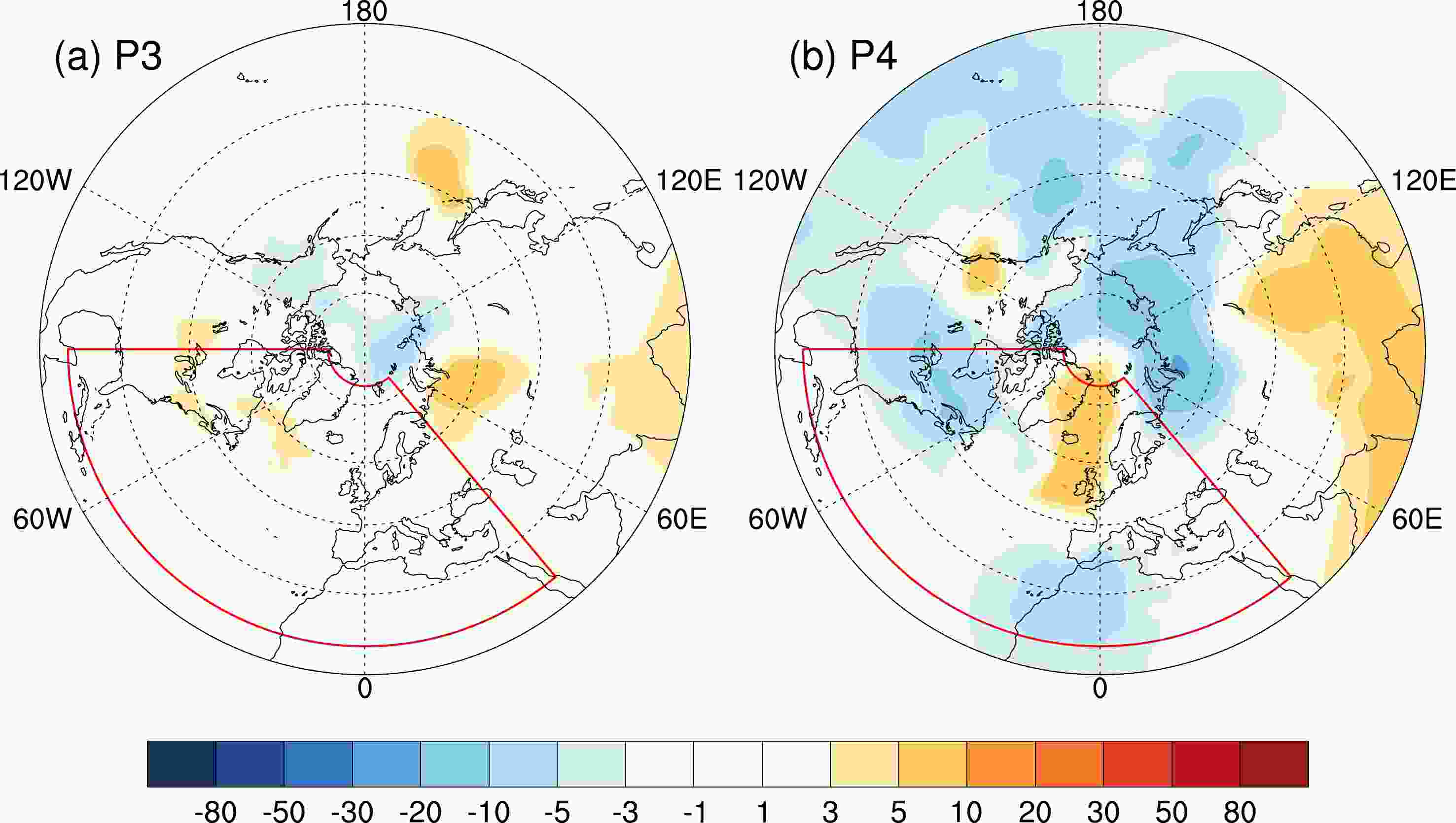

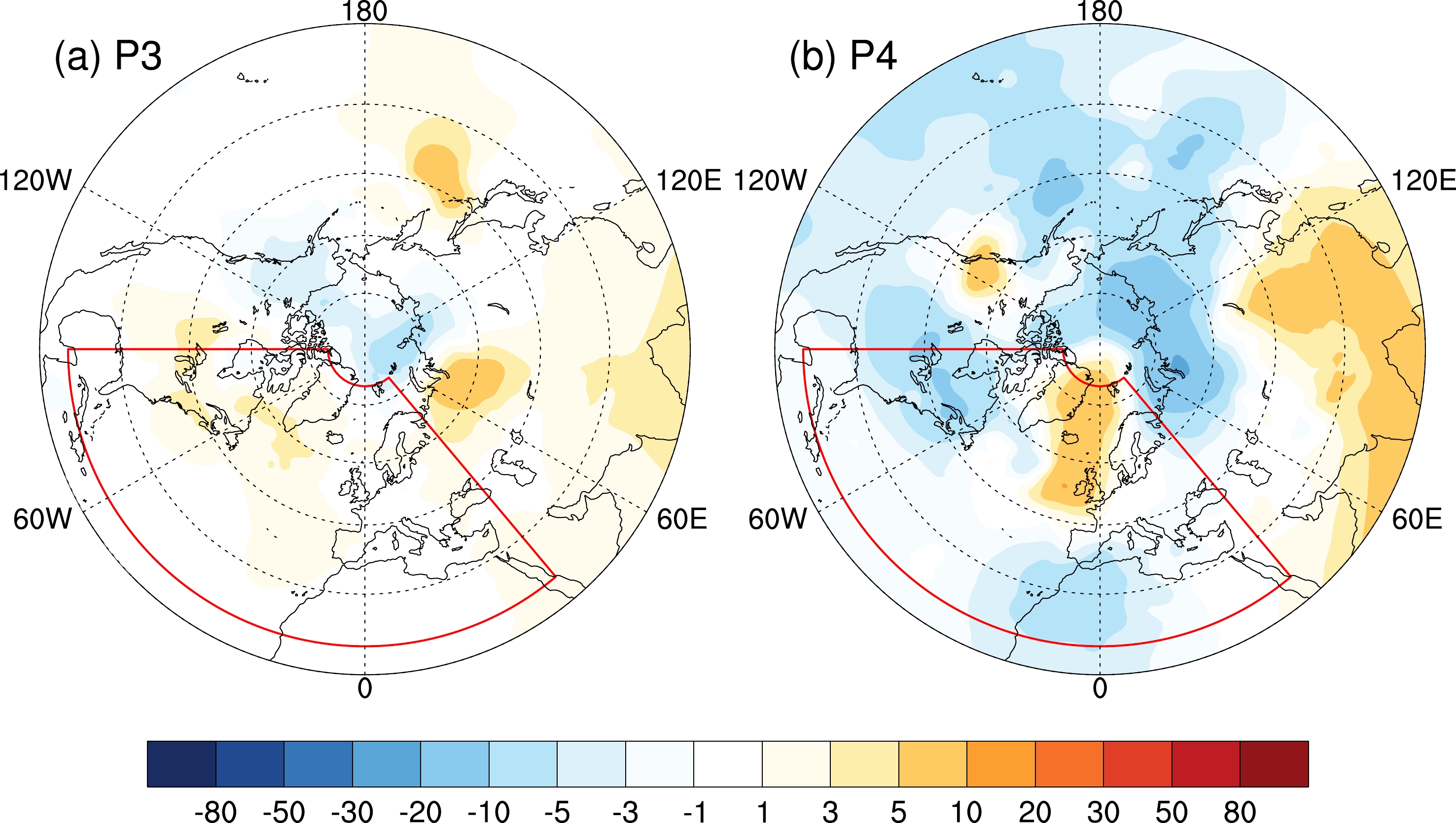
Figure 9.  The response of the 500-hPa potential vorticity advection (in terms of geopotential height, units: gpm d^–1) in (a) pentad 3 and (b) pentad 4. The red box in each panel indicates the North Atlantic sector (20°–80°N, 90°W–40°E).

Therefore, the influence of type-1 optimal SIC perturbations on this NAO+ event prediction can be concluded as follows. Both the latent heat flux and sensible heat flux experienced local adjustments due to Arctic SIC perturbations on the first day. During the 1st pentad, the temperature in the low troposphere has a local response due to diabatic processes. After that, the dynamic processes (horizontal temperature advection and vertical temperature convection) play crucial roles in modifying the temperature response. The Z500 has a baroclinic response to the temperature with Z500 increasing in warming sectors while decreasing in cooling areas in pentads 1−2. In pentads 3−4, the response in Z500 is mainly influenced by dynamic potential vorticity advection and finally exhibits a positive response in the northern North Atlantic sector. Therefore, the SLP around Greenland increases and underestimates the NAO+ event as a consequence.

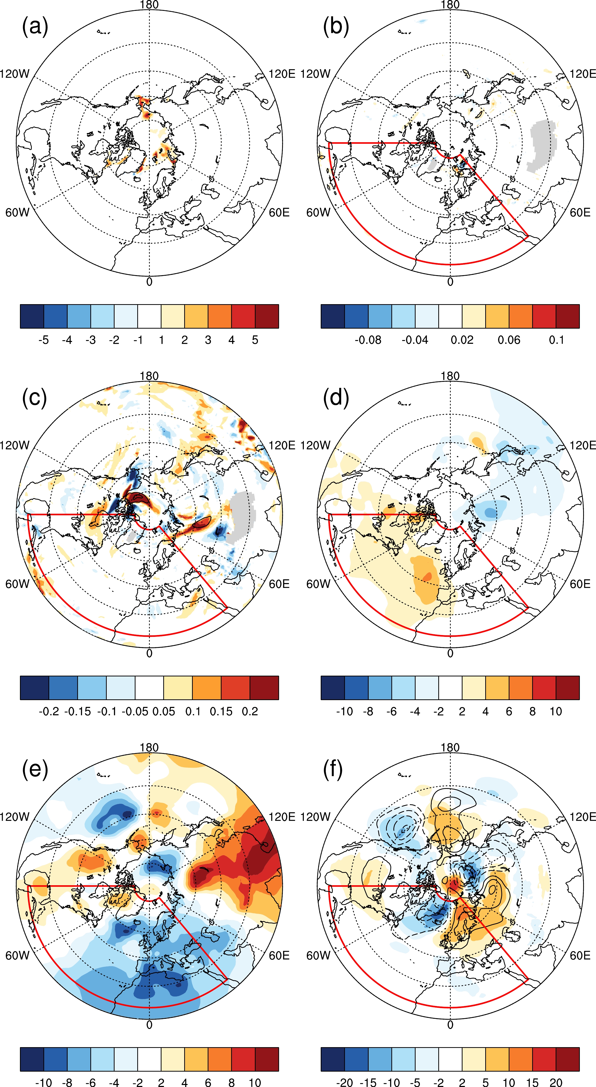
Regarding type-2 optimal SIC perturbations on NAO+ event prediction, their influence has been investigated similarly. As shown in Fig. 10a, on the first day, the turbulent heat flux increases in response to the Arctic SIC decline in the Greenland Sea, Barents Sea, and Bering Sea (Fig. 4b). The turbulent heat flux response warms the temperature in the low troposphere via diabatic processes in pentad 1. After that, the temperature response is mainly affected by horizontal temperature advection and vertical convective processes. During pentads 1−2, Z500 has a baroclinic response to the temperature by raising Z500 in warm sectors and declining Z500 in cooling areas. For pentads 3−4, the atmospheric dynamic process (potential vorticity advection) dominates the Z500 response. Finally, the 500-hPa geopotential height decreases in Greenland, as does the SLP in pentad 4. This strengthens the northern center of the NAO+ dipole and overpredicts the NAO+ event (Fig. 10f).

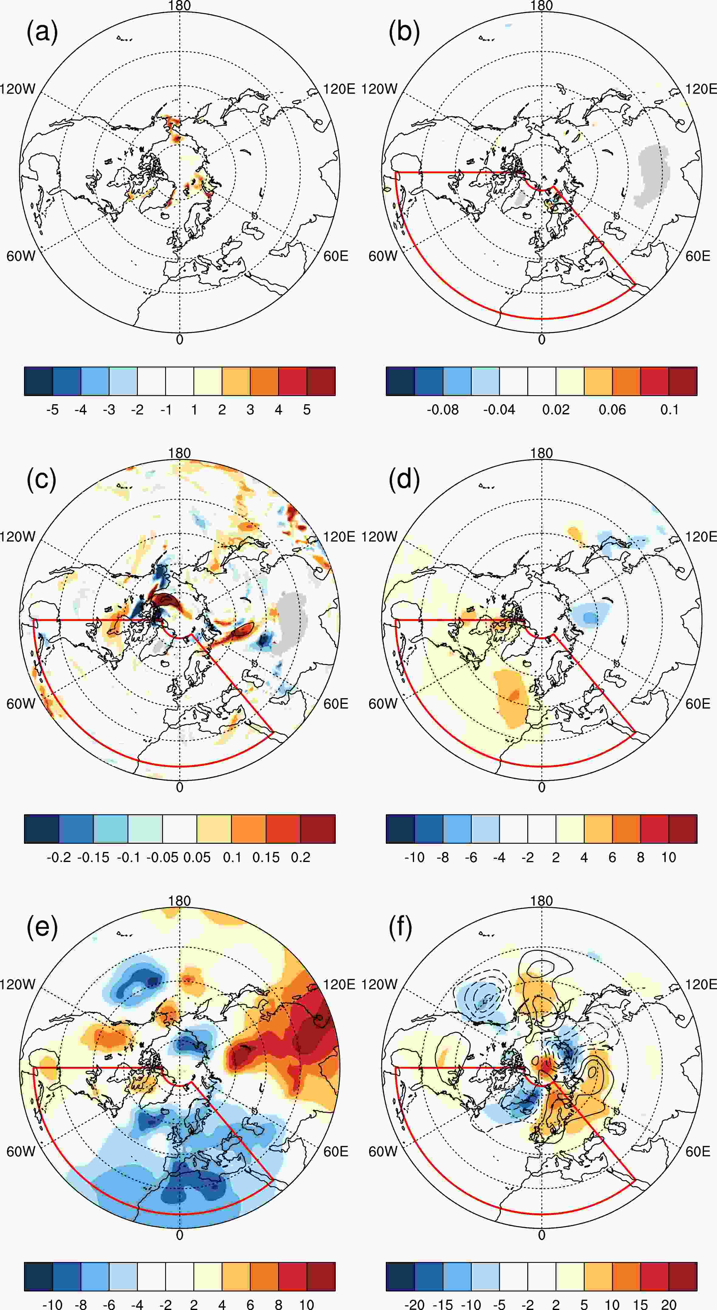
Figure 10.  Physical mechanisms associated with type-2 optimal Arctic SIC perturbations on the first simulated NAO+ event prediction. Panel (a) is the turbulent heat flux response on day 1 (units: W m^–2), while panels (b) and (c) illustrate the 700-hPa temperature response (shading, units: K) and Z500 response (CI = 0.2 gpm for (b) and CI = 4.0 gpm for (c)) during pentads 1 and 2, respectively. Panels (d) and (e) are the 500-hPa potential vorticity advection (in terms of geopotential height, units: gpm d^–1) during pentads 3 and 4, respectively. Panel (f) is the SLP response (shading, units: hPa) and Z500 response (CI = 40 gpm) in pentad 4. The red box in panels indicates the North Atlantic sector (20°–80°N, 90°W–40°E).

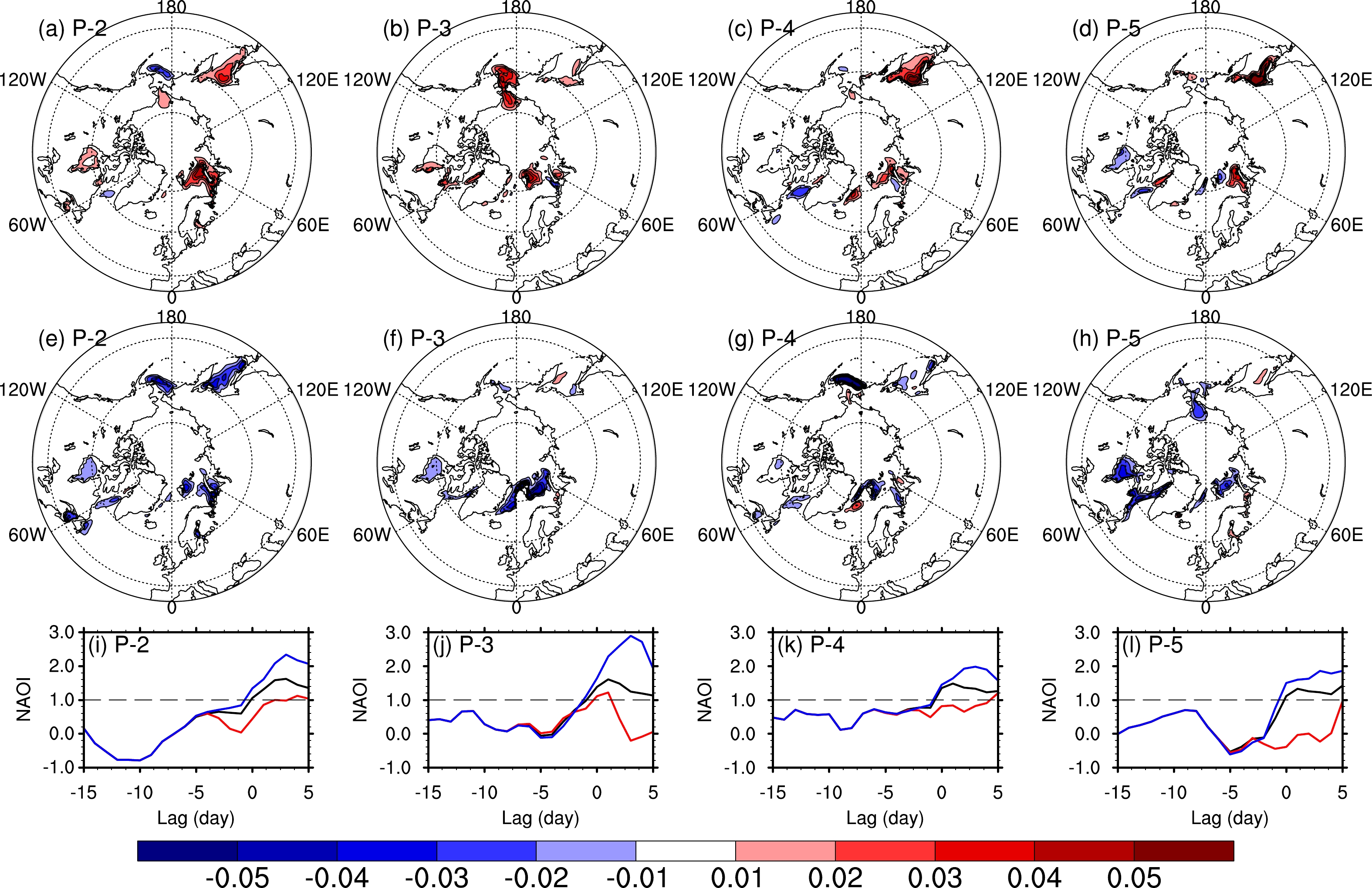
Similar processes have been applied to explore the influences of Arctic SIC on the remaining four NAO+ event predictions. There are two types of optimal Arctic SIC perturbations for each NAO+ event, mainly with positive SIC perturbations in the Barents Sea and Okhotsk Sea for type-1 and negative SIC perturbations in these regions for type-2 (Fig. 11). Similarly, type-1 optimal SIC perturbations would underestimate the NAO+ event and even make the event disappear, while type-2 optimal SIC perturbations overpredict the NAO+ events. However, it should be noted that there are some differences among the optimal SIC perturbations for these NAO+ event predictions. For example, there are obvious positive SIC perturbations in the Bering Sea in the type-1 optimal SIC perturbations for the 3rd NAO+ event, while there are obvious negative SIC perturbations in the Bering Sea in the type-2 optimal SIC perturbations for the 2nd and 4th NAO+ events. These differences are mainly due to the various initial atmospheric conditions while the optimal SIC perturbations have to match with the corresponding atmospheric states. Further diagnoses reveal that the mechanisms of optimal Arctic SIC perturbations on these NAO+ event predictions are similar to those in the first NAO+ event, which are not further stated here.

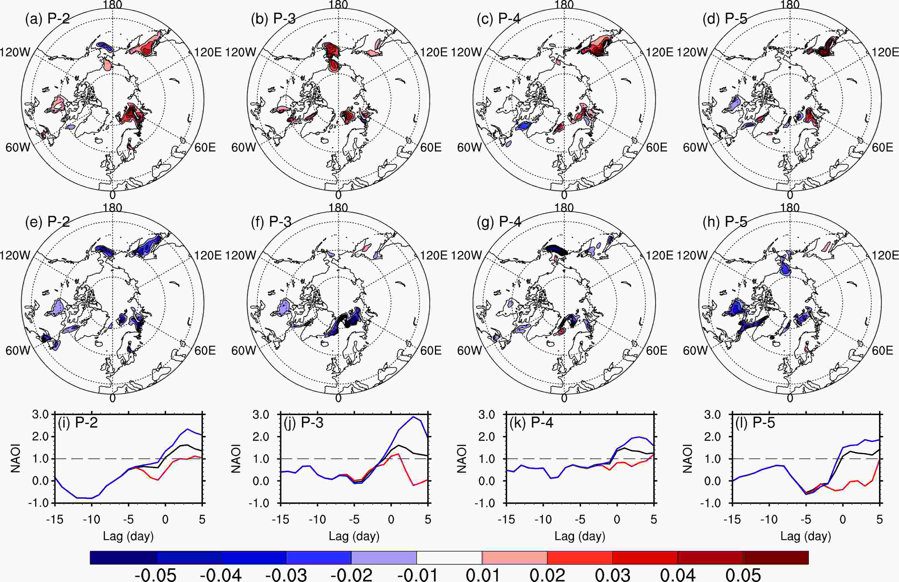
Figure 11.  Similar to those in Fig. 4, but for the (a) (e) (i) 2nd, (b) (f) (j) 3rd, (c) (g) (k) 4th, and (d) (h) (l) 5th simulated NAO+ event predictions.

In addition to the NAO+ events, the optimal Arctic SIC perturbations for NAO– event predictions are investigated. Similar to the investigations for NAO+ event predictions, the optimal SIC perturbations for the five NAO– event predictions are obtained by solving the corresponding nonlinear optimal problems.

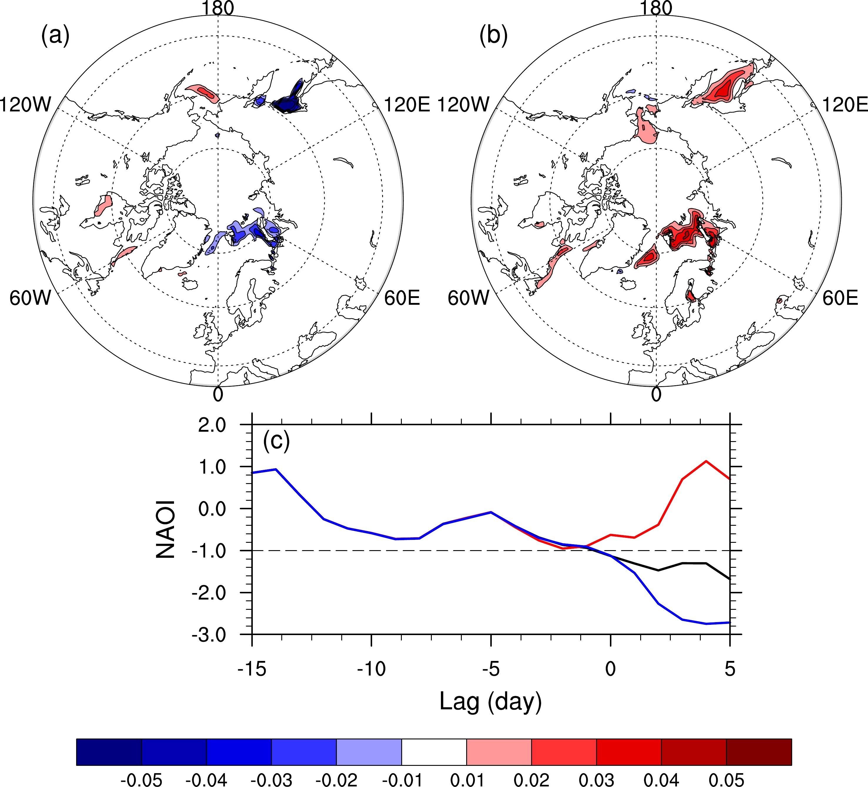
Taking the first NAO– event as an example, two types of optimal Arctic SIC perturbations are obtained and shown in Figs. 12a and b. They mainly show negative SIC anomalies in type-1 optimal SIC perturbations while positive SIC anomalies emerge in type-2 optimal SIC perturbations. Specifically, type-1 optimal SIC perturbations mainly show negative SIC perturbations in the BKS and west Okhotsk Sea, with some positive SIC perturbations in the Bering Sea. However, it mainly shows positive SIC perturbations in the Greenland Sea, BKS, and the east Okhotsk Sea in type-2 optimal SIC perturbations. Regarding their influences on NAO– event predictions, there is little influence on NAOI during the first three pentads (Fig. 12c). However, for the 4th pentad, the type-1 optimal SIC perturbation results in a higher NAOI than that in the reference state, which underestimates the NAO– event. However, type-2 optimal SIC perturbations result in a lower NAOI than that in the reference state leading to an overprediction of the NAO– event. This is also obvious in the SLP and Z500 response (Fig. S6).

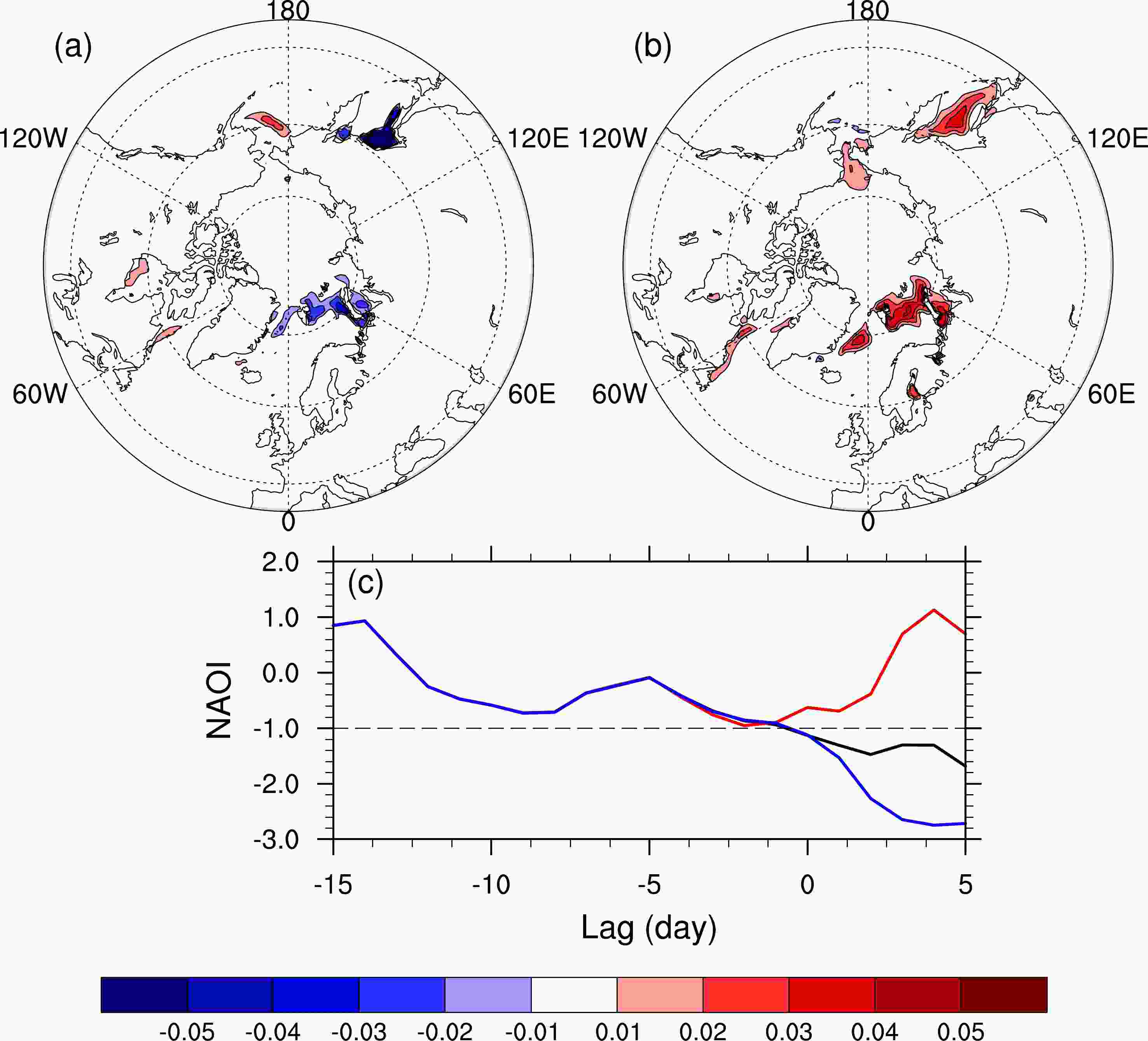
Figure 12.  (a) Type-1 and (b) type-2 optimal SIC perturbations for the first simulated NAO– event predictions. Panel (c) is the NAOI evolution derived in the reference state (black), type-1 optimal SIC perturbations (red), and type-2 optimal SIC perturbations (blue).

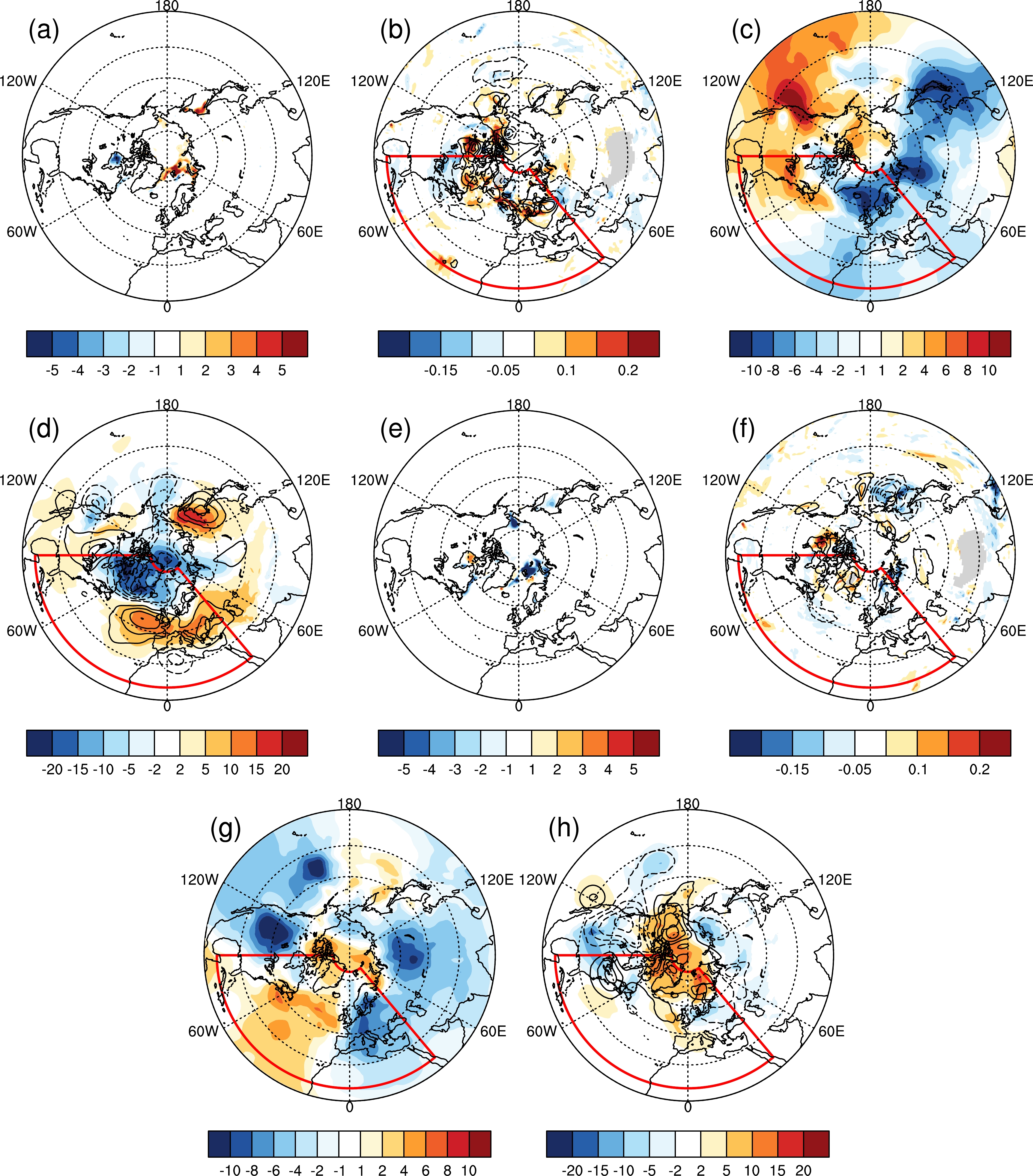
To illustrate the mechanisms of these Arctic SIC perturbations on this NAO– event prediction, similar processes have been investigated. As shown in Fig. 13a, there is increasing turbulent heat flux from ocean to air due to the negative SIC perturbations in the Greenland Sea, BKS, and Okhotsk Sea. The turbulent heat flux further warms the air in the lower troposphere due to the diabatic process during pentad 1. After that, the temperature in the lower troposphere is modified by horizontal advection and vertical convective processes, thus further influencing the 500-hPa geopotential height in pentad 2. During pentads 3−4, the Z500 response is mainly affected by the potential vorticity advection. Finally, type-1 optimal SIC perturbations trigger a negative-over-positive 500-hPa geopotential height dipole as well as the SLP in the North Atlantic sector, which underestimates the NAO– event in pentad 4 (Fig. 13d). Similarly, type-2 optimal Arctic SIC perturbations overpredict the NAO– event in pentad 4 but with smaller amplitudes compared with type-1 (Figs. 13e–h).

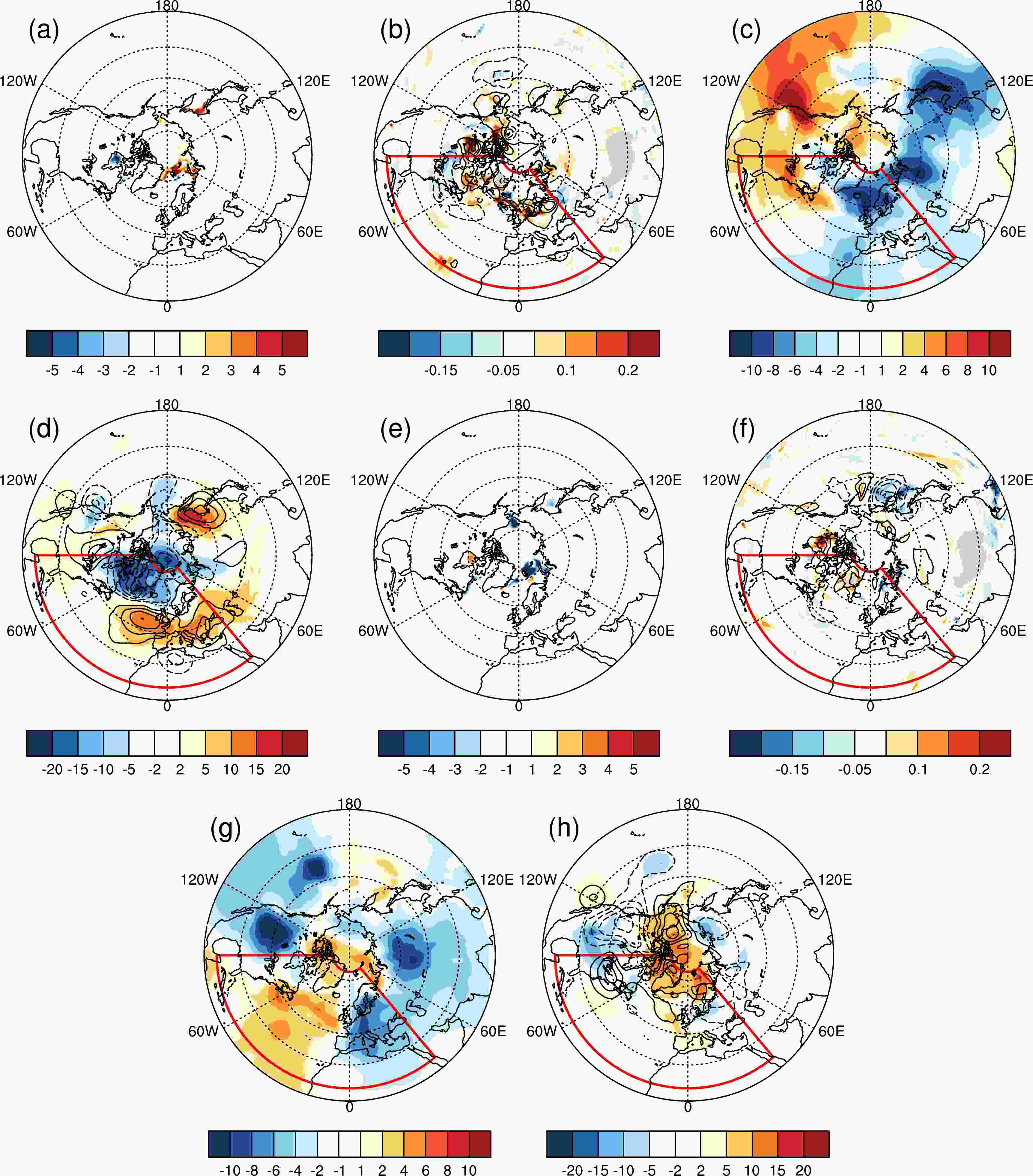
Figure 13.  Physical mechanism for optimal Arctic SIC perturbations on NAO– event predictions. Panel (a) is the turbulent heat flux response on day 1 (units: W m^–2) and (b) is the 700-hPa temperature response (shading, units: K) and 500-hPa geopotential height response (CI = 1.0 gpm) in pentad 2. Panel (c) is the potential vorticity advection (in terms of geopotential height, units: gpm d⁻¹) at 500 hPa during pentad 4. Panel (d) is the SLP response (shading, units: hPa) and Z500 response (CI = 40 gpm) in pentad 4. Panels (e)–(h) are similar to (a)–(d) but for type-2 optimal SIC perturbations. The red box in each panel indicates the North Atlantic sector (20°–80°N, 90°W–40°E).

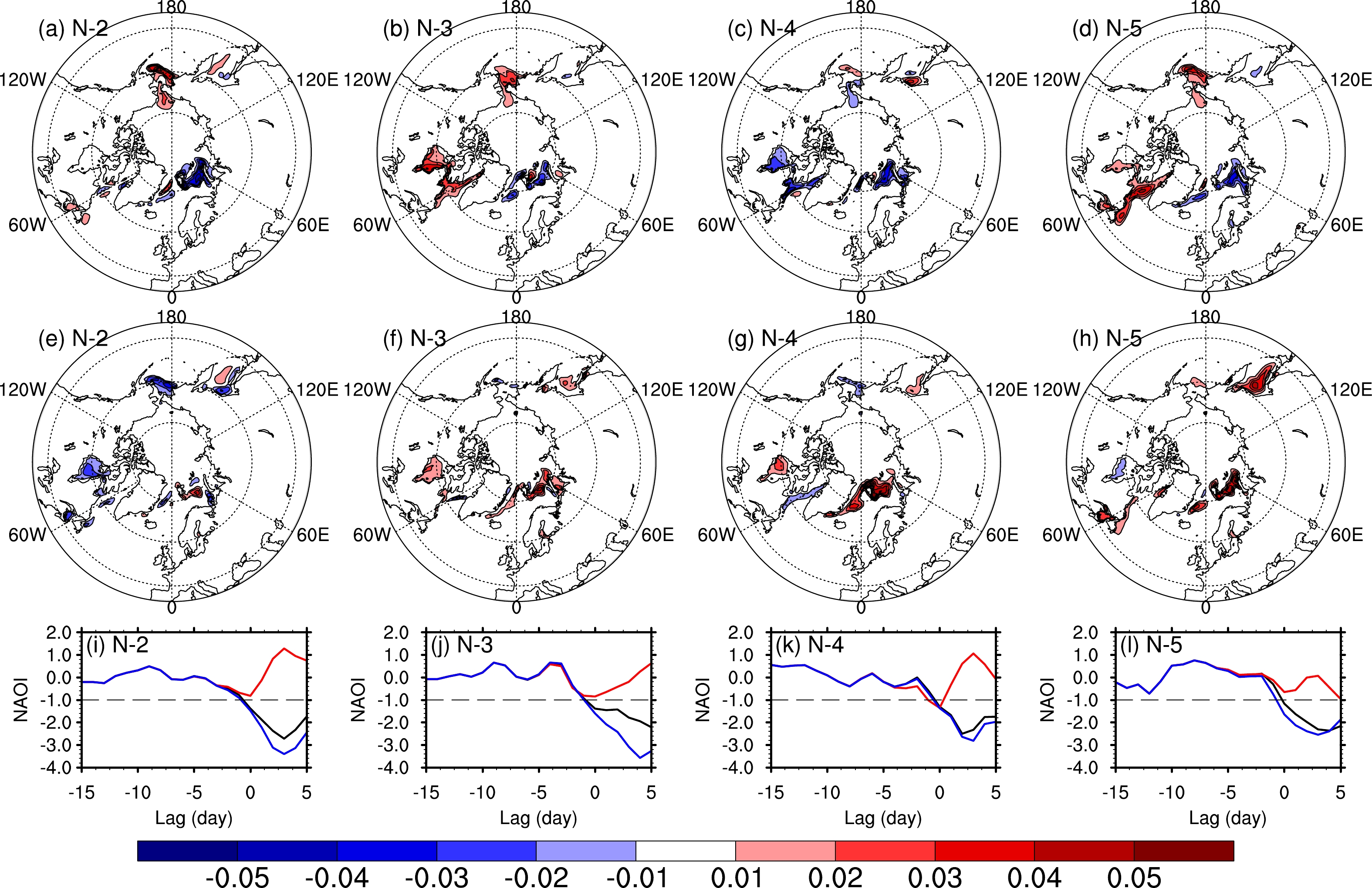
Moreover, the optimal Arctic SIC perturbations for the remaining four NAO– event predictions have also been investigated similarly. The two types of optimal Arctic SIC perturbations and their influences on NAO– event predictions are shown in Fig. 14. It is obvious that type-1 optimal SIC perturbations for these NAO– event predictions mainly show negative SIC anomalies in the Greenland Sea and Barents Sea, and they would like to underestimate the NAO– events and even disappear. However, the type-2 optimal SIC perturbations mainly show positive SIC anomalies in the Barents and Okhotsk Seas, and they would likely lead to a lower NAOI in pentad 4 and overpredict the NAO– events. However, there are still some differences among these optimal SIC perturbations. For example, there are some positive SIC anomalies in the Bering Sea for type-1 optimal SIC perturbations in the 2nd, 3rd, and 5th NAO– events, while type-2 optimal SIC perturbations for the 2nd NAO– event show some negative SIC anomalies in the Okhotsk and Bering Seas. These differences may be due to the different atmospheric initial conditions among these NAO– events. Further diagnoses show that the mechanisms of the optimal SIC perturbations on the corresponding NAO– event predictions are similar to those in the first NAO– event. This mechanism could be interpreted as the turbulent heat flux, acting in response to the SIC perturbations, serving to modify the low tropospheric temperature via diabatic processes in the first pentad. Horizontal and vertical temperature advection dominate the temperature response in pentads 2−3, allowing Z500 to have a consequent baroclinic response to the temperature perturbations. Subsequently, the dynamic potential vorticity advection becomes dominant in pentads 3−4. Finally, the Z500 demonstrates a positive (negative) geopotential height response in the northern North Atlantic sector, as does the SLP, which underestimates (overpredicts) the NAO– event.

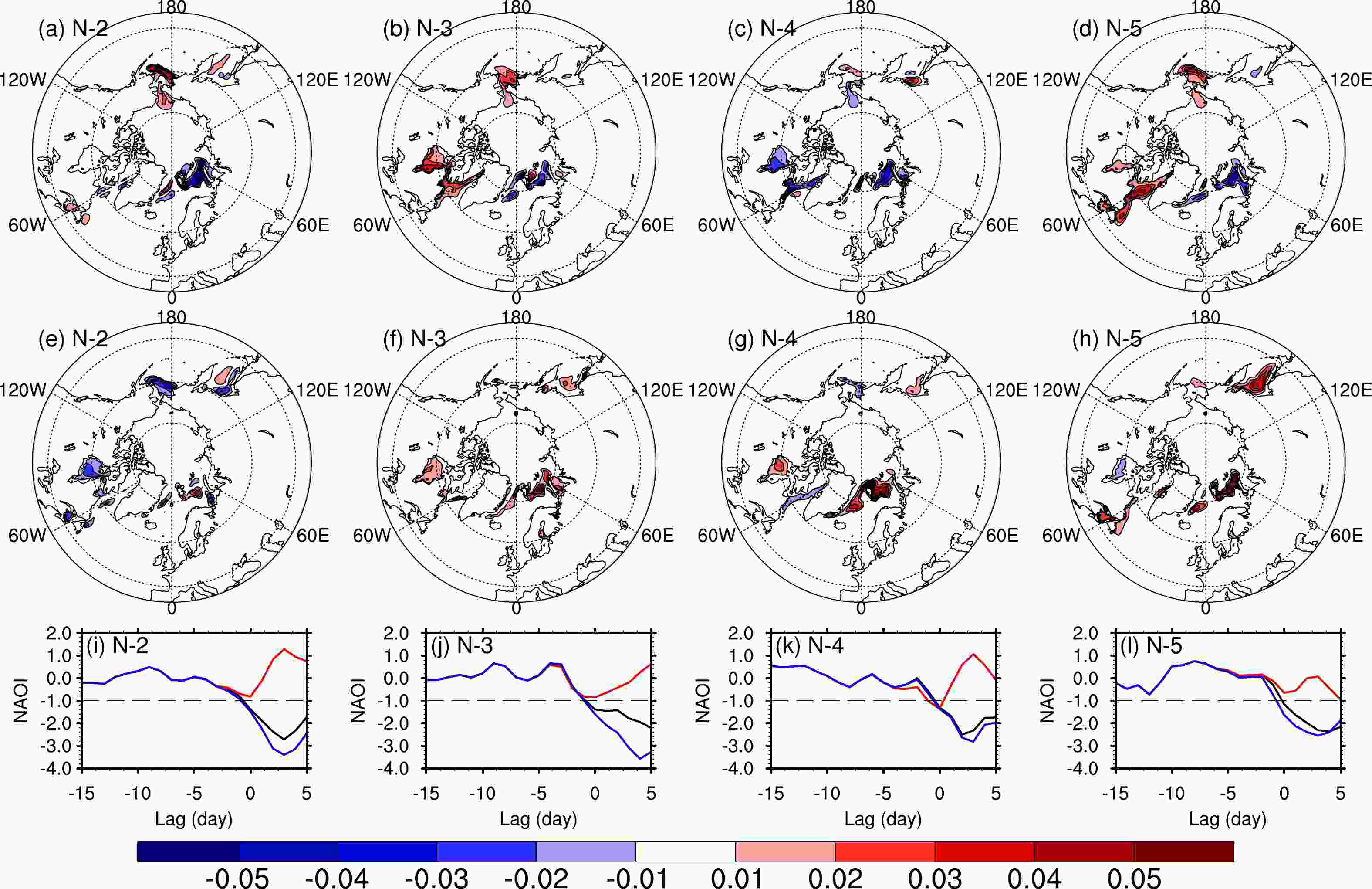
Figure 14.  Similar to those in Fig. 12, but for (a) (e) (i) 2nd, (b) (f) (j) 3rd, (c) (g) (k) 4th, and (d) (h) (l) 5th simulated NAO– event predictions.

In this investigation, we focused on the influence of Arctic SIC perturbations on NAO event predictions on subseasonal timescales. Utilizing the CAM4 model with climatological SST and SIC, we found that the model well describes NAO event evolution on subseasonal timescales in the control simulations. Five NAO+ and five NAO– events were selected from the control simulations and were further investigated to explore the influence of Arctic SIC on their predictions.

First, the response time for NAO events to Arctic SIC perturbations was determined with a series of sensitivity numerical experiments. Numerical results show that NAO demonstrates notable responses to Arctic SIC perturbations in 10 days and SIC perturbations have large influences on NAO formations when the SIC perturbations are 15 days ahead of the onset, indicating that Arctic SIC is a predictability source for NAO events on subseasonal timescales. After that, the CNOP-B approach was utilized to find the optimal Arctic SIC perturbations, which have the greatest impacts on NAO event prediction. The optimal SIC perturbations were obtained by solving the corresponding nonlinear optimal problem for each NAO event. Numerical results show that there are two types of optimal Arctic SIC perturbations for each NAO event, with type-1 optimal SIC perturbations tending to underestimate the NAO event and type-2 optimal SIC perturbations tending to overpredict the event in 4 pentads. The optimal SIC perturbations have greater influences on NAO event predictions compared with the random SIC perturbations under the same physical constraint. For NAO+ events, type-1 optimal SIC perturbations mainly show positive SIC anomalies in the Greenland Sea, Barents Sea, and Okhotsk Sea, while type-2 mainly exhibit negative SIC anomalies in these regions. However, for NAO– events, type-1 optimal SIC perturbations mainly show negative SIC anomalies in Greenland and the Barents Seas, while type-2 optimal SIC perturbations exhibit positive SIC anomalies in the Greenland Sea, BKS, and Okhotsk Sea. The type-1 optimal SIC perturbations almost share an opposite pattern to the type-2 optimal SIC perturbations for both NAO+ and NAO– events, although there are some slight differences among these optimal SIC perturbations due to the different atmospheric initial conditions. These optimal SIC perturbations also correspond to the ice-edge regions with strong SIC variations and large uncertainties in boreal winter, highlighting that sea-ice anomalies in both the Atlantic (Luo et al., 2016) and Pacific (Mesquita et al., 2011) sectors are important for the NAO.

Further diagnosis reveals that the optimal Arctic SIC perturbations modify the turbulent heat flux on the first day and affect the temperature in the low troposphere via diabatic processes. After that, the temperature in the lower troposphere is mainly modified by the dynamic temperature advection in pentad 2. During pentads 3-4, dynamic processes such as potential vorticity advection play a crucial role in modifying the Z500 response and finally form positive or negative 500-hPa geopotential height anomalies in pentad 4. The SLP demonstrates an equivalent barotropic response to that at 500 hPa and further influence the NAO intensity in pentad 4. These results are dependent upon the reference state of NAO events. As for the reference states without any NAO events, the solution to the optimization problem refers to the optimal precursor if it can trigger an NAO event onset. This will be explored in our future work.

Similar to previous studies, our results highlight the role of Arctic SIC on NAO event predictions. From a climatological perspective, many previous studies have revealed that Arctic SIC can affect NAO activities by modifying the temperature meridional gradients of temperature and potential vorticity as well as planetary wave activities in the North Atlantic sectors (Overland et al., 2011; Jaiser et al., 2012; Luo et al., 2019). Their results also indicate that Arctic SIC loss would result in a negative or negligible NAO response compared with atmospheric internal variability (Blackport and Screen, 2021; Siew et al., 2021; Warner et al., 2020). However, our results suggest that on subseasonal timescales, the NAO has positive responses to negative SIC anomalies in the Greenland Sea, Barents Sea, and Okhotsk Sea, and vice versa, while local dynamic and thermodynamic processes are crucial for NAO event prediction. The influence of thermal forcing on extratropical atmospheric circulations is complicated and includes multiple eddy feedback processes and flow dependencies. This indicates that both Arctic SIC and atmospheric internal variability are important for subseasonal NAO event prediction. We also highlight the matching mechanism between SIC perturbations and the atmospheric initial state for NAO event evolution. Moreover, our result indicates that the Greenland Sea, Barents Sea, and Okhotsk Sea may be sensitive areas for subseasonal NAO event predictions, which require further elaborate investigations in the future (Dai et al., 2019; Zhang et al., 2019, 2020).

It should be further noted that atmospheric initial perturbations are also crucial for subseasonal NAO predictions since subseasonal ensemble forecast systems usually utilize specific atmospheric initial perturbations generated by various approaches to improve forecast skills (Vitart et al., 2017). However, the influence of atmospheric initial perturbations on subseasonal NAO predictions is not discussed here. Nevertheless, our result indicates that the specific Arctic SIC perturbations may further improve the subseasonal NAO prediction skill. Additionally, as pointed out by many investigations, the stratosphere is a key process in linking the Arctic and mid-latitudes (Sun et al., 2015, 2022; Zhang et al., 2018). Their results indicate that the elaborate stratospheric process in numerical models plays a crucial role in describing the seasonal or longer linkage between the Arctic and mid-latitudes. But for timescales of 4 pentads, the low-top and coarse stratosphere in CAM4 may only have a negligible influence on the Arctic and mid-latitude linkage. We may further confirm our results with high-top models in the future. However, the feedback from atmospheric circulations to SIC variabilities cannot be estimated, since CAM4 is an atmospheric-only circulation model and the Arctic SIC is treated as a boundary condition. As revealed by Strommen et al. (2022), air–ice coupling might be important for simulating sea ice–NAO teleconnections. Therefore, the relationship between the NAO and sea ice should be further investigated with a fully coupled numerical model. Investigations of this nature may help to deepen the understanding of the mechanism of NAO event formation and provide scientific support for subseasonal NAO event predictions.

The authors are grateful to the editor and two anonymous reviewers for their helpful comments in improving this work. This study was supported by the National Natural Science Foundation of China (Grant Nos. 42288101, 41790475, 42005046, and 41775001). The calculations within this work were performed on TianHe-2 and the Atmospheric-Oceanic Numerical Simulation Platform. The authors appreciate the support of the National Supercomputer Center in Guangzhou (NSCC-GZ) and the High Performance Computing Center in the Department of Atmospheric and Oceanic Sciences, Fudan University.

Electronic supplementary material: Supplementary material is available in the online version of this article at https://doi.org/10.1007/s00376-023-2371-8.