


 DownLoad:


-
El Niño-Southern Oscillation (ENSO) is the dominant mode of interannual climate variability on Earth with a 2–7 yr irregular period (Philander, 1983; Tziperman et al., 1997; Neelin et al., 2000; McPhaden et al., 2006; Stein et al., 2010; Fang and Xie, 2020), reflected as an oscillation of cold and warm phases in the equatorial central to eastern Pacific. The evolution of ENSO exhibits a distinctive characteristic, as expressed during its onset in boreal spring, developing during summer and autumn, reaching its peak towards winter and decaying over the following spring (Tziperman et al., 1997; McGregor et al., 2012; Kim and An, 2021). The dependence of ENSO on the seasonal cycle is known as ENSO phase locking and can be measured through observations (Neelin et al., 2000; Stein et al., 2010; Chen and Jin, 2020; Fang and Zheng, 2021). Several studies found that more Coupled Model Intercomparison Project (CMIP) phase 6 reproduces ENSO phase locking performance over phase 5, yet simulations still differ markedly compared to observations, either peaking at the wrong calendar month or with weaker mature strength (Chen and Jin, 2021; Liu et al., 2021). Therefore, understanding the mechanisms responsible to ENSO phase locking is helpful to improve the simulation and prediction ability of a model.
Substantial efforts concerning this issue have been put forth over the past few decades. More recently, many studies explained that the seasonal modulation of ENSO instability is the key to the phase-locking phenomenon (Tziperman et al., 1997; Stein et al., 2010, 2014; Chen and Jin, 2020, 2021, 2022; Kim and An, 2021). Chen and Jin (2020) examined the mechanism for ENSO phase locking by adopting a conceptual recharge oscillator (RO) model and indicated that the seasonal variance of ENSO arises as a result of seasonal modulation of the sea surface temperature (SST) growth rate in the Niño-3.4 region (5°S–5°N, 120°–170°W). Nevertheless, it is found that many state-of-the-art climate models portray an unrealistic depiction of the growth rate (Chen and Jin 2021). It is worth noting that the seasonally varying SST growth rate tends to be minimal in the early spring and at a maximum in the autumn, with the maximum growth rate leading ENSO peaks by approximately 2–3 months (Li, 1997; Stein et al., 2010, 2014; Chen and Jin, 2021, 2022; Kim and An, 2021), which may elucidate the occurrence for ENSO mature phases becoming locked in the boreal winter (Li, 1997; Liu et al., 2021). Later, Kim and An (2021) proposed a seasonal energy index (SEI) based on a modified seasonally dependent RO model, indicating that ENSO events tend to peak with the largest SEI, which well illustrates the seasonal gap between the maximum SST growth rate and SST variance and renders an explicit explanation for ENSO phase locking.
Understanding the variation of SST is of great help in comprehending the evolution of SST growth rate. As the most salient seasonal movement in the tropical region, extensive studies have elucidated that the air-sea interaction induced by the meridional immigration of the intertropical convergence zone (ITCZ) acts as a great attribution to the SST annual cycle (Philander, 1983; Xie and Philander, 1994; Tziperman et al., 1997; Wang et al., 2004; Xie et al., 2018). It is also shown that the variation of the background state governed by the seasonal distribution of ITCZ in the equatorial Pacific plays a dominant role in the development of the SST growth rate (Levine and McPhaden, 2015). Seasonal changes in the combination of trade winds, ocean currents, surface heat flux, thermocline depth, and upwelling bring about the variation of SST and the seasonal modulation of the SST growth rate. Over the past few years, considerable efforts have been made to estimate the variation of SST and growth rate. Since the mixed layer ocean heat budget equation is used as a direct tool for diagnosing the SST variability as well as investigating different oceanic processes in ENSO dynamics (Wang and McPhaden, 1999, 2000, 2001; Huang et al., 2010, 2012; Chen et al., 2016a, b, 2017), Ren and Wang (2020) analyzed the SST growth rate by combining recharge oscillator theory (Jin, 1997; Jin et al., 2006) and the mixed layer heat balance equation in the equatorial Pacific, concluding that the thermocline feedback (TH) and thermodynamic damping (TD) are two major positive and negative contributors for growth rate variation, with the zonal advective feedback (ZA) and mean advective damping playing the secondary roles. Chen and Jin (2022) further investigated this topic using a similar method as Ren and Wang (2020) and identified that the seasonal cycle of the SST growth rate mainly relies on the ZA and TH. However, their estimate of the mixed layer depth (MLD) was fixed at a certain value as it was in Stein et al. (2010) and Boucharel et al. (2015). Our analysis indicates that there are spatial and temporal differences in the MLD in the Niño-3.4 region over the past 40 years, which cannot be ignored. Particular attention is directed toward the consequences and importance of considering the varying MLD in diagnosing the SST growth rate.
The remainder of this paper is arranged as follows: Section 2 introduces the data and methods employed in this research. Section 3 illustrates the annual cycles and seasonal variations of the dynamic and thermodynamic processes of the oceanic mixed layer heat budget equation and further demonstrates the characteristics of the SST growth rate and its contributing factors that are regulated by the seasonal migration of the ITCZ. Section 4 summarizes the paper with a discussion of the findings.
-
In this study, monthly variables during 1981–2020 are obtained from three observational and reanalysis datasets including: 1) oceanic currents, potential temperature, vertical velocity, MLD, and surface heat flux from the National Centers for Environmental Prediction (NCEP) Global Ocean Data Assimilation System (GODAS) on a 1/3°
$ \times $ 1° grid within 10° of the equator and with 40 vertical levels (Behringer et al., 1998); 2) shortwave radiation from the NCEP/DOE (Department of Energy) Reanalysis 2 on a 2.5°$ \times $ 2.5° grid (Kanamitsu et al., 2002); 3) precipitation from the Climate Prediction Center (CPC) Merged Analysis of Precipitation (CMAP) on a 2.5°$ \times $ 2.5° grid (Xie and Arkin, 1997). Thermocline depth is not provided in those products, and thus calculations are performed using the GODAS dataset based on the 20°C isotherm criterion. Seasonal movement of ITCZ is characterized by the shift of 15°S–15°N precipitation centroid (Voigt et al., 2016) estimated from the CMAP monthly averaged precipitation dataset in from 120° to 170°W. Anomalies are analyzed by removing the 1981–2020 climatology. -
To examine the dynamical and thermodynamical processes affecting the SST variability, the oceanic mixed layer heat budgets are investigated in this study. The temperature tendency equation is expressed as follows (see details in Appendix):
where
${T_a}$ and$ { {{\partial {T_a}}}/{\partial t} } $ are the mixed layer temperature and its tendency ($ {T_t} $ ) and subscript$ a $ represents the vertical average between the sea surface and the bottom of the mixed layer. The forcing term$F$ mainly consists of zonal advection [${Q_u} = - {u_a} ({{\partial {T_a}}}/{{\partial x}})$ ], meridional advection [${Q_v} = - {v_a} ({{\partial {T_a}}}/ {{\partial y}})$ ], vertical entrainment (${Q_w}$ ), vertical diffusion (${Q_{zz}}$ ), and surface heat flux caused by radiation (${Q_q}$ ). Climatology is further removed from each term of Eqs. (1) and (2), and is written as:Note that,
$ Q'_u $ consists of three components, namely zonal advective feedback [climatological temperature by anomalous zonal currents,$ - u'_a({{\partial \overline {{T_a}} }}/{{\partial x}}) $ ],${\overline U}T' $ [climatological zonal currents by anomalous temperature,$ - \overline {{u_a}} ({{\partial T'_a}}/{{\partial x}}) $ ], and nonlinear processes. Nevertheless, closure of the heat balance equation may not be completely guaranteed due to the uncertainty of data assimilation or errors arising from the parameterization scheme of simulated vertical processes (Kim et al., 2007; Huang et al., 2010). -
The recharge theory proposed by (Jin, 1997) is adopted in this case to diagnose the SST growth rate in the Niño-3.4 region. The linear RO framework can be described as:
Here,
$ {h'} $ is the thermocline depth anomaly within 1° of the equator across the Pacific (120°E–80°W). In Eqs. (5) and (6), the coefficient R is the SST growth rate, the parameters$ \gamma $ ,$ \alpha b $ , and r represent the thermocline feedback, equatorial ocean adjustment, and damping process, respectively (Jin, 1997; Timmermann et al., 2018; Kim and An, 2021). Combining the RO model and mixed layer temperature tendency equation, the diagnostic Eq. (5) can be expressed as follows:Thus, there are two approaches for calculating the SST growth rate as mentioned in Eqs. (5) and (7). The latter provides an opportunity to further illustrate the different processes in
${F'}$ modulating the variation of SST growth rate. This will be demonstrated in section 3 in detail. -
Before starting, we note that the variable of MLD works throughout Eq. (2). To explore the variation of MLD in the Niño-3.4 region, this paper performs a 40-year analysis.
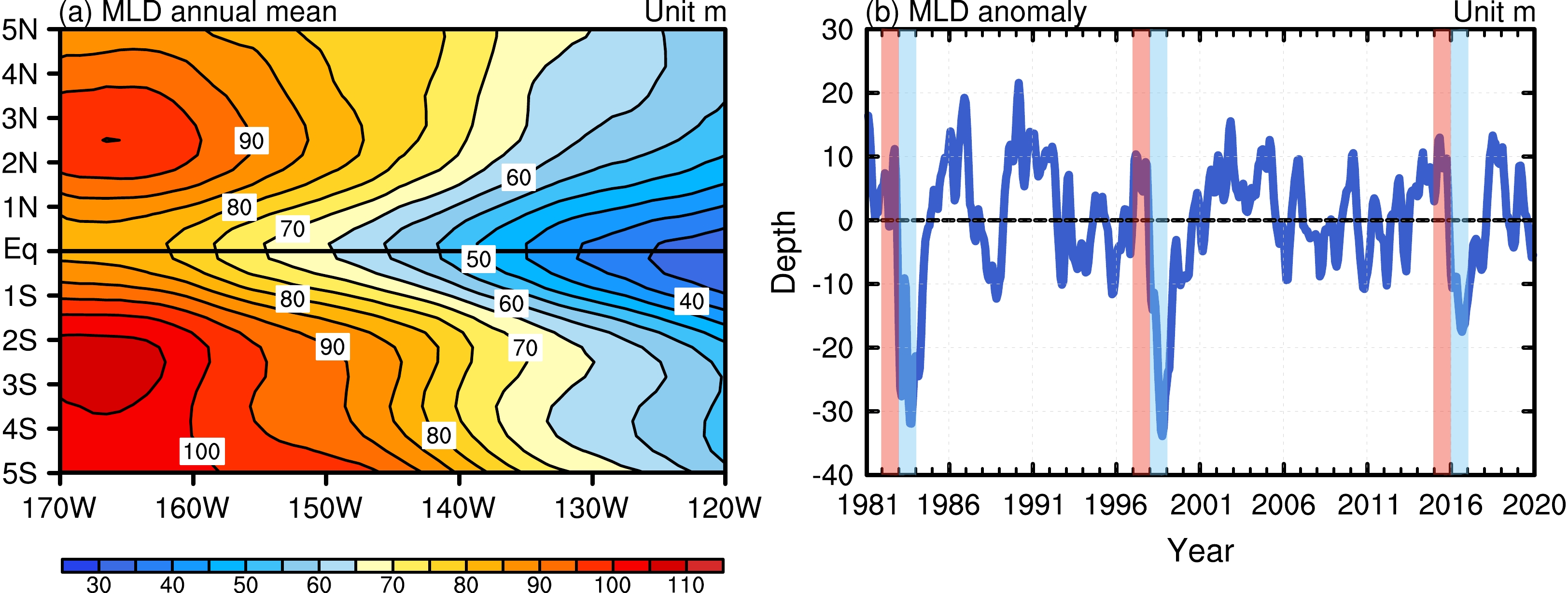
Results based on the data derived from GODAS reveal that the annual mean of MLD is found to vary from 30 to 110 m (Fig. 1a), accompanied by a decreasing gradient from west to east while being shallower on the equator than off the equator. In addition, the MLD fluctuates with time as well (Fig. 1b). Here, it is necessary to pay attention to the impact of MLD variations, as its spatial and temporal differences have been ignored. The MLD was defined at 50 m in the Niño-3.4 region according to previous studies (Ren and Wang, 2020; Chen and Jin, 2022). Next, we will take the SST as an example to compare the differences in adopting distinct MLD selection criteria.
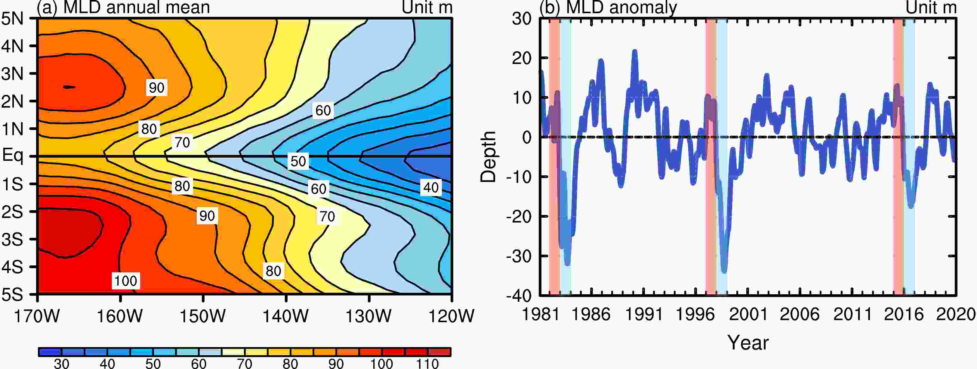
Figure 1. (a) The annual mean MLD in the Niño-3.4 region during 1981–2020 (units: m). The contour interval is 5 m for MLD. (b) The area-averaged anomalous MLD in the Niño-3.4 region during 1981–2020 (units: m). Three super ENSO events of 1982–83, 1997–98, and 2015–16 are shaded, where red ones represent the El Niño events and blue shades are La Niña events, respectively. A 3-month running mean has been applied in both plots.
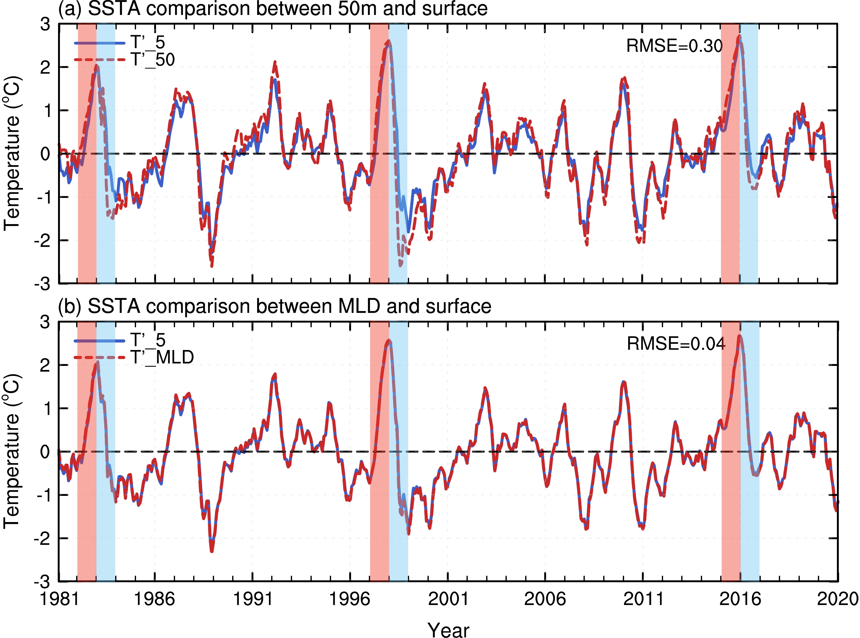
Figure 2 displays the time evolution of the area-averaged SST anomaly (SSTA), which was calculated with the variable MLD and fixed at 50 m in the Niño-3.4 region compared to the SSTA at 5 m during 1981–2020, respectively. It is obvious to see that
$ T'_{\_50} $ has a certain deviation from$T'_{\_5} $ , as this pattern can be found in three super ENSO events as well. Meanwhile, the root-mean-square error (RMSE) between$ T'_{\_{\text{MLD}}} $ and$ T'_{\_5} $ is much smaller than the one between$ T'_{\_50} $ and$ T'_{\_5} $ . Hence, considering the variation of MLD in the diagnostic process is more capable and accurate in characterizing the real situation of the surface. Note that, the analysis of the results of ocean heat balance is not sensitive to the selection criteria for the location of the bottom of the mixed layer (Huang et al., 2010). The selection criterion from GODAS is based on a buoyancy difference of 0.03 kg m–3 with the sea surface. It has been found that either temperature differences or density differences are alternatives used to reveal the variation of MLD (Kara et al., 2000; Thomson and Fine, 2003; Huang et al., 2010).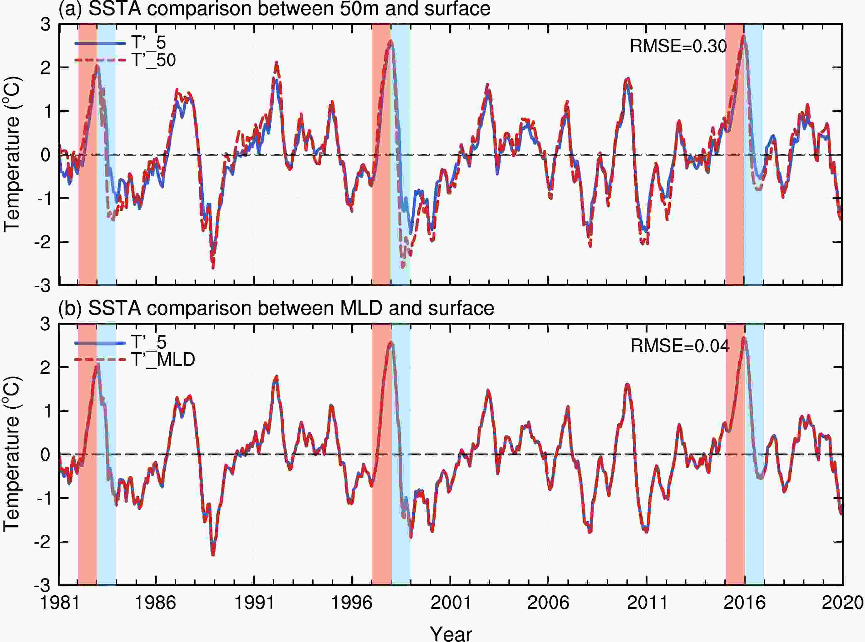
Figure 2. (a) Comparison between
$T'_{\_5}$ (averaged SSTA in the Niño-3.4 region at 5 m, blue solid line) and$T'_{\_50}$ (area averaged SSTA from sea surface to the fixed MLD at 50 m in the Niño-3.4 region, red dotted line). (b) Comparison between$T'_{\_5}$ and$T'_{{\text{\_MLD}}}$ (area averaged SSTA from sea surface to the varying MLD bottom in the Niño-3.4 region, red dotted line). Shaded bars represent three super ENSO events of 1982–83, 1997–98, and 2015–16, where red ones denote the El Niño events and blue shades are La Niña events, respectively. A 3-month running mean has been applied to both plots. -
The previous subsection discussed the spatial and temporal differences of MLD over the past 40 years and the advantages of considering its variability. After that, the annual mean of the mixed layer heat budgets in the Niño-3.4 region of each term in Eq. (2) is discussed.
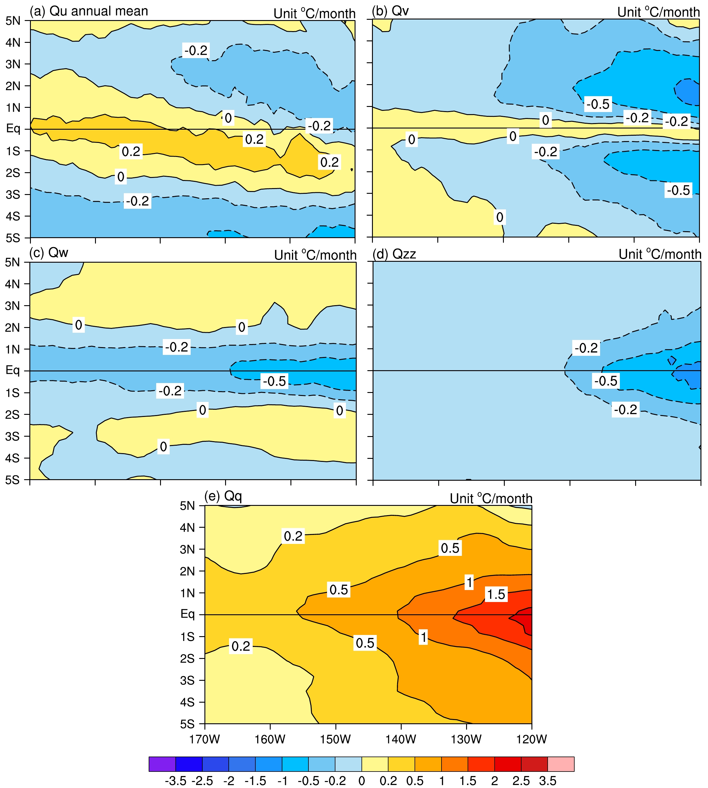
It is apparent that the strong heating by
${Q_q}$ (Fig. 3e) acts as the main positive contributor across the Niño-3.4 region with maximum amplitude over 2°C month–1 near 120°W. There is an increasing gradient of${Q_q}$ from west to east owing to the influence of surface radiation. That is because a cold tongue is established in the east and a warm pool in the west over the equatorial Pacific under the climatic background. Due to the effects of the Walker Circulation, the eastward sea surface receives more solar shortwave radiation than the west, accompanied by less outward longwave radiation due to the cooler sea surface in the east. The positive contributions of annual mean surface heat flux caused by radiation (${Q_q}$ ) and zonal advection (${Q_u}$ ) (Fig. 3a) along the equator are balanced by several cooling processes from meridional advection (${Q_v}$ ) (Fig. 3b), vertical diffusion ($ Q_{zz} $ ) (Fig. 3d), and vertical entrainment ($ Q_{w} $ ) (Fig. 3c) to a substantial extent. Typically,${Q_u}$ plays a negative role within 2° of equator while the maximum cooling centers of${Q_v}$ exist near 2°N with magnitudes of over 1°C month–1 and amplitudes of over 0.5°C month–1 near 2°S, close to the eastern Pacific. In contrast, cooling centers from${Q_w}$ and${Q_{zz}}$ are primarily concentrated near the equator (Figs. 3d, e). Although both of them are dynamic processes in the vertical direction,${Q_{zz}}$ has a greater cooling effect at a rate of 1°C month–1 approaching 120°W than${Q_w}$ . At the same time,${Q_{zz}}$ goes along with a broader meridional extension than${Q_w}$ as well. As for the vertical entrainment process (Fig. 3c), it is a narrow strip constrained within 3° of the equator, mainly resulting from the upwelling caused by Ekman transport.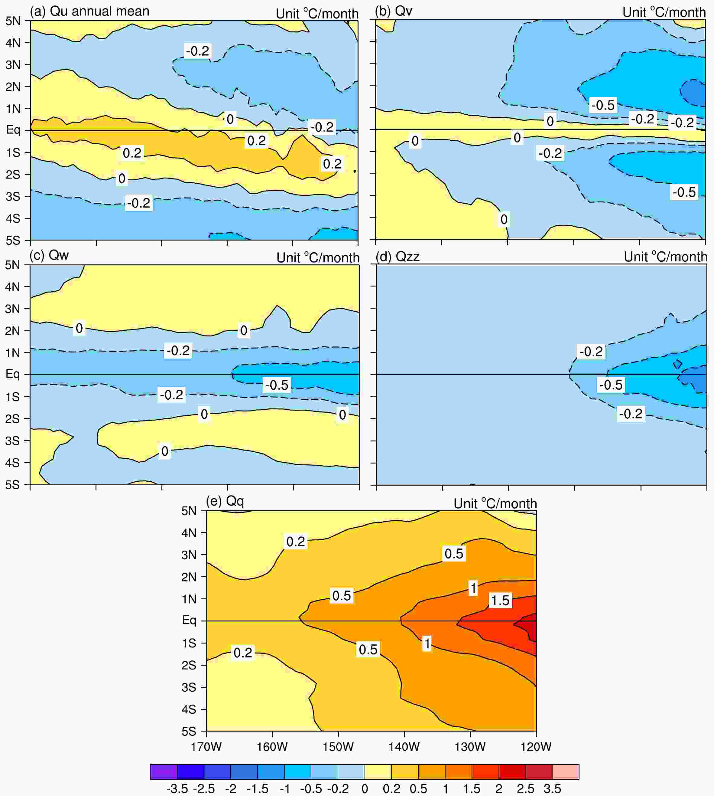
Figure 3. Annual mean of the mixed layer heat budgets for (a)
${Q_u}$ , (b)${Q_v}$ , (c)${Q_w}$ , (d)${Q_{zz}}$ , and (e)${Q_q}$ in the Niño-3.4 region during 1981–2020 (units: °C month–1). Positive areas are surrounded by solid lines and negative areas are circled by dotted lines. Irregular contour intervals are 0, ±0.2, ±0.5, ±1, ±1.5, ±2, ±2.5, and ±3.5°C month–1. A 3-month running mean has been applied to all plots. -
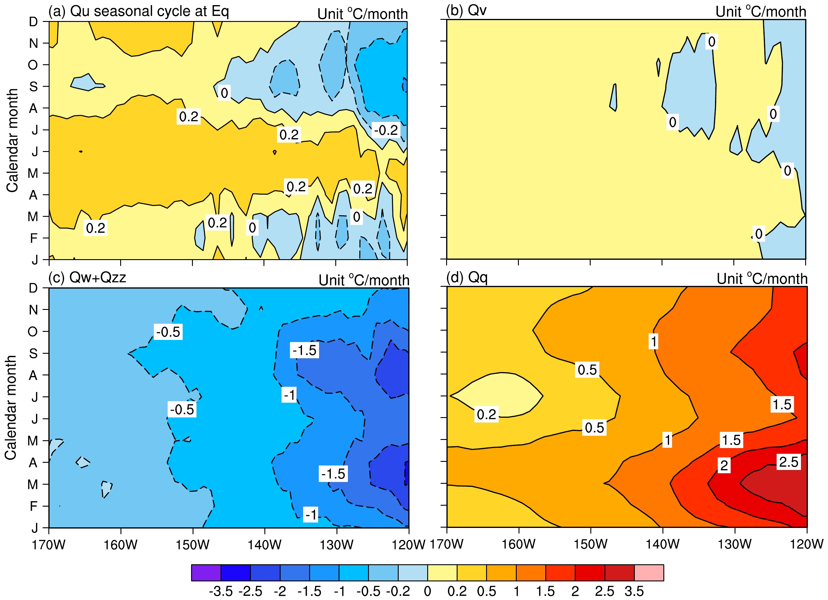
This subsection focuses on the seasonal cycle from the right-hand terms of the mixed layer heat budget equation at the equator (0°). As shown in Fig. 4, the forcing terms contributing to the variation of temperature tendency present noticeable seasonal cycles in the central to eastern Pacific.
${Q_u}$ produces a cooling effect from July to March and makes a positive contribution from April to June near east of 150°W with the maximum positive and negative amplitude appearing around May and September (Fig. 4a). The heating by zonal advection generally occupies the central Pacific all year round. According to the previous statistical analysis (Wang and McPhaden, 1999, 2000, 2001), the southward current in the central Pacific is salient throughout most of the year, while the northward flow near the eastern Pacific tends to peak from May to December. Thus, the seasonal variation of${Q_v}$ only weakly contributes to the temperature tendency (Fig. 4b). It is easy to capture a prominent semiannual cycle in${Q_q}$ due to the regulation from solar shortwave radiation with the maximum amplitude occurring in the boreal spring and the second-largest magnitude taking place in September close to 120°W (Fig. 4d). The heating effect from${Q_q}$ is quite intensely inclined eastward, which is the result of a shallower MLD and a relative decrease in cloudiness inherent to the eastern Pacific. Evidently,${Q_q}$ makes the most critical positive contribution to the mixed layer temperature tendency at a rate of 0°C–2.5°C month–1, noting that this is widely balanced by a cooling effect of terms of${Q_w}$ and${Q_{zz}}$ (Fig. 4c). Seasonal cycles for both of the vertical processes are negative throughout the year followed by two maximum magnitudes exceeding 2°C month–1 that appear during boreal spring and autumn. The cooling sources from${Q_w} + {Q_{zz}}$ are more pronounced further east in the equatorial Pacific all year round, where the MLD distribution is relatively shallow with a larger SST vertical gradient as well.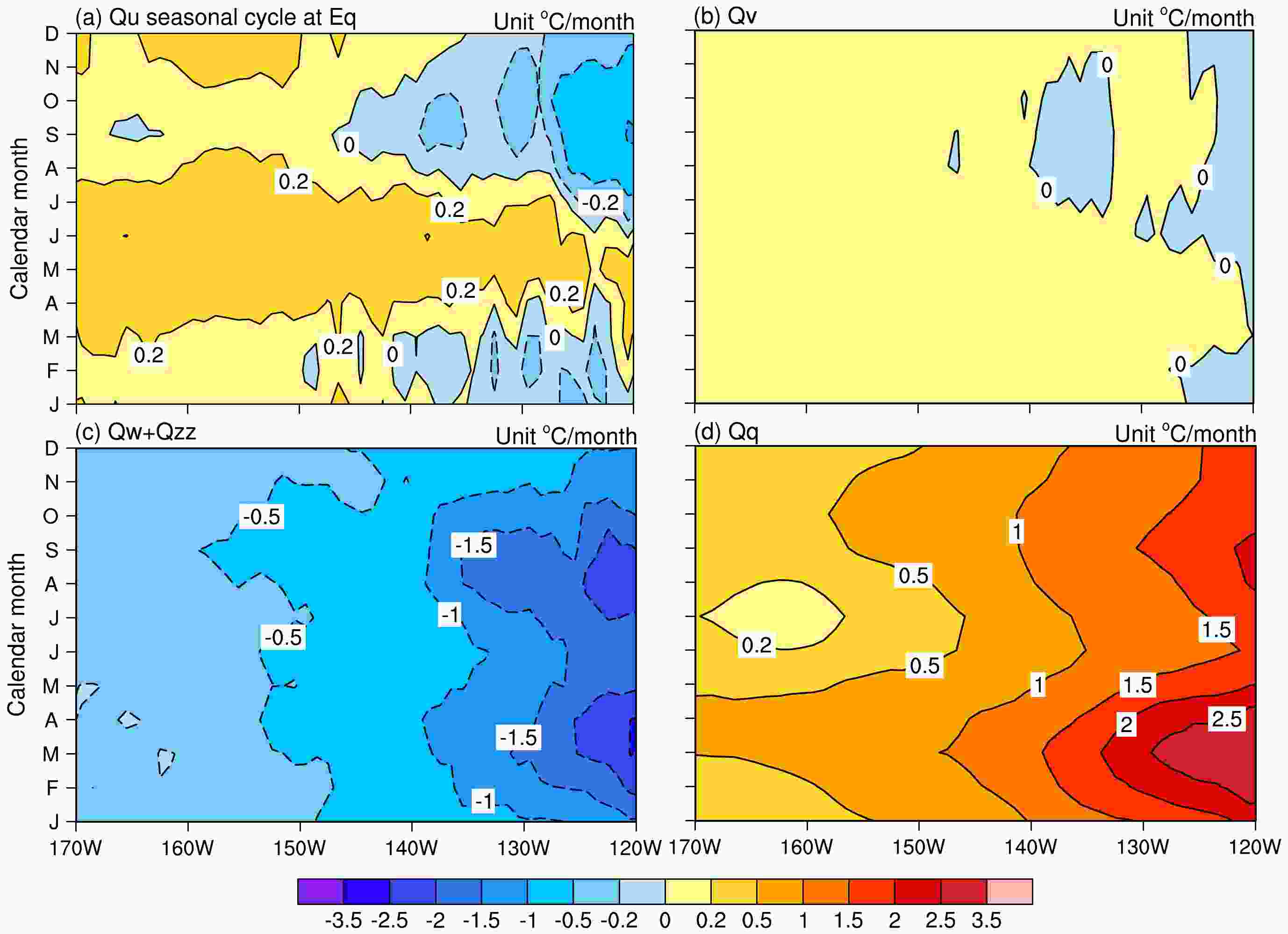
Figure 4. Seasonal cycles of the mixed layer heat budgets for (a)
${Q_u}$ , (b)${Q_v}$ , (c)${Q_w} + {Q_{zz}}$ , and (d)${Q_q}$ in the equatorial Pacific (0°) during 1981–2020 (units: °C month–1). Irregular contour intervals are 0, ±0.2, ±0.5, ±1, ±1.5, ±2, ±2.5, and ±3.5°C/month. A 3-month running mean has been applied to the plots. -
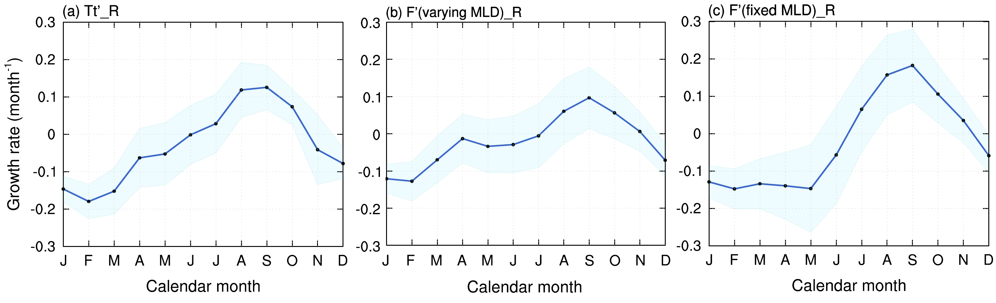
Based on the RO theory (Jin, 1997), two approaches to investigate the SST growth rate in the Niño-3.4 region were outlined in Eqs. (5) and (7). Growth rates estimated by linear regression utilizing the anomalous mixed layer temperature tendency and external forcing terms are performed by considering the variation in MLD. Generally speaking, both
$ T'_t\_R $ and$ {F'}({\text{varying MLD}})\_R $ exhibit similar characteristics (Figs. 5a, b), i.e., the positive growth rate peaks in September and the most negative one occurs in the early spring, which is reasonably consistent with previous studies (Li, 1997; Stein et al., 2010; Kim and An, 2021; Chen and Jin, 2022). However, there is a bias between growth rates calculated by forcing terms with fixed and varying MLD. The seasonal cycle of$ {F'}({\text{fixed MLD)}}\_R $ tends to be the strongest during the boreal autumn still, but the weakest growth rate shifts to May with indistinguishable differences in the four former months (Fig. 5c). This indicates that it is of great importance for considering the variation of MLD as a factor in diagnosing and analyzing the SST growth rate, a consideration that has been neglected by previous researchers (Boucharel et al., 2015; Ren and Wang, 2020; Chen and Jin, 2022).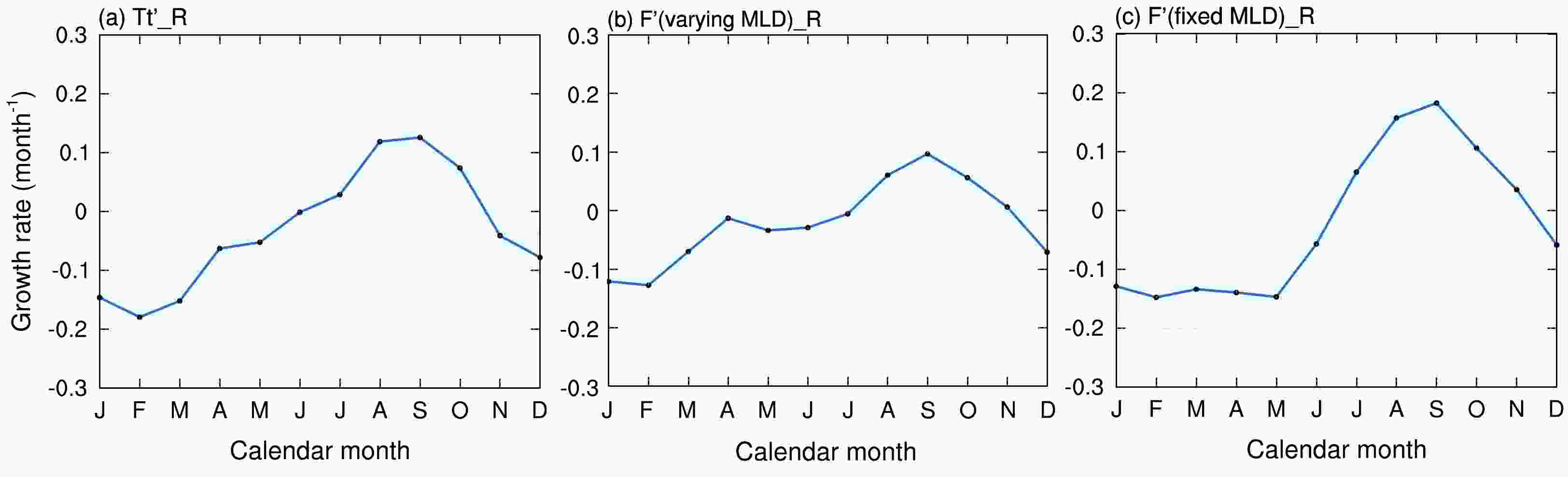
Figure 5. Curves with dots depict the seasonal cycle of the SST growth rate in the Niño-3.4 region diagnosed from (a) the anomalous mixed layer temperature tendency
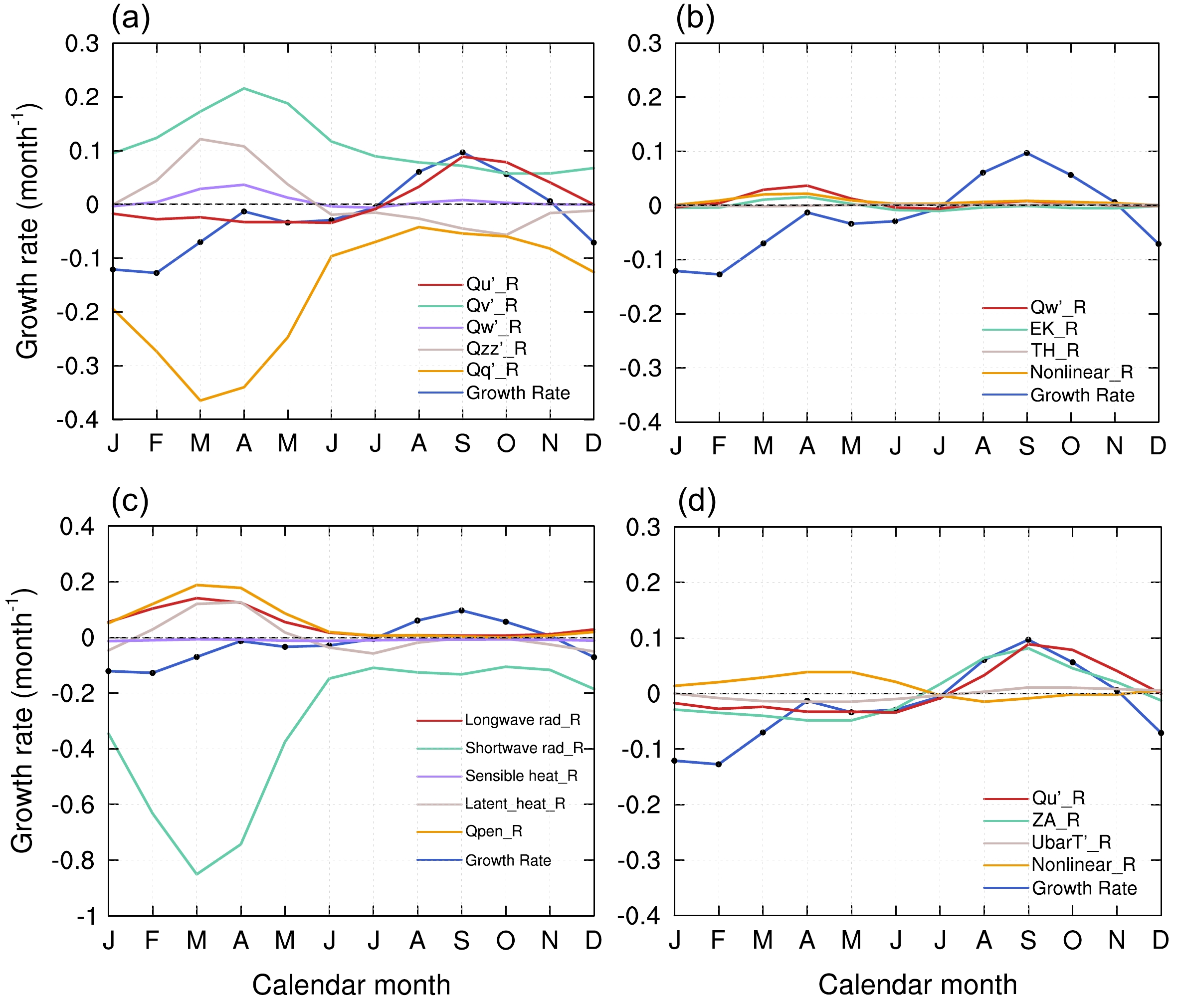
$ T'_t\_R $ , (b) the anomalous dynamic and thermodynamic processes with a variable MLD$ {F'}({\text{varying MLD}})\_R $ , and (c) the anomalous dynamic and thermodynamic forcing terms with a fixed MLD$ {F'}({\text{fixed MLD}})\_R $ (units: month–1). Blue shading indicates the 95% confidence interval in (a) and the 80% confidence interval in (b) and (c). A 3-month running mean has been applied to the plots.Subsequently, as the forcing term in Eq. (4) is composed of five processes, the contribution of each term to the growth rate can be obtained (Fig. 6a). Taking
$ Q'_u $ as an example, the corresponding contribution of$ Q'_u\_R $ can be measured through linear regression by replacing$ {F'} $ in Eq. (5). As shown in Fig. 6a, the contribution calculated by$ Q'_v $ ($ Q'_q $ ) is always positive (negative) throughout the year. The variation of$ Q'_{zz} \_R $ is opposite to the growth rate indicating that$ Q'_{zz} $ essentially makes a negative contribution and that the magnitude of$ Q'_w\_R $ is the smallest among the five terms. Meanwhile, it is not hard to tell that$ Q'_u \_R $ is the closest to the growth rate in terms of its amplitude and variation trend.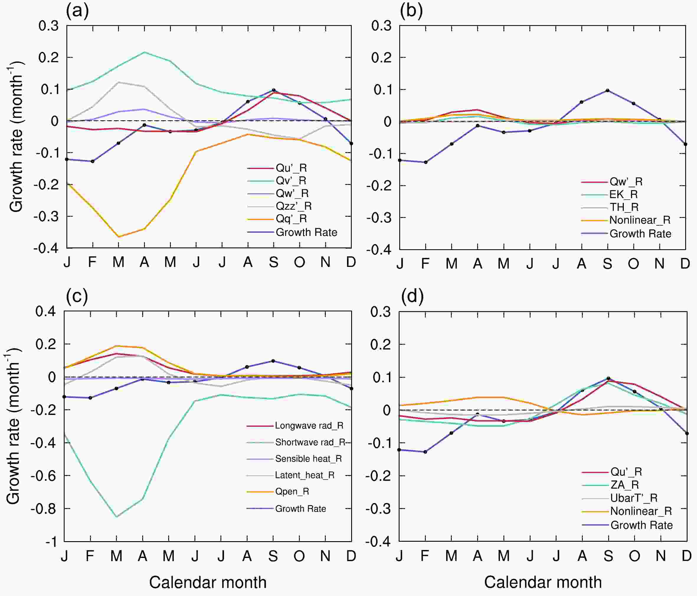
Figure 6. (a) The SST growth rates diagnosed from the anomalous forcing term
$ {F'} $ (Growth Rate, blue curve with dots) with its decomposition into$ Q'_u $ ($ Q'_u\_R $ , red curve),$ Q'_v $ ($ Q'_v\_R $ , green curve),$ Q'_w $ ($ Q_w'\_R $ , purple curve),$ Q'_{zz} $ ($ Q'_{zz}\_R $ , grey curve), and$ Q'_q $ ($ Q'_q \_R $ , orange curve). (b)$ Q'_w $ ($ Q'_w \_R $ , red curve) with its decomposition, EK ($ {\text{EK}}\_R $ , green curve), TH ($ {\text{TH\_}}R $ , grey curve), and nonlinear processes ($ {\text{Nonlinear}}\_R $ , orange curve). (c) Decomposition of$ Q'_q $ , longwave radiation ($ {\text{Longwave rad}}\_R $ , red curve), shortwave radiation ($ {\text{Shortwave rad}}\_R $ , green curve), sensible heat ($ {\text{Sensible heat}}\_R $ , purple curve), latent heat ($ {\text{Latent heat}}\_R $ , grey curve), and penetrative shortwave radiation ($ Q'_{pen} \_R $ , orange curve). (d)$ Q'_u $ ($ Q'_u\_R $ , red curve) with its decomposition, ZA ($ {\text{ZA}}\_R $ , green curve),$ - \overline {{u_a}} {{\partial T'_a }}/{{\partial x}} $ ($ - \overline u {T'}\_R $ , grey curve), and nonlinear term ($ {\text{Nonlinear}}\_R $ , orange curve). A 3-month running mean has been applied in each diagnosing process.As can be readily seen, the development of
$ Q'_v\_R $ and$ Q'_{zz} \_R $ are quite similar, with both of their processes characterized by initial growth and subsequent decay. On the contrary,$ Q'_u\_R $ and$ Q'_q\_R $ resemble a seasonal trend of first rising and then decreasing. From December to July, the contribution of$ Q'_q $ is evidently greater than that of$ Q'_u $ during the negative SST growth rate. In the period characterized by the positive development of growth rates,$ Q'_v $ and$ Q'_u $ are roughly comparable between August and November. Quantitatively, the primary and secondary contributions to the seasonal cycle of growth rate in each calendar month are outlined in Table 1.Jan Feb Mar Apr May Jun Jul Aug Sep Oct Nov Dec Primary $ Q_q' $ $ Q_q' $ $ Q_q' $ $ Q_q' $ $ Q_q' $ $ Q_q' $ $ Q_q' $ $ Q_v' $ $ Q_u' $ $ Q_u' $ $ Q_v' $ $ Q_q' $ Secondary $ Q_u' $ $ Q_u' $ $ Q_u' $ $ Q_u' $ $ Q_u' $ $ Q_u' $ $ Q_{zz}' $ $ Q_u' $ $ Q_v' $ $ Q_v' $ $ Q_u' $ $ Q_{zz}' $ Table 1. The primary and secondary contributions of forcing terms in each calendar month for the seasonal cycle of SST growth rate.
-
We have learned that the contribution of
$ Q'_w $ displays the smallest amplitude among the five feedback processes; however, it contains two important vertical dynamic processes: the thermocline and Ekman feedback. It is possible that contributions from these processes largely offset each other, resulting in the small magnitude of$ Q'_w\_R $ . The influence of both processes upon growth rate is dissected in the following discussion. Decomposition from$ Q'_w $ consists of three components (Fig. 6b), namely the thermocline feedback (TH), Ekman feedback (EK), and nonlinear processes. It is easy to tell that amplitudes of all these terms are fairly small and that the contributions from both EK and the nonlinear term impact the development of the growth rate only slightly between February to May. Besides, these results rule out the speculation of these two vertical dynamic terms offsetting each other as previously conjectured.In quantifying the contribution in Eq. (7), it is clear that
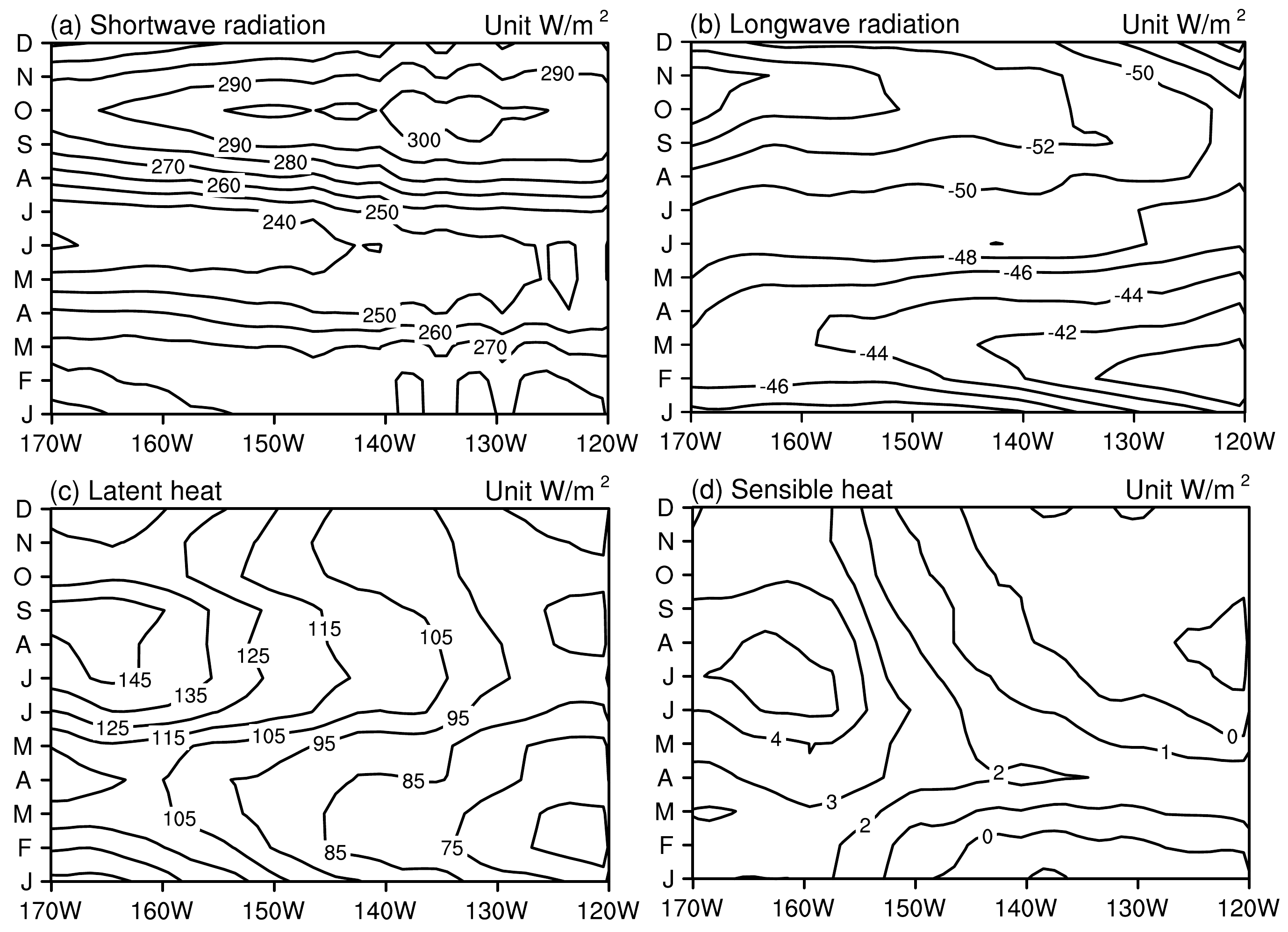
$ Q'_q $ occupies a prominent position in the phase where the growth rate is negative. To analyze the influence of this thermodynamic process, the decomposition of$ Q'_q $ is examined. As shown in Fig. 6c,$ Q'_q $ includes five components, namely shortwave radiation, longwave radiation, latent heat, sensible heat, and shortwave radiation penetrating through the bottom of the mixed layer. It can be observed that shortwave radiation accounts for the largest share (Fig. 6c) and shows a characteristic similar to that of$ Q'_q $ , highlighting the significant contribution of solar radiation to the growth rate. There is a remarkable semiannual cycle of shortwave radiation flux (Fig. 7a), with two heating centers corresponding to spring and autumn, which is closely related to the seasonal shift of ITCZ. It is found that$ {\text{Shortwave rad}}\_R $ mainly drives the growth rate during the spring and summer, with its intensity rapidly decaying soon thereafter. This occurs even though more solar radiation is received during autumn in the Niño-3.4 region, and can be understood through the balance that results from the strong cooling attributed to other thermodynamic processes, resulting in a smaller intensity at that time (Fig. 7). Therefore, the contribution of$ Q'_q $ to the growth rate is highlighted in the phase between spring and summer.
Figure 7. Heat fluxes in the equatorial Pacific (0°) for (a) downward shortwave radiation, (b) downward longwave radiation, (c) sensible heat, (d) latent heat, and (e) penetrative shortwave radiation during 1981–2020 (units: W m–2). Contour intervals (C.I.) are (a) 10, (b) 2, (c) 10, and (d) 1 W m–2. A 3-month running mean has been applied to the plots.
As mentioned earlier,
$ Q'_u\_R $ is marked to be the optimal metric, either in trend or strength, to approach the growth rate compared to the remaining four items. Therefore, it is important to figure out the basic mechanism by which$ Q'_u $ operates on the growth rate. Through its decomposition,$ Q'_u $ consists chiefly of three components,$ - u'_a({{\partial \overline {{T_a}} }}/{{\partial x}}) $ , which is the ZA,$ - \overline {{u_a}} ({{\partial T'_a}}/{{\partial x}}) $ , and nonlinear processes, and the relative contributions corresponding to each item in$ Q'_u $ are placed in Fig. 6d. It can be seen that$ - \overline u {T'}\_R $ oscillates around zero with the smallest amplitude throughout the year. The contribution obtained from the nonlinear term has an opposite trend to the evolution of$ Q'_u\_R $ , with a negative contribution to the development of the growth rate from January to June, diminishing to practically zero in the latter part of the year. In contrast, ZA accounts for the largest proportion of$ Q'_u $ , which conveys the meaning that ZA plays a dominant role in the seasonal cycle of growth rate. Therefore, the interpretation of the ZA turns out to be key for unraveling the development of the SST growth rate.As indicated by the expression of ZA,
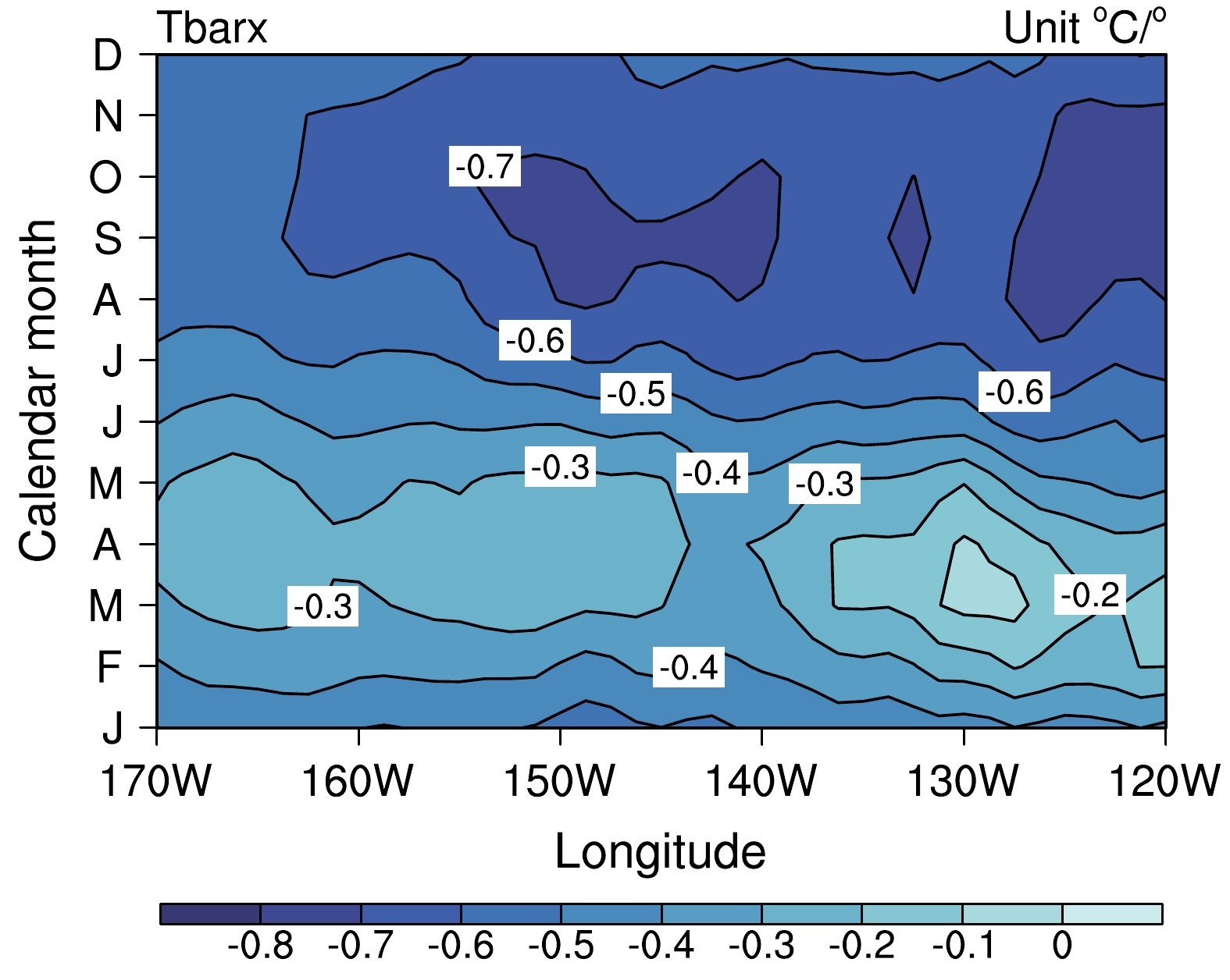
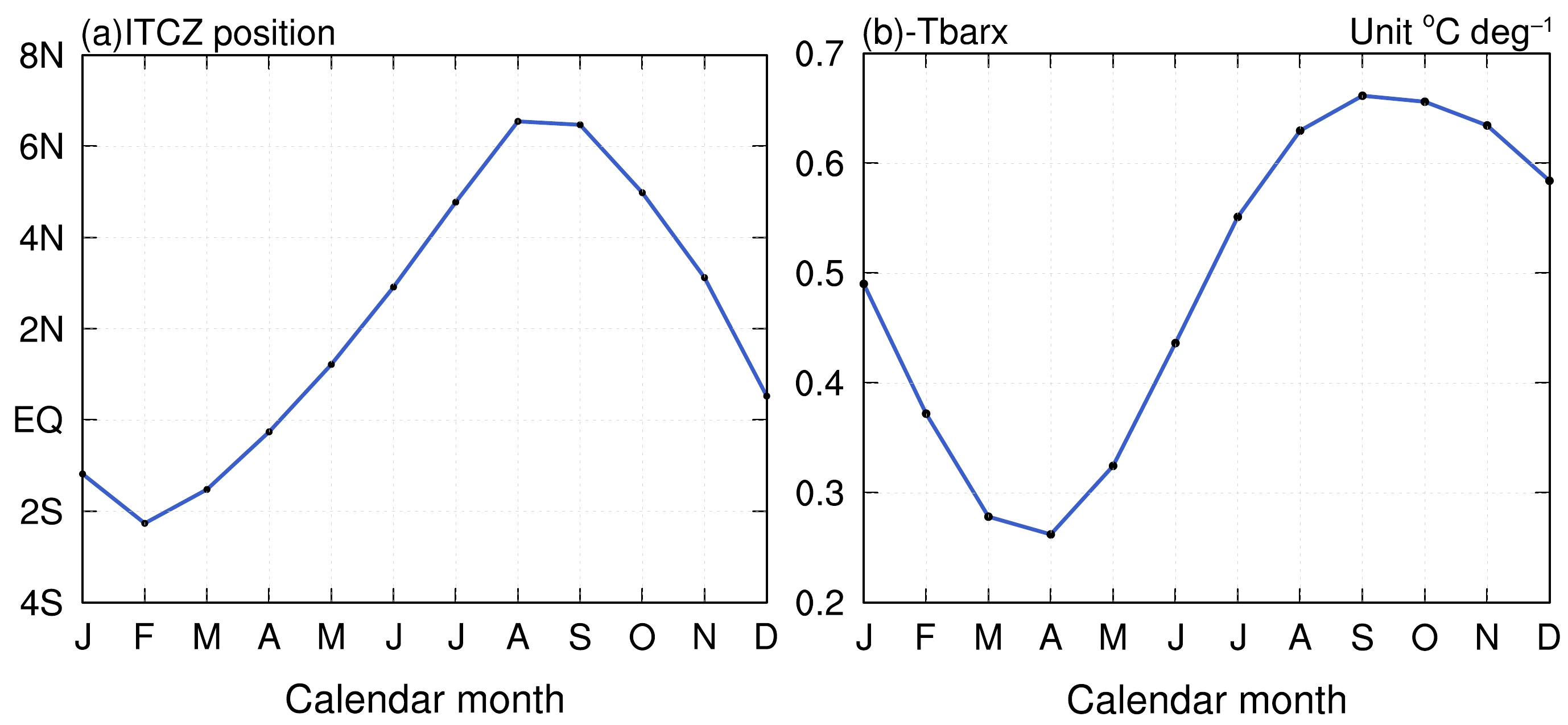
$ \overline {{T_a}} $ , which manifests the variation of the climatic background, determines the strength of this feedback. Figure 8 shows the Hovmöller diagram of$ {{\partial \overline {{T_a}} }}/{{\partial x}} $ ; it can be seen that this parameter is consistently negative for the whole year in the Niño-3.4 region with the maximum and minimum occurring in the boreal spring and near September, respectively. Many studies have revealed that the seasonal variation of SST considerably depends on the meridional migration of ITCZ (Philander, 1983; Xie and Philander, 1994; Tziperman et al., 1997; Xie et al., 2018). As the most characterized seasonal evolution in the tropical Pacific, the ITCZ exerts a large influence on the air-sea coupled system instability. There is a clear correspondence between the seasonal distribution of the ITCZ and its main rainbands as well as the associated warmer SST (Xie et al., 2018; Fang and Xie, 2020). The seasonal variation in Fig. 9a illustrates that the southernmost approach of the ITCZ is near 2°S in February while it marches northward to its farthest extent from the equator in boreal autumn. It is worth noting that the correlation between the seasonal evolution of ITCZ and SST growth rate is markedly significant, both of which present a minimum in boreal spring and a maximum occurring around September, suggesting that the SST growth rate variation is markedly controlled by the seasonal migration of ITCZ.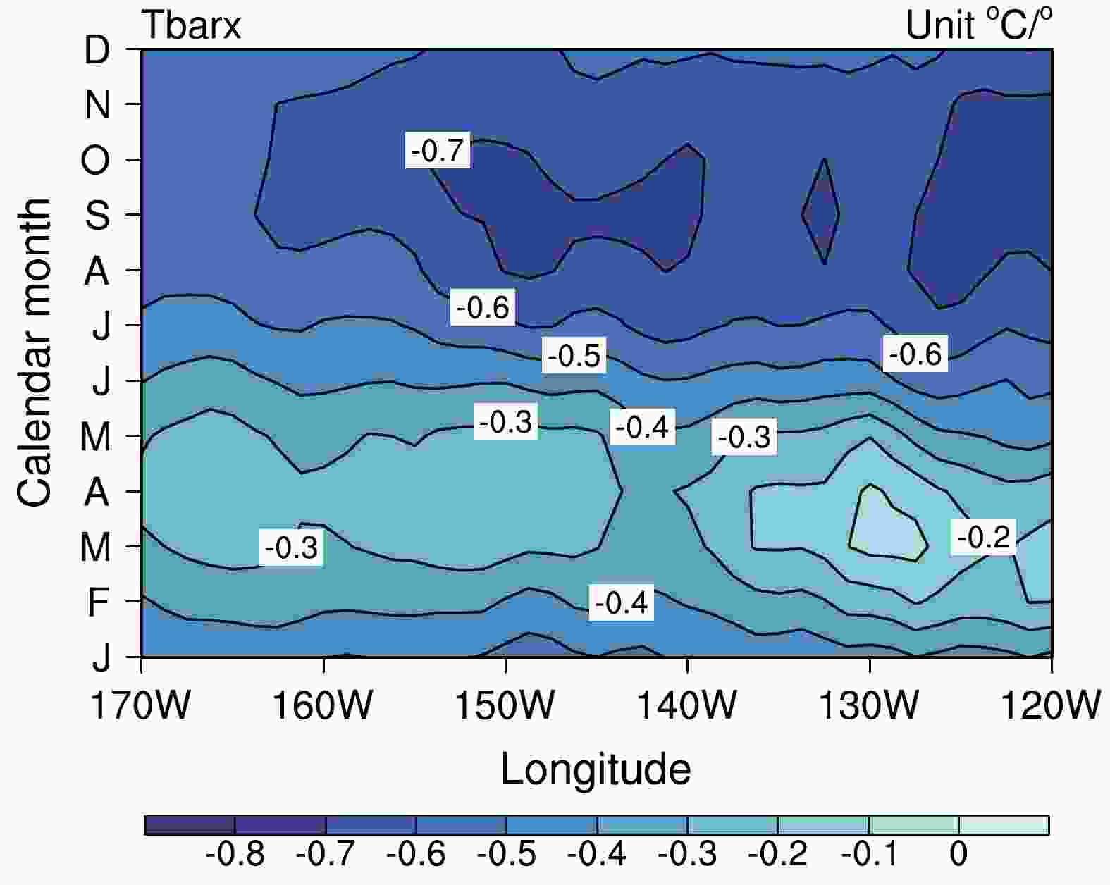
Figure 8. The Hovmöller diagram of
$ {{\partial \overline {{T_a}} }}/{{\partial x}} $ (units: °C deg–1) averaged between 5°N–5°S from 1981 to 2020. The contour interval is 0.1°C deg–1 for$ {{\partial \overline {{T_a}} }}/{{\partial x}} $ . A 3-month running mean has been applied to the plot.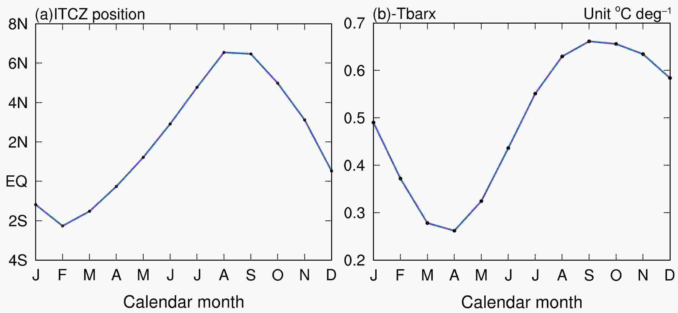
Figure 9. (a) Seasonal immigration of ITCZ in the central to eastern Pacific (170°–120°W) during 1981–2020. (b) Seasonal evolution of
$ - {{\partial \overline {{T_a}} }}/{{\partial x}} $ in the Niño-3.4 region during 1981–2020 (units: °C deg–1). A 3-month running mean has been applied to both of the plots.A brief explanation of mechanisms that potentially affect the modulation of
$ {{\partial \overline {{T_a}} }}/{{\partial x}} $ by the ITCZ follows. As the most salient seasonal movement in the tropical region, the ITCZ is at its southernmost extent in the spring and is accompanied by weak trade winds and westward currents, resulting in the accumulation of more warm water volume to the east tending to maximize around the eastern Pacific. As its location marches gradually northward, the land placed north of the equator becomes a strong heat source related to geographic asymmetries in the tropical Pacific, which leads to strengthening the trans-equatorial flow and southeastward wind resulting in additional warm water transport to the west. Soon afterward, the ITCZ stretches over 6°N in the autumn with a perfectly set up cold tongue near the central to eastern Pacific through several effects including the intense southeasterly trade winds, oceanic evaporation, and latent heat release caused by the wind-driven surface currents and upwelling. Although the received solar shortwave radiation is enhanced along the eastern tropical region during the autumnal equinox, Liu et al. (2005) indicated that the contributions of those cooling processes are far greater than the heating effects from the radiation. It follows that when these factors are coupled together they readily bring the coolest SST during the annual cycle. With the movement of the subsolar point, the ITCZ shifts equatorward causing the eastern Pacific warm again. Accordingly, the tropical Pacific background state repeatedly circulates and is governed by the seasonal migration of ITCZ. This process is of great importance for the SST variation and ZA which plays a dominant role in regulating the seasonal cycle of growth rate. As displayed in Fig. 9b, the seasonal development of ZA has a proximate trend with either the ITCZ or growth rate, all of which tend to be at a minimum during spring before peaking in autumn. However, due to some nonlinear effects, the timing for the minimum of ZA and growth rate do not exactly match, but in general, it can still explain the variation pattern for the seasonal cycle of SST growth rate. -
To reveal the seasonal cycle of the SST growth rate, we adopt the oceanic mixed layer heat budget equation in combination with a recharge discharge model to diagnose the Niño-3.4 region. Note that, different from previous studies that defined the MLD to be a certain value, our results have indicated that the variation of MLD is an important factor that facilitates an accurate understanding of the authentic situation of ENSO as well as portraying the variable characteristic of the growth rate, for omitting the effects of MLD variations can result in potential biases and less robust conclusions.
Growth rates of both
$ T'_t\_R $ and$ {F'}({\text{varying MLD}})\_R $ peak in September, with the negative minimums of those occurring in the boreal spring. On the other hand, the seasonal cycle of${F'}({\text{fixed MLD}})\_R$ still tends to be the strongest during the boreal autumn, but its weakest growth rate is shifted from May to February. This justifies that it is of great importance to consider the variation of MLD when diagnosing the SST growth rate. Subsequently, the contribution of each forcing term to the growth rate are accordingly obtained after decomposition. The contribution as calculated from$ Q'_v $ ($ Q'_q $ ) is always positive (negative) throughout the year. The variation of$ Q'_{zz}\_R $ is opposite to the growth rate indicating that$ Q'_{zz} $ contributes negatively and the magnitude of$ Q'_w\_R $ seems to be the smallest among the five terms. It is also seen that$ Q'_u\_R $ proceeds at a similar pace with the growth rate either in amplitude or variation trend. As can be readily seen, the seasonal evolution of$ Q'_v\_R $ and$ Q'_{zz}\_R $ are quite similar, as their development is characterized by growth at first before decaying. On the contrary,$ Q'_u\_R $ and$ Q'_q\_R $ demonstrate a seasonal trend of an increase followed by a decrease. From December to July, the contribution of$ Q'_q $ is much greater than that of$ Q'_u $ during the negative growth rate period. Coincident with the period exhibiting a positive development of growth rate,$ Q'_v $ and$ Q'_u $ are obviously comparable from August to November.The contribution from
$ Q_w' $ is fairly small, and both EK and nonlinear processes only slightly impact the development of the growth rate from February to May. Shortwave radiation accounts for the largest share, showing a characteristic similar to that of$ Q_q' $ . Balanced by the strong cooling effect from other thermodynamic processes in the autumn, the contribution of$ Q_q' $ to the growth rate is mainly highlighted in the phase between spring and summer.As mentioned above,
$ Q_u' $ plays a dominant role in the growth rate. Through decomposition, we found that the ZA accounts for the largest proportion in$ Q_u' $ , which is of great importance to the seasonal cycle of growth rate. It is also shown that$ {{\partial \overline {{T_a}} }}/{{\partial x}} $ is negative throughout the year with the maximum occurring in the boreal spring and the minimum in September. Since previous studies have indicated that the seasonal variation of SST noticeably depends on the meridional migration of ITCZ, it is of great importance to figure out the basic mechanism of ITCZ to the SST growth rate. As the most characterized seasonal evolution in the tropical Pacific, the ITCZ approaches its southernmost extent in February before it progresses northward to extend farthest from the equator in the boreal autumn. Notably, the seasonal evolution of ITCZ and SST growth rate is markedly significant, suggesting that the SST growth rate and development are visibly controlled by the seasonal migration of ITCZ. In short, the background state in the tropical Pacific circulates repeatedly governed by the seasonal migration of ITCZ and is of great importance for the SST variation. Since ZA is subject to the regulation of ITCZ, it dominates the seasonal variation of growth rate. However, the timing of the minimum ZA and growth rate do not exactly match due to some nonlinear effects, but it can still explain the variation pattern for the seasonal cycle of the SST growth rate in general. This differs from the conclusions of Chen and Jin (2021) who preferred to appreciate both the ZA and TH. To elucidate, the geostrophic flow links the zonal current to the depth of the thermocline and the influence of zonal current has been summarized to the vertical direction. The contribution of ZA seems to be greater through our diagnosis. This paper emphasizes the importance of ZA and provides a possible conceptual direction for the improvement of the model.Acknowledgments. This work is supported by the National Natural Science Foundation of China (Grant No. 42192564), Guangdong Major Project of Basic and Applied Basic Research (Grant No. 2020B0301030004), and the Ministry of Science and Technology of the People's Republic of China (Grant No. 2020YFA0608802).
-
As mentioned by Huang et al. (2010), the mixed layer temperature heat budgets can be described as
where F consists of five terms, zonal advection [
$ {Q_u} = - {u_a}({{\partial {T_a}}}/{{\partial x}}) $ ], meridional advection [$ {Q_v} = - {v_a} ({{\partial {T_a}}}/ {{\partial y}}) $ ], vertical entrainment [$ {Q_w} = - w({{\partial {T_a} - \partial {T_{{\text{MLD}}}}}})/{{\partial z}} $ ], vertical diffusion [$ {Q_{zz}} = - ({{{\mathrm{Ec}}}}/{{{\text{MLD}}}})({{\partial {T_a} - \partial {T_{{\text{MLD}}}}}})/{{\partial z}} $ ], and adjusted surface heat flux caused by radiation ($ {Q_q} $ ). Variables with the subscript a denote the vertical average from the sea surface to the mixed layer bottom, and the subscript MLD is the mixed layer depth. The subscript MLD indicates a certain value of the variable at the bottom of the mixed layer.$ T $ ,$ u $ , and$ v $ represent the temperature and horizontal ocean currents. Since the vertical processes of$ {Q_w} $ and$ {Q_{zz}} $ are difficult to capture and treated as residual terms at some point, these can be characterized through parameterization. Here,$ w $ in$ {Q_w} $ is derived from:Other than that,
$ {\mathrm{Ec}} $ is calculated by:where Ri in Eq. (A4) is the Richardson number described as:
note that Ri is confined with the minimum value of –0.1, to ensure a rational diagnosis.
$ \lambda $ in Eq. (A4) and$ \delta $ Eq. (A5) are given by:and
respectively.
The last term
$ {Q_q} $ is defined asin which
$ {Q_t} $ is the total downward heat flux,$ {Q_s} $ represents the shortwave radiation, and$ \rho $ and$ {c_p} $ are the water density and heat capacity, respectively.The constant parameters from Eq. (A4) to (A8) are summarized in Table A1. Simple physical interpretations and specific algorithms of each dynamic and thermodynamic process are displayed in Table A2 as well.
Parameters Values $ {E_z} $ 1 × 10⁻⁵ $ {{\text{m}}^{\text{2}}}{\text{ }}{{\text{s}}^{{{ - 1}}}} $ $ \alpha $ 5 $ g $ 9.8 $ {\text{m }}{{\text{s}}^{{{ - 2}}}} $ $ \varepsilon $ 8.75 × 10⁻⁶ $ \rho $ 103 kg m–3 $ {c_p} $ 4.2 × 10³ J kg–1 °C $ {\lambda _0} $ 1 × 10⁻⁴ $ {{\text{m}}^{\text{2}}}{\text{ }}{{\text{s}}^{{{ - 1}}}} $ $ {\lambda _1} $ 3.5 × 10⁻³ $ {{\text{m}}^{\text{2}}}{\text{ }}{{\text{s}}^{{{ - 1}}}} $ Table A1. Constant parameters and corresponding values from Eqs. (A4) to (A8).
Term Physical interpretation Specific algorithm $ {Q_u} $ zonal advection $ - {u_a}({{\partial {T_a}}}/{{\partial x}}) $ $ {Q_v} $ meridional advection $ - {v_a}({{\partial {T_a}}}/{{\partial y}}) $ $ {Q_w} $ vertical entrainment $ - w({{\partial {T_a} - \partial {T_{{\text{MLD}}}}}})/{{\partial z}} $ $ {Q_{zz}} $ vertical diffusion $ - ({Ec}/{{\text{MLD}}})({\partial {T_a} - \partial {T_{{\text{MLD}}}}})/{{\partial z}} $ $ {Q_q} $ adjusted heat flux by radiation $ {Q_t} - {Q_s}(0.58{e^{\frac{{ - {\text{MLD}}}}{{0.35}}}} + 0.42{e^{\frac{{ - {\text{MLD}}}}{{23}}}})/\rho {c_p}{\text{MLD}} $ $ {T_t} $ temperature tendency $ {{\partial {T_a}}}/{{\partial t}} $ TH thermocline feedback $ - \overline w ({{\partial T_a' - \partial T_{{\text{MLD}}}'}})/{{\partial z}} $ EK Ekman feedback $ - {w'}({{\partial{ \overline {T_a'}} - \partial \overline {T_{{\text{MLD}}}'} }})/{{\partial z}} $ ZA zonal advective feedback $ - u_a' ({{\partial \overline {{T_a}} }}/{{\partial x}} )$ Table A2. Simple physical interpretations and specific algorithms of each dynamic and thermodynamic process.
Eq. (A2) is written by removing the climatology in each term as follows:
where the Eddy term has been neglected.
Here,
and
In addition,
and
| Jan | Feb | Mar | Apr | May | Jun | Jul | Aug | Sep | Oct | Nov | Dec | |
| Primary | $ Q_q' $ | $ Q_q' $ | $ Q_q' $ | $ Q_q' $ | $ Q_q' $ | $ Q_q' $ | $ Q_q' $ | $ Q_v' $ | $ Q_u' $ | $ Q_u' $ | $ Q_v' $ | $ Q_q' $ |
| Secondary | $ Q_u' $ | $ Q_u' $ | $ Q_u' $ | $ Q_u' $ | $ Q_u' $ | $ Q_u' $ | $ Q_{zz}' $ | $ Q_u' $ | $ Q_v' $ | $ Q_v' $ | $ Q_u' $ | $ Q_{zz}' $ |


 AAS Website
 AAS WeChat