


 DownLoad:


-
The urban heat island (UHI) refers to the phenomenon of higher temperature in a city than in its adjacent rural land. The UHI intensity can be quantified as the urban–rural contrast in surface temperature (SUHI) and in near-surface air temperature (AUHI). Both quantities are city-scale means. The SUHI is measured by thermal sensors on satellites. The same sensors scan the Earth’s surface, providing consistent and repeated sampling of cities across the globe. Generally, the SUHI intensity is computed from the city-wide mean surface temperature and the mean surface temperature of rural pixels in a buffer zone outside the city (Imhoff et al., 2010; Peng et al., 2012). Controls of spatial and temporal patterns in the SUHI are well understood (Zhao et al., 2014; Cao et al., 2016; Li et al., 2019; Manoli et al., 2019). In comparison, our understanding of the AUHI patterns and their controlling factors is still primitive. The intensity of the AUHI is generally quantified with the screen-height air temperature observed at an urban weather station paired with a rural station in its vicinity. Owing to large intracity variations in air temperature, a single station is an inadequate representation of the city-scale mean state (Ziter et al., 2019; Venter et al., 2021; Qian et al., 2022). Furthermore, some urban stations may be situated in urban open greenspaces, and are thus not representative of conditions in built-up areas.
Published studies on the AUHI at the regional and global scales reveal that the AUHI differs from the SUHI in temporal patterns. Over the diurnal cycle, the SUHI peaks during the daytime (Bounoua et al., 2015), but the AUHI is usually greater at night (Oke and Maxwell, 1975; Oke, 1981; Jänicke et al., 2017). In terms of seasonal variations, the SUHI appears stronger in hot and wet seasons (Zhang et al., 2010), while the AUHI is stronger during cold and dry seasons (Adebayo, 1987; Jauregui, 1997; Roth, 2007). Studies that compare the SUHI and the AUHI across climate zones show that the SUHI is stronger than the AUHI by an average of 1.1 ± 1.1 K during the daytime and 0.3 ± 1.5 K during the nighttime (Du et al., 2021). Cities in the arid climate zone appear to be exceptions, where the AUHI is 0.8 K greater than the SUHI during the daytime (Du et al., 2021).
In comparison with the SUHI, the spatial variations in the AUHI and the associated biophysical controls are less understood. The SUHI is generally stronger in wetter climates (Peng et al., 2012; Zhao et al., 2014; Cao et al., 2016; Li et al., 2019; Manoli et al., 2019, 2020). A robust positive relationship exists between annual mean precipitation and the daytime SUHI intensity (Zhao et al., 2014; Manoli et al., 2019). With regard to the spatial gradient in the AUHI, one study showed that the AUHI is negatively correlated with climate wetness (Liu et al., 2020), but another revealed that the AUHI is uncorrelated with precipitation (Du et al., 2021). The divergence between these studies may be caused by site selection uncertainties due to large intracity variations in air temperature.
In this study, we used the data generated by an urban climate model to investigate spatial variations in the AUHI and the underlying climate and ecological drivers. This strategy has been widely used in studies on UHIs as across North America (Zhao et al., 2014), in China (Cao et al., 2016), and globally (Oleson et al., 2011; Zhao et al., 2021). Use of model data instead of weather station observations offers three advantages. First, in the model world, the AUHI is a true city-wide quantity and is not subject to uncertainties associated with intracity microclimate variability. Second, the number of urban clusters is large enough in the model domain, allowing robust statistical analysis. Third, in addition to screen-height temperature, the model provides complete data on all the surface energy balance variables, allowing us to investigate mechanisms underlying the AUHI formation and to perform attribution of the AUHI intensity. A total of 355 urban clusters across China were used, spanning a large climate gradient from subtropical climate in the southeast to semiarid climate in the northwest. Our first objective is to investigate whether the spatial variations in the AUHI are primarily controlled by the background climate (temperature and precipitation) or by background ecological attributes, such as leaf area index (LAI).
Our second objective is to perform attribution analysis of the AUHI intensity. Zhao et al. (2014) carried out quantitative attribution of the SUHI to different drivers (e.g., albedo, convection efficiency, evaporation, anthropogenic heat, heat storage). According to Zhao et al. (2014), convection efficiency explains most of the spatial variations in the SUHI. Here, convection efficiency is inversely proportional to the aerodynamic resistance to heat transfer in the surface layer air. Later, Rigden and Li (2017) presented a revision of this attribution theory by including the surface resistance to water vapor transfer. In the case of AUHI, no equivalent solution exists. The published studies on the AUHI formation are still based on statistical analysis. To our knowledge, the study of Wang and Li (2021) appears to be the only exception. They proposed an attribution method of the AUHI by linking the 2-m air temperature with surface temperature through the assumption of a constant heat flux layer. They tested their method against the AUHI simulated by the Weather Research and Forecasting model in two cities (Boston and Phoenix, USA) during a short heatwave event. Here, we apply a similar methodology, but to the annual mean state and to more than 300 city clusters. In doing so, we hope to elucidate the mechanisms underlying the AUHI formation under different background climates and the AUHI spatial variations across China.
-
The Community Land Model version 5.0 (CLM5.0) is the land component of the Community Earth System Model (CESM) (Danabasoglu et al., 2020). It uses a nested hierarchy consisting of up to five land units (glacier, urban, agricultural, vegetation, and lake) in a grid cell to represent the land surface heterogeneity at the subgrid level (Lawrence et al., 2019a). The vegetation unit is further broken down to plant functional types. In the present study, these plant functional types are regrouped to tree, grass, shrub, and bare soil tiles. The surface fluxes are calculated for each tile at subgrid level, then the area-weighted average is computed at grid level. A full description of the model data is provided by Zhang et al. (2023). A brief summary is given below.
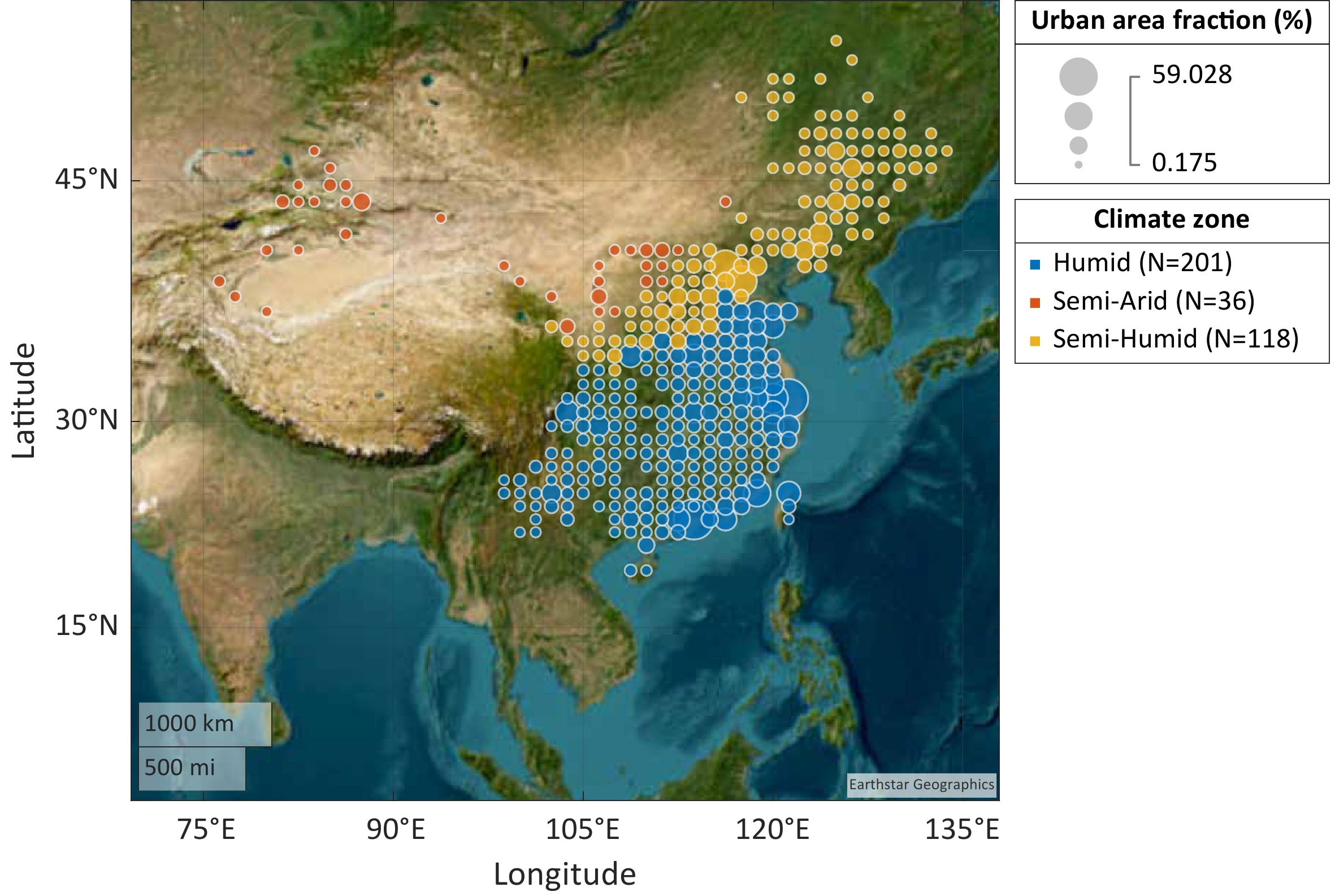
The simulation was conducted at a 0.9°×1.25° resolution under the Representative Concentration Pathway 8.5 (RCP8.5) scenario from 2015 to 2100. There are 355 grid cells containing both urban and rural tiles across China. They fall into three climate zones: humid (201 grids), semi-humid (118 grids), and semi-arid (36 grids) (Fig. 1) according to the Köppen–Geiger climate classification. In CLM5.0, plant phenology is prescribed by satellite observations (Zhang et al., 2023). The surface data were fixed at present-day levels in the simulation, which used the urban land cover in 2020 under the Shared Socioeconomic Pathway 5 (SSP5) scenario from He et al. (2021). Prior to the coupled simulation, a spin-up simulation was conducted offline using GSWP3 (Global Soil Wetness Project phase 3) observation data from 1991 to 2010. The forcing data were cycled for 60 years until the surface climates reached equilibrium [Fig. S3 of Zhang et al. (2023)]. The initial land condition for the spin-up simulation is a default initial file in the year 2011 provided by CESM2. Model outputs are archived for eight land tiles (urban, rural, tree, grass, shrub, bare soil, crop, and lake), including key variables on the physical state, surface energy fluxes, and atmospheric forcing conditions. The urban tile is based on the urban canyon concept, which consists of five components: roof, sunlit wall, shaded wall, pervious canyon floor, and impervious canyon floor. Hourly outputs are available for two periods: 2019–23 and 2096–2100. We only used the variables of urban and rural subgrid tiles at hourly intervals from 2019 to 2023. Unless stated otherwise, our analysis is restricted to midday [1300 LST (local solar time)] and midnight (0100 LST). The two selected times can represent the typical daytime and nighttime conditions according to the AUHI diurnal variations [Fig. S1 in the electronic supplementary material (ESM)]. The broad spatial patterns among the three climate zones are unchanged if longer averaging periods (1200–1600 LST and 0000–0400 LST) are used (Table 1). Also archived are subgrid auxiliary data, including LAI, urban street height-to-width ratio, urban area fraction, and plant functional types.
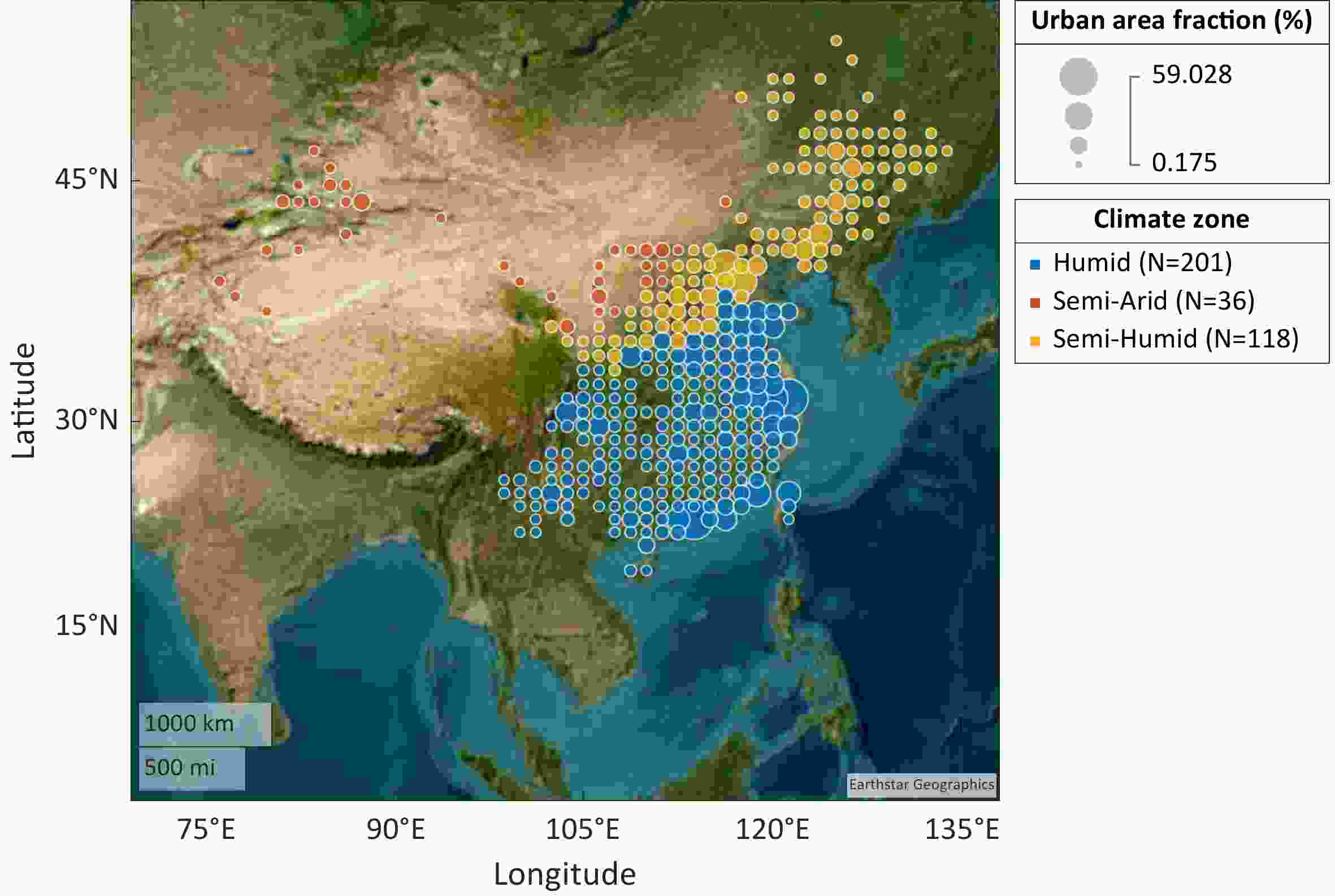
Figure 1. Spatial distribution of urban area fraction in each model grid cell across China.
Averaging period (LST) Humid Semi-humid Semi-arid Daytime 1200–1300 0.34 ± 0.14 0.50 ± 0.14 0.73 ± 0.13 1200–1600 0.46 ± 0.12 0.58 ± 0.10 0.73 ± 0.13 Nighttime 0000–0100 0.75 ± 0.31 0.95 ± 0.31 0.81 ± 0.37 0000–0400 0.71 ± 0.30 0.91 ± 0.30 0.80 ± 0.36 Daily 24-h mean 0.58 ± 0.19 0.75 ± 0.17 0.72 ± 0.23 Table 1. Daytime, nighttime and daily mean AUHI (mean ± one standard deviation; K) for three climate zones across China.
The AUHI is computed as the difference in the screen-height air temperature between the urban tile and the rural tile in the same model grid. The temperature of the rural tile is an area-weighted average of bare soil, crop, tree, grass, and shrub temperatures. In Fig. S2 in the ESM, we show the air temperature of these individual tiles for three grid cells in three different climate zones, corresponding to Nanjing, Beijing and Urumqi, to demonstrate typical within-grid air temperature variations.
-
In our study, the AUHI intensity is quantified as the 2-m air temperature difference between the urban and rural tiles (∆T2) in the same model grid cell. In the following, we describe a diagnostic framework for attributing ∆T2 to different biophysical drivers. The basis of this framework is the analytical solution of surface temperature Ts from the surface energy balance equation (Zhao et al., 2014),
where Tb is air temperature at the blending height,
$R_n^*$ is apparent net radiation, QA is anthropogenic heat flux, Qs is storage heat flux, f is the dimensionless energy redistribution factor, and${\lambda _0}$ is the local climate sensitivity. Qs is calculated as the residual of the surface energy balance equation (Lawrence et al., 2019b). It is the sum of all the heat storage components, including biomass heat storage (Swenson et al., 2019), soil heat storage, and heat storage in canopy air. The anthropogenic heat in CLM5.0 consists of space heating and air conditioning loads to keep the indoor temperature within a comfortable range. Because this parameterization omits vehicle heat release, the anthropogenic heat flux in CLM5.0 is biased low (Zhang et al., 2023). Details of the parameterization are described by Oleson and Feddema (2020). The three intermediate variables are given bywhere σ is the Stefan–Boltzmann constant,
$\varepsilon $ is surface emissivity, K↓ is incoming solar radiation, L↓ is incoming longwave radiation, α is surface albedo, rt is the total resistance for heat transfer between the surface and the blending height, β is the Bowen ratio (ratio of sensible heat flux to latent heat flux), ρ is air density, and Cp is the specific heat of air at constant pressure.On the assumption that sensible heat flux is constant with height between the surface and the blending height, we can relate T2 to Ts as (Wang and Li, 2021)
where R = ra / rt, and ra is the aerodynamic resistance between the 2-m height and the blending height.
Differentiation of Eq. (5) yields a diagnostic equation for the AUHI:
where Δ denotes the urban–rural difference in a variable. The changes in surface roughness and Bowen ratio can cause changes in energy redistribution. Their individual contributions are given by
Terms on the right hand side of Eq. (6) represent contributions from the urban–rural difference in convection efficiency (term 1), evaporation (term 2), radiative forcing (through changes in surface albedo and emissivity, term 3), heat storage (term 4), and anthropogenic heat release (term 5).
In our diagnostic analysis, the blending height is equivalent to the first model grid height (~30 m). The two resistance terms are calculated from the following diagnostic relations:
where H is sensible heat flux. All other variables in Eq. (6) are provided by the model.
To validate the attribution framework, we compared the modeled AUHI with the sum of the component contributions calculated offline according to Eq. (6). The results (Fig. S3) show excellent agreement at midday (r = 0.99, p < 0.001, RMSE = 0.03 K) and acceptable agreement at midnight (r = 0.75, p < 0.001, RMSE = 0.26 K). Expressed as climate zone means, excellent agreement is found for midday, with the absolute errors less than 0.03 K. At midnight, the absolute errors are less than 0.21 K.
-
In this study, three statistical analysis methods were used to determine the main drivers of spatial patterns of the AUHI across China. First, we performed a single-variable correlation analysis to find the correlation coefficients between the midday and midnight AUHI and two types of drivers: (1) six background climate drivers [annual mean air temperature T, annual precipitation P, incoming solar radiation K↓, incoming longwave radiation L↓, net radiation Rn, and vapor pressure deficit (VPD)]; (2) a background ecological driver (rural LAI). All the drivers are provided by the CESM2 outputs. Danabasoglu et al. (2020) evaluated the performance of CEMS2 in simulating historical air temperature and precipitation.
Second, dominance analysis (Budescu, 1993; Azen and Budescu, 2003) was used to determine the relative contribution of each driver to the spatial variations in the AUHI. Prior to this analysis, all the variables were normalized between 0 and 1, with 0 corresponding to the minimum value and 1 to the maximum value. Firstly, a stepwise multi-variable regression was used to screen the predictors. Let us suppose that we have m predictors after this screening. The regression model with all m predictors is the complete model. We can establish other possible regression models with fewer than m predictors (including null). These models are called subset models. There are a total number of 2m − 1 possible subset models. To determine the dominance of predictor X1, we first select models without X1 as a predictor. We then calculate the increase in variance by adding X1 to the selected subset models. This process is repeated for other m − 1 predictors. The relative contribution of X1 is expressed as the ratio of variance increase by X1 to the total variance increase by all m predictors.
Third, a covariance analysis (Zhao et al., 2014) was performed to determine how the main driver obtained with the above two methods interacts with the biophysical contributions to influence the spatial variations in the AUHI. Let Cc, Ce, Cr, Ch and CAH represent contributions from the five biophysical contributions [terms 1 to 5 in Eq. (6)]. Equation (6) can be rewritten as
where e denotes a residual error resulting from nonlinear interactions among the biophysical factors. The spatial covariance of the AUHI and the main driver is equal to the sum of the covariance between each component contribution and the driver:
-
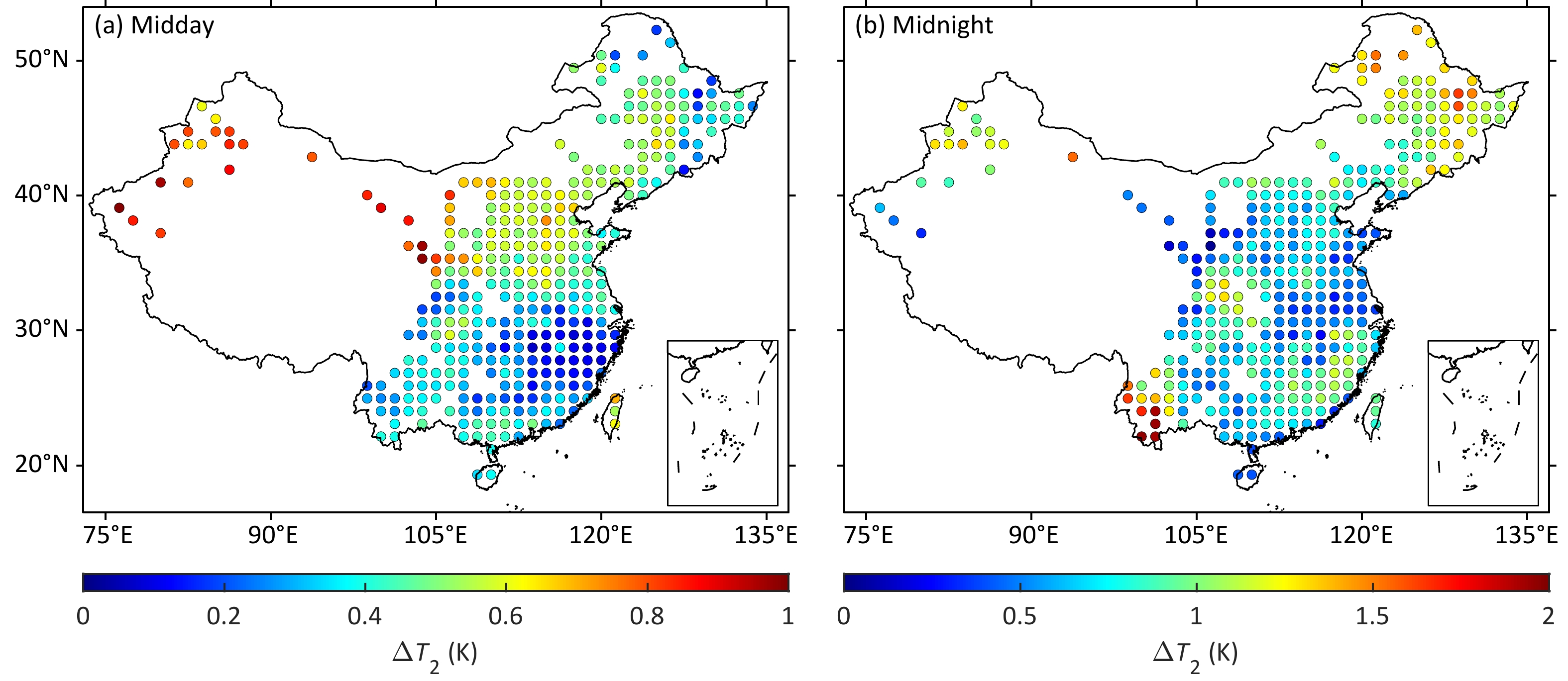
The spatial pattern of the annual mean midday AUHI is opposite to the precipitation gradient across China, being stronger in the semi-arid climate zone than in the humid climate zone (Fig. 2a). The annual mean midday AUHI of the 36 semi-arid cities in Northwest China is 0.73 ± 0.13 K (mean ± one standard deviation), which is 0.39 K greater than that of the 201 humid southern cities (Table 1). The annual mean midnight AUHI does not show a discernible spatial pattern (Fig. 2b). Averaged across the whole country, the midnight AUHI (0.82 ± 0.33 K) is about twice the midday AUHI (0.43 ± 0.19 K).
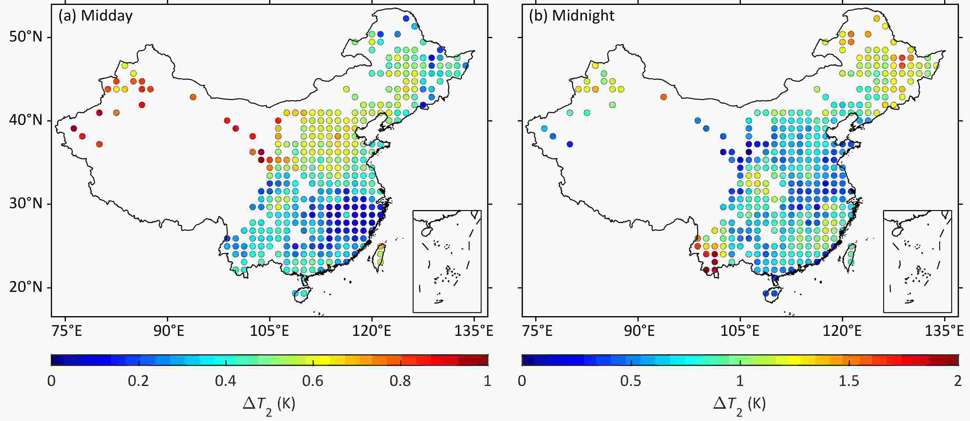
Figure 2. Spatial distribution of the (a) midday and (b) midnight AUHI across China.
The diurnal cycle of the AUHI reported here is in broad agreement with results in the literature. Du et al. (2021) found that 65% of the global cities have a stronger AUHI at night than in the daytime. Their mean AUHI across all the cities was 0.6 ± 1.3 K during the daytime and 0.8 ± 1.4 K during the nighttime. In the review of Arnfield (2003), the nighttime AUHI was generally stronger than the daytime AUHI.
This diurnal pattern is different from that of the SUHI, which is usually greater during the daytime than at night, except for semi-arid cities. The SUHI can be negative for semi-arid cities during the daytime (Zhao et al., 2014). Here, the annual mean AUHI is positive for all the semi-arid cities, both during daytime and at night.
In Fig. 3, we compare our modeled AUHI with the AUHI observed by Li and Zha (2019), Liu et al. (2020), Zhou et al. (2023), Wang et al. (2022), and Peng et al. (2019) for cities in China. In this comparison, the modeled daytime, nighttime, and daily AUHI were calculated as means of the modeled AUHI at the same local times and the same locations as in each of these observational studies. Our modeled daily AUHI agrees well with the observations reported by Peng et al. (2019) and Wang et al. (2022) for the humid and semi-humid climate zones. Although the modeled daily AUHI is slightly lower than the observations for the semi-arid zone, the difference is not statistically significant, with p = 0.08 (independent-samples t-test) when compared with Peng et al. (2019), and p = 0.15 when compared with Wang et al. (2022). The modeled daily AUHI is significantly stronger than the observations reported by Zhou et al. (2023) for the humid and semi-humid climate zones (p < 0.01), and it is nearly identical to the observations for the semi-arid climate zone. The modeled daytime AUHI agrees well with the observations reported by Li and Zha (2019) and Liu et al. (2020) for the humid and semi-humid climate zones, but it is significantly stronger across the three climate zones than that reported by Zhou et al. (2023) (p < 0.01). In the semi-arid climate zone, our modeled daytime AUHI is insignificantly different from the observations reported by Li and Zha (2019) (p = 0.44), and is significantly smaller than that reported by Liu et al. (2020) (p < 0.01). Our modeled nighttime AUHI broadly agrees with the observations reported by Li and Zha (2019) across the three climate zones, but it is lower than the values reported by Liu et al. (2020). There is no significant difference between our modeled nighttime AUHI and the observations reported by Zhou et al. (2023) for the three climate zones (p > 0.42). Overall, the modeled AUHI falls in the range of variations among these five observational studies.
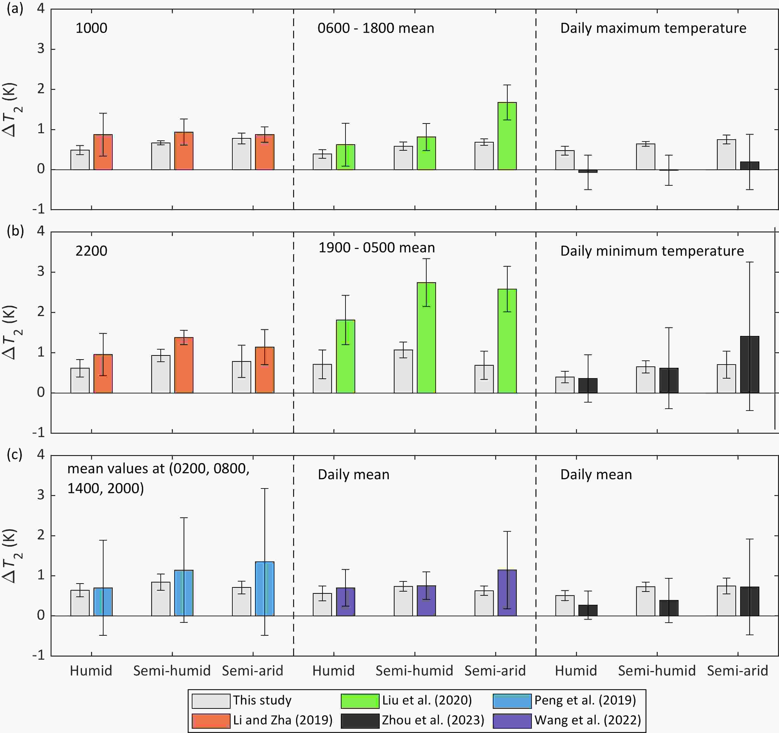
Figure 3. Comparison of the modeled AUHI with observations reported by Li and Zha (2019), Liu et al. (2020), Zhou et al. (2023), Peng et al. (2019) and Wang et al. (2022): (a) daytime; (b) nighttime; and (c) daily. Error bars are one standard deviation of spatial variations.
A number of factors may have contributed to the differences in the modeled and observed AUHI, including underestimation of the anthropogenic heat flux in the model (Zhang et al., 2023), mismatch in the observational [2009 in Li and Zha (2019); 1971–2003 in Liu et al. (2020); 1981–2017 in Zhou et al. (2023); 1984–2023 in Peng et al. (2019); 2019 in Wang et al. (2022)] and modeling time period (2019–23), and uncertainty in the observed AUHI arising from intracity variations in air temperature. These intracity variations may be a reason for why the standard deviation of the observed AUHI is much larger than that of the modeled result, and for why the five observational studies themselves do not agree with each other. An open question is whether the true AUHI can be obtained by a single pair of urban–rural stations and whether urban–rural paired measurements may exaggerate the AUHI intensity (Zhou et al., 2023; Qian et al., 2022). The best strategy to solve the intracity variation problem is to increase the number of observation sites by using high-density networks in the city (Smoliak et al., 2015; Qian et al., 2022). Although the comparison in Fig. 3 indicates that the modeled and observed AUHI agree in order of magnitude, a more comprehensive evaluation of model errors will require dense urban observation networks across the three climate zones.
-
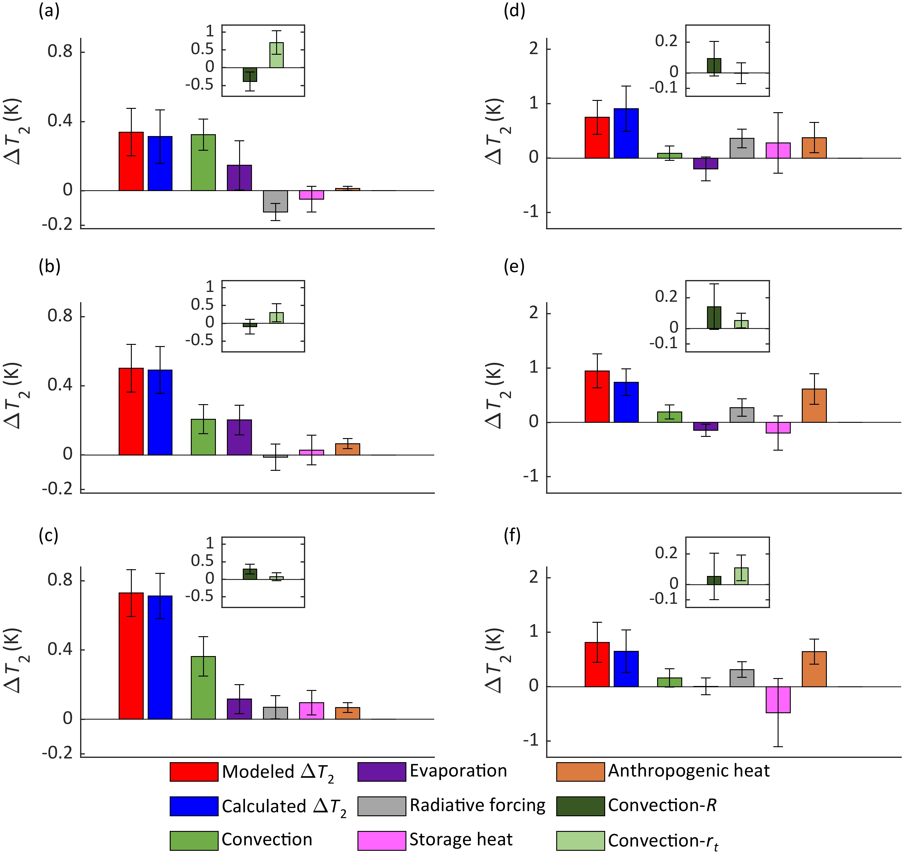
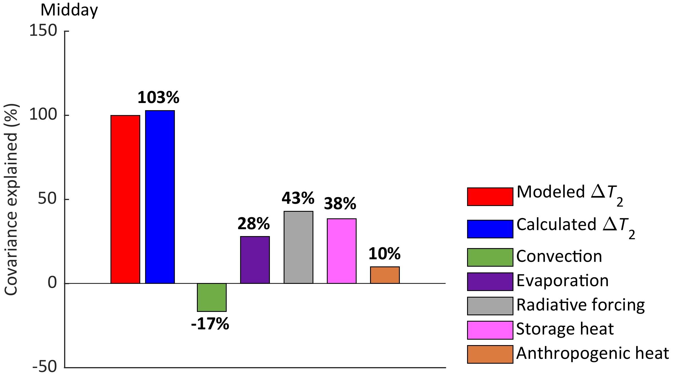
The AUHI is decomposed into five contributions from urban–rural differences in biophysical factors, using the diagnostic framework described in section 2.2 (Fig. 4). Table S1 lists the climate zone means of the variables used for this analysis. Let us first examine the daytime situation. The urban–rural difference in convection efficiency is the largest contributor to the AUHI in the humid (0.32 ± 0.09 K) and the semi-arid (0.36 ± 0.11 K) climate zones (Figs. 4a, c). In the semi-humid climate zone, the contribution from the difference in evaporation (0.21 ± 0.08 K) is close to the contribution from the difference in convection efficiency (0.20 ± 0.09 K) (Fig. 4b). The roles of radiative forcing and heat storage vary across climate zones. Both show negative contributions to the AUHI in the humid climate zone (radiative forcing: −0.12 ± 0.05 K; storage heat: −0.05 ± 0.07 K; Fig. 4a), but positive contributions in the semi-arid climate zone (radiative forcing: 0.07 ± 0.07 K; storage heat: 0.10 ± 0.07 K; Fig. 4b).
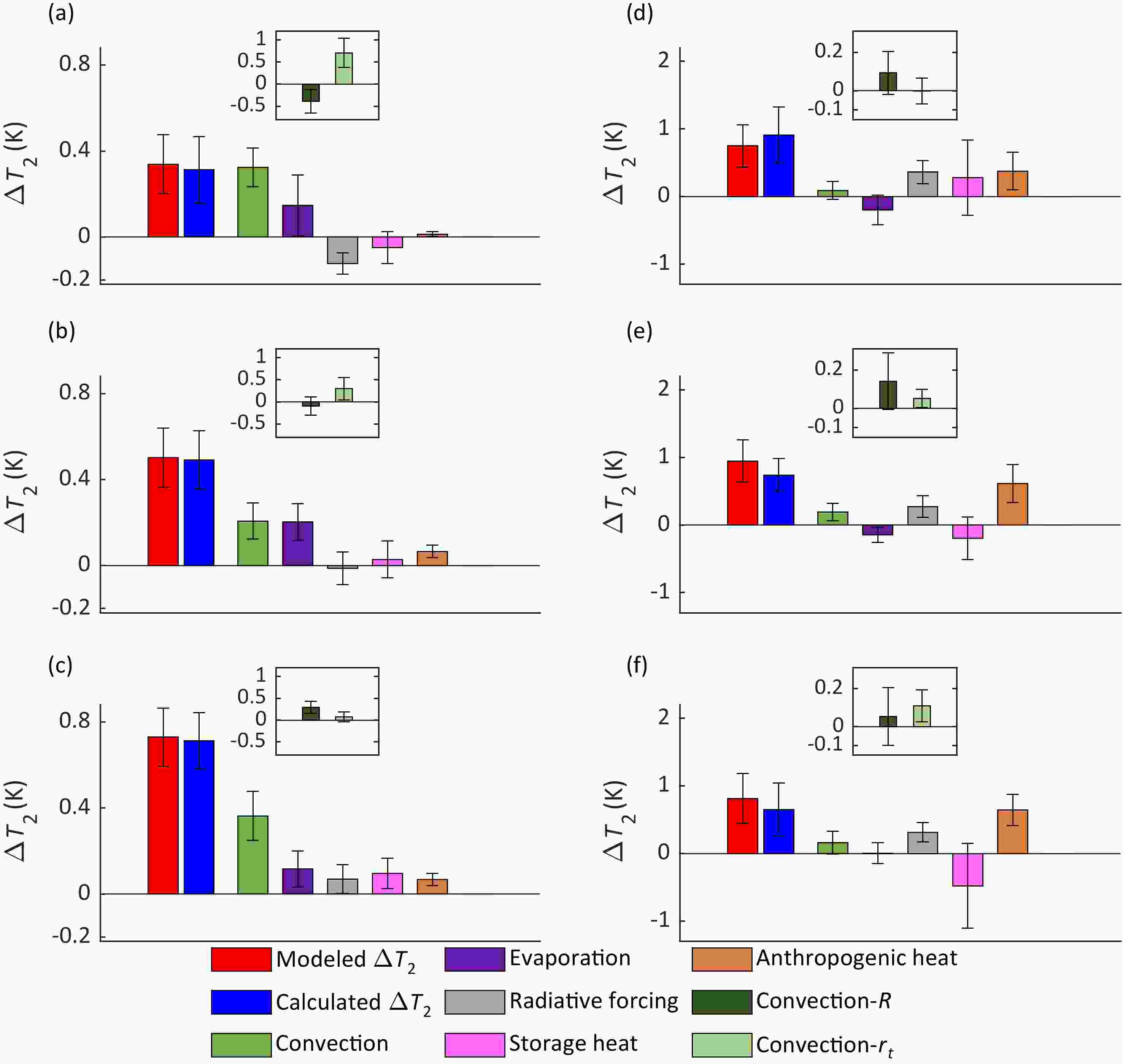
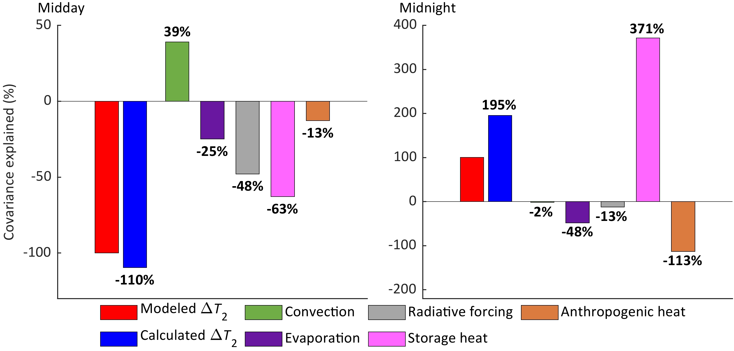
Figure 4. Attribution of the AUHI in three climate zones. The midday AUHI and its component contributions in the (a) humid, (b) semi-humid, and (c) semi-arid climate zone. The midnight AUHI and its component contributions in the (d) humid, (e) semi-humid, and (f) semi-arid climate zone. Red bars denote the modeled AUHI and blue bars denote the AUHI intensity calculated as the sum of component contributions. Error bars denote one standard derivation.
Turning attention now to the nighttime, the release of the anthropogenic heat from urban land is the dominant contributor to the AUHI across the three climate zones. The largest anthropogenic heat contribution occurs in the semi-arid climate zone (0.65 ± 0.23 K; Fig. 4f), due to space heating in the winter. The contributions from storage heat reverses sign from the humid climate (0.28 ± 0.56 K) to the semi-humid (−0.20 ± 0.31 K) and the semi-arid (−0.48 ± 0.63 K) climate zones (Fig. 4d). The rural land with sparse vegetation absorbs more heat than urban areas during the daytime (Table S1 in the ESM). The release of the stored heat during the nighttime warms the rural air more than the urban air. Therefore, the role of heat storage is to reduce the nighttime AUHI in semi-humid and semi-arid climates.
The radiative forcing term [term 3 of Eq. (6)] arises from change in albedo (daytime only) and change in surface emissivity (both daytime and nighttime). Urban land has a smaller emissivity than rural land (Table S1). The result is less longwave radiation loss from urban land and more radiation energy available to warm urban air, which increases the nighttime AUHI (Figs. 4d–f). This positive contribution from the smaller urban emissivity is similar across the three climate zones (0.27 to 0.37 K). During the daytime, the positive contribution from the emissivity difference may be offset by the albedo difference between urban and rural land. Across the three climate zones, the urban–rural difference in emissivity contributes about 0.02 K to the midday AUHI. The average urban albedo is higher than that of rural land in humid and semi-humid climate (Table S1), which decreases the midday AUHI by 0.14 ± 0.05 K for the humid climate zone and 0.03 ± 0.08 K for the semi-humid climate zone. In the semi-arid climate zone, the urban albedo is slightly smaller than that of the rural land, contributing a warming signal of 0.04 ± 0.07 K.
The attribution results for the AUHI are broadly consistent with those reported for the SUHI (Zhao et al., 2014; Cao et al. 2016), but with one exception. In the SUHI attribution, only the total resistance rt is used as the convection efficiency metric. In this study, convection efficiency is measured by a combination of rt and the resistance ratio R. For the same rt, a larger R indicates that heat dissipation is more difficult in the layer from the 2-m height to the blending height, and the 2-m air temperature is higher. In the semi-arid climate zone, the daytime rt of urban land (57 s m−1) is slightly higher than that of rural land (54 s m−1), and the R of urban land (0.17) is also greater than that of rural land (0.14; Table S1). Both factors contribute positively to the AUHI (Fig. 4c). In the humid climate zone, the daytime rt of urban land (70 m s−1) is much larger than that of rural land (37 m s−1), which contributes positively to the AUHI. However, the urban R (0.16) is smaller than the rural R (0.22), which contributes negatively to the AUHI and partially offsets the contribution from changes in rt (Fig. 4a).
The resistance ratio R is related to the surface thermal roughness length. If the surface is smooth, the temperature profile will exhibit a larger vertical gradient near the surface and a smaller gradient above, and we expect a smaller R according to Eq. (5). The temperature profile is logarithmic with height in neutral stability, and the resistance ratio R can be expressed as
where z0,h is thermal roughness length, z2 is the screen height (2 m), and zb is the blending height (~30 m). This equation describes a positive relationship between R and z0,h (Fig. S4 in the ESM).
We also present the attribution results for the summer (Fig. S5 in the ESM) and winter (Fig. S6 in the ESM). During the summer, the urban–rural differences in convection efficiency and evaporation are still the main contributors to the midday AUHI for the three climate zones (Figs. S5a–c). Unlike the annual mean results, the contribution from evaporation is greater than that from convection efficiency for the humid (Fig. S5a) and semi-humid (Fig. S5b) climate zone. At summer midnight, there is no anthropogenic heat contribution, due to the lack of space heating (Figs. S5d–f). During the winter, the urban–rural difference in convection efficiency is the main contributor to the midday AUHI (Figs. S6a–c). The winter midnight result is consistent with the annual result, showing that anthropogenic heat is the main contributor for all three climate zones (Figs. S6d–f).
-
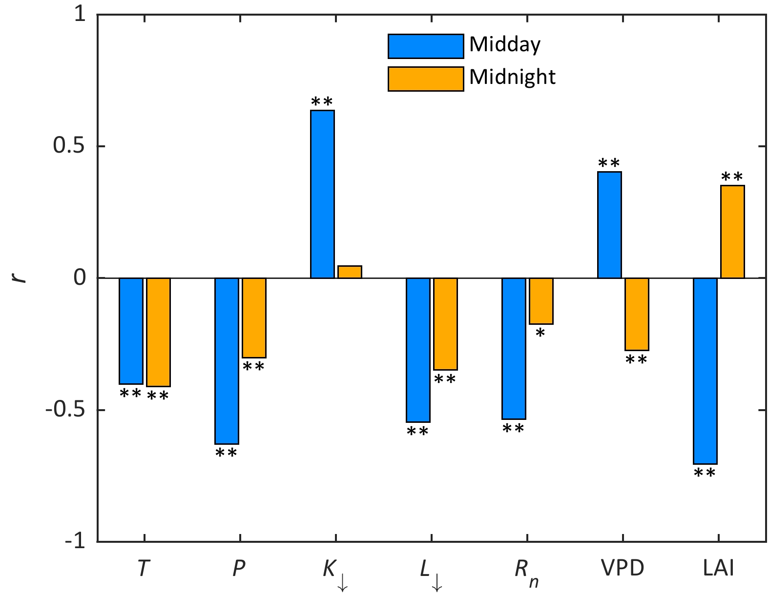
Our single-variable correlation analysis indicates that spatial variations in the midday AUHI are most strongly correlated with the rural LAI (r = −0.71, p < 0.001; Fig. 5). This correlation is negative, meaning that the daytime AUHI decreases with the increasing background vegetation density. The next most influential factor is the incoming solar radiation K↓ (r = 0.64, p < 0.001). A city with higher solar radiation tends to have a stronger midday AUHI. Meanwhile, the daytime AUHI is negatively correlated with the net radiation Rn (r = −0.54, p < 0.001). The seemingly contradictory relationships between the AUHI and K↓ and Rn can be interpreted through the process of longwave radiation feedback. Higher K↓ causes the city surface temperature to be higher, which in turn increases outgoing longwave radiation and decreases Rn.
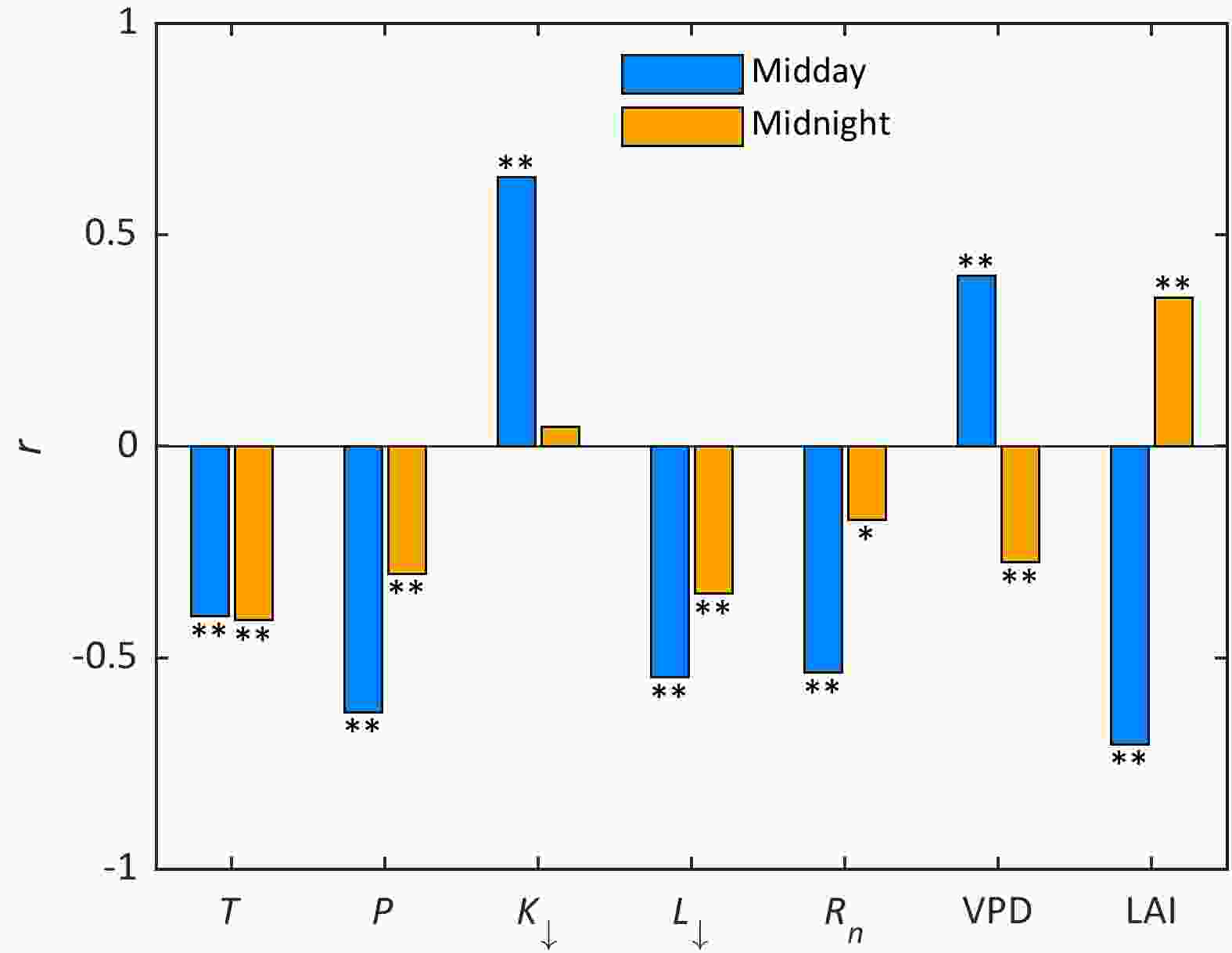
Figure 5. Correlation coefficients between the annual mean midday and midnight AUHI and background drivers. T, annual mean temperature; P, annual mean precipitation; K↓, incoming solar radiation; L↓, incoming longwave radiation; Rn, net radiation; VPD, vapor pressure deficit; LAI, rural leaf area index. * and ** represent significance at the p < 0.01 and p < 0.001 confidence level, respectively.
Generally, the midnight AUHI shows weaker correlations with LAI and the background climate drivers than the midday AUHI, consistent with the lack of spatial coherence shown in Fig. 2b. The strongest negative correlation is found with temperature T (r = −0.41, p < 0.001), and the strongest positive correlation is found with LAI (r = 0.35, p < 0.001).
In the stepwise multi-variable regression, only precipitation, temperature, incoming shortwave radiation, net radiation, and LAI remain as predictors of the midday AUHI. The regression equation is
where the subscript “n” denotes “normalized value”. The dominance analysis revealed that LAI and K↓ have the largest (29%) and second largest (28%) relative importance for ∆T2, respectively (Fig. S7). The relative importance for other predictors is 20% for P, 15% for Rn, and 8% for T. This indicates that LAI and K↓ are the main controlling drivers of spatial variations in the daytime AUHI.
The same stepwise multi-variable regression yields the following equation for the nighttime AUHI:
Once again, LAI is the dominant driver of the spatial variation in the nighttime AUHI, with relative importance of 55% (Fig. S7 in the ESM). The relative importance for other predictors is 16% for T, 16% for L↓ 11% for P, and 2% for K↓.
Correlation coefficients between the AUHI and background drivers have seasonal variations. LAI is still the main driver of spatial variations in the summer midday AUHI (Fig. S8a in the ESM). Unlike the annual mean results, the incoming longwave radiation becomes the main driver for both the midday and midnight AUHI during the winter (Fig. S8b).
-
The above correlation and regression results reveal statistical associations of the AUHI spatial variations with environmental conditions. To shed light on the underlying mechanisms, we performed spatial covariance analysis with each of the biophysical components of the AUHI.
This analysis was firstly applied to LAI, since LAI is the most important driver of the daytime and nighttime AUHI spatial variations. The covariance analysis results indicate that LAI influences the spatial patterns of the AUHI mainly through its regulation of heat storage in rural land (Fig. 6). In the daytime, the overall spatial covariance between the AUHI and LAI is negative, indicating that the AUHI intensity decreases with increasing rural LAI, which is consistent with Fig. 5. Although LAI covaries spatially with all the AUHI biophysical component contributions, its negative covariance with the storage heat contribution is dominant, explaining 63% of the total spatial covariance (Fig. 6a). Indeed, LAI and the heat storage contribution show highly significant and negative linear correlation (r = −0.89, p < 0.001; Fig. S9 in the ESM). Observational studies show that land with sparser vegetation stores and releases more heat during the day and at night, respectively, than land with denser vegetation (Oliver et al., 1987; Wang et al., 2020). A physical interpretation of these spatial covariance results is that if a city is surrounded by a rural landscape with denser vegetation, it is expected to experience a weaker daytime AUHI because less heat is stored in the rural soil and more energy (including heat storage in the canopy) is available to warm the rural surface air. According to the CLM calculation, the rural midday heat storage is 118 W m−2 (positive value indicating heat flux into the soil) when the annual LAI less than 1 (102 cities, mostly in the semi-arid and semi-humid climate zones), and is only 52 W m−2 when the annual LAI greater than 3 (14 cities, mostly in the humid climate zone).
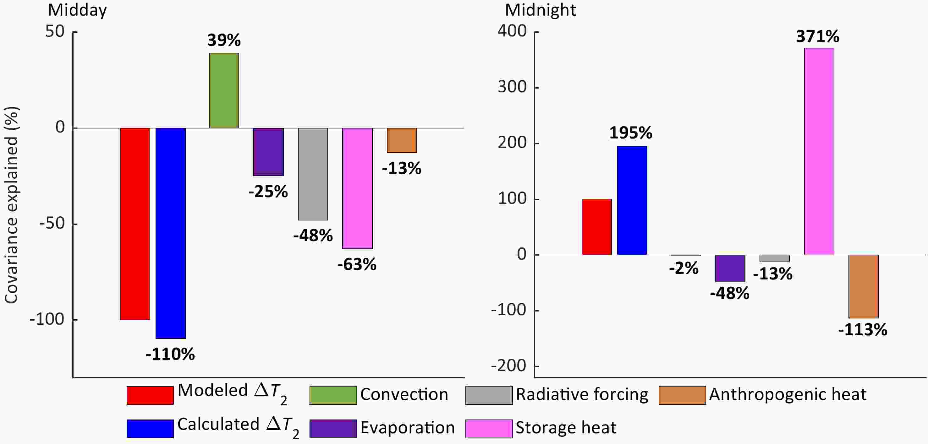
Figure 6. Covariance of rural LAI and different AUHI biophysical factors.
We have shown that the nighttime AUHI is positively correlated with LAI spatially (Fig. 5). The spatial covariance analysis reveals that this positive relationship is dominated by the storage heat contribution covarying with rural LAI (Fig. 6b, Fig. S10 in the ESM). The average rural heat storage term is −24 W m−2 at midnight (negative value indicating that heat is released from the soil) for cities whose rural LAI is greater than 3, and is −62 W m−2 for cities whose rural LAI is less than 1. If a city is surrounded by rural land with denser vegetation, we expect less heat release from the rural soil and biomass at night, a lower rural air temperature, and a greater nighttime AUHI.
The midday AUHI shows a highly significant and positive correlation with the incoming solar radiation K↓ (Fig. 5). The underlying mechanism is complex according to the spatial covariance analysis. This K↓ versus AUHI correlation arises primarily from the influence of K↓ on the radiative forcing contribution to the AUHI, and secondly from its influence on the storage heat contribution (Fig. 7, Fig. S11 in the ESM). For cities with midday K↓ less than 500 W m−2, the midday
$\Delta R_n^*$ is negative (−25 W m−2) and the midday ∆Qs is positive (9 W m−2). These cities with low solar radiation (62 in total) are found mostly in the humid climate zone where the urban albedo (0.19) is higher than the rural albedo (0.12) and where the midday urban heat storage (90 W m−2) is actually higher than the rural land (79 W m−2; Table S1). A negative$\Delta R_n^*$ reduces the AUHI, and so does a positive ∆Qs. For high solar radiation cities (midday K↓ greater than 600 W m−2), the mean$\Delta R_n^*$ is −8 W m−2 and the mean ∆Qs is −5 W m−2. In these cities, which are distributed in three climate zones (18 cities in the humid, 15 cities in the semi-humid, 22 cities in the semi-arid climate zone), radiative forcing and heat storage changes also reduce the AUHI intensity, but by smaller amounts than in low solar radiation cities.
Figure 7. Covariance of incoming solar radiation and different AUHI biophysical factors.
-
We note that there is more than one way to perform diagnostic analysis of the surface temperature response to land use (e. g., Juang et al., 2007; Wang and Li, 2021). Here, it is instructive to compare our method with that used by Wang and Li (2021). In their study, they omitted the anthropogenic heat flux, which may be justifiable because their focus was a short heatwave event. In our study, we find this component to be a large contributor to the annual mean AUHI at night (Fig. 4). Another difference arises from the treatment of surface evaporation. We treated the Bowen ratio as an independent variable and obtained the latent heat flux as the product of the sensible heat flux and Bowen ratio. Wang and Li (2021) used a bulk transfer parameterization with surface resistance to calculate surface evapotranspiration. In their formulation, the latent heat flux is expressed as a function of surface temperature. They considered the AUHI as the sum of 11 contributors. In this respect, their diagnostic framework is more complete than ours. On the other hand, by utilizing the Bowen ratio instead of surface resistance, our method is less prone to outlier influence. This feature is desirable in our efforts to compare multiple cities across a large geographic gradient because too many outliers may introduce biases to such a comparison.
One element common to both approaches is the use of two air resistances to characterize the convection contribution. In this regard, our result is consistent with the study by Wang and Li (2021). They found that, during the daytime, the urban–rural difference in ra is negative for Boston, a city in humid climate, meaning that heat transfer between the 2-m height and the blending height is more efficient over the city than over the adjacent rural land. Their results show that the larger resistance from the 2-m height to the blending height for heat transfer over the rural land with tall trees decreases the daytime AUHI by about 0.5 K. In the present study, the urban resistance ratio R (0.16) is smaller than the rural R (0.22; Table S1), which contributes negatively to the AUHI by about 0.4 K (inset, Fig. 4a). The role of ra is reversed for Phoenix, a city in dry climate, which is a positive contributor to the daytime AUHI. Similarly, in semiarid climate, the R of urban land (0.17) is greater than that of rural land (0.14); this difference is a positive contributor to the daytime AUHI (inset, Fig. 4c).
One limitation of the present modeling framework is its simplistic representation of the urban landscape. It lumps all urban land in a grid cell into a single tile, without distinguishing individual cities within the grid cell. Within the urban tile, only three morphological types (tall building district, high density, and medium density) are allowed. Furthermore, the current version of CLM does not have the capacity to handle urban vegetation. One way to overcome this limitation is to deploy a mesoscale model with urban representation, such as the one used by Wang and Li (2021). Mesoscale models can include detailed prescriptions of soil moisture, greenspace, and intracity variation of building attributes. Generally, mesoscale urban modeling has been restricted to a short duration of a few days to a few weeks and to a few cities, and requires heavy calibration against observations. The computational cost would be prohibitive to run such a model over 5 years and for more than 300 cities, as was done in the present study.
The blending height assumption also deserves attention. The urban and rural tiles in the same model grid are influenced by identical atmospheric conditions specified at the blending height, including air temperature, humidity, incoming solar radiation K↓, and incoming longwave radiation L↓. Strictly, the blending height assumption does not hold for K↓ and L↓. Urban air is more polluted than rural air. Urban aerosols can reduce K↓ in the daytime and increase L↓ both during the day and at night. Although the effect of changes in the incoming radiation on the daytime UHI is negligible due to efficient convection mixing, nighttime changes in L↓ can enhance the UHI intensity (Cao et al., 2016). According to seasonal and annual observations at paired urban and rural sites in Basel, Switzerland (Christen and Vogt, 2004), Beijing, China (Wang et al., 2015), Berlin, Germany (Li et al., 2018), Nanjing, China (Guo et al., 2016) and Montreal, Canada (Bergeron and Strachan, 2012), we estimated that the mean increase of L↓ in urban air relative to the rural reference is +5.4 W m−2. This is roughly the same as the mean midnight anthropogenic heat flux QA in the humid climate and half of the midnight QA in the semi-arid climate (Table S1). According to Fig. 4, the increase of L↓ should contribute to the midnight AUHI by about 0.3°C.
-
In this paper, a global dataset of subgrid land surface climate variables produced by climate model was used to investigate the spatial variations in the AUHI and the underlying climate and ecological drivers across China. Results are presented for individual city clusters as well as mean values for three climate zones (201 cities in the humid, 118 cities in the semi-humid, and 36 cities in the semi-arid climate zone). We found that:
(1) The annual mean midday AUHI is negatively correlated with the precipitation gradient across China. The highest mean AUHI occurs in the semi-arid climate zone (0.73 ± 0.13 K), followed by the semi-humid (0.50 ± 0.14 K) and humid (0.34 ± 0.14 K) climate zones. The annual mean midnight AUHI is stronger than the midday AUHI, but without discernible spatial patterns.
(2) The urban–rural difference in convection efficiency is the largest contributor to the midday AUHI in the humid and semi-arid climate zones, contributing 94% and 49% to the total AUHI, respectively. The release of the anthropogenic heat from urban land is the dominant contributor to the midnight AUHI in all three climate zones.
(3) The rural LAI is the most important driver of the daytime and nighttime AUHI spatial variations. LAI influences the spatial patterns of the AUHI mainly through its regulation of heat storage in rural land.
We caution that these conclusions are based on data generated by an urban climate model. Although the modeled AUHI agrees in magnitude with the observed AUHI in China, the statistical associations with precipitation and LAI need further experimental evaluation. In particular, the connections among the LAI, heat storage, and AUHI spatial distribution should be viewed as a hypothesis requiring independent validation.
Acknowledgements. This research was supported by the National Key R&D Program of China (Grant No. 2019YFA0607202), the National Natural Science Foundation of China (Grant Nos. 42021004 and 42005143). Heng LYU acknowledges support by the Postgraduate Research & Practice Innovation Program of Jiangsu Province (Grant No. KYCX21_0978). Wei WANG acknowledges support by the Open Research Fund Program of the Key Laboratory of Urban Meteorology, China Meteorological Administration (Grant No. LUM-2023-12), and the 333 Project of Jiangsu Province (Grant No. BRA2022023). We thank Long LI, Yan LIU, Decheng ZHOU, Yifan FAN and Shijia PENG for providing the data for Fig. 3.
Electronic supplementary material: Supplementary material is available in the online version of this article at
https://doi.org/10.1007/s00376-023-3012-y .
| Averaging period (LST) | Humid | Semi-humid | Semi-arid | |
| Daytime | 1200–1300 | 0.34 ± 0.14 | 0.50 ± 0.14 | 0.73 ± 0.13 |
| 1200–1600 | 0.46 ± 0.12 | 0.58 ± 0.10 | 0.73 ± 0.13 | |
| Nighttime | 0000–0100 | 0.75 ± 0.31 | 0.95 ± 0.31 | 0.81 ± 0.37 |
| 0000–0400 | 0.71 ± 0.30 | 0.91 ± 0.30 | 0.80 ± 0.36 | |
| Daily | 24-h mean | 0.58 ± 0.19 | 0.75 ± 0.17 | 0.72 ± 0.23 |


 AAS Website
 AAS WeChat