


 DownLoad:


-
The atmospheric system is chaotic; thus, small errors in initial conditions (ICs) can grow rapidly and affect the predictability of Numerical Weather Prediction (NWP) (Lorenz 1965, 1969). Additionally, inaccurate observations and imperfect data assimilation methods cause inevitable errors in ICs. These sources of uncertainty limit the skill and predictability of single deterministic forecasts in NWP. To quantify these initial uncertainties, ensemble prediction systems (EPSs) have been widely applied to represent initial uncertainties in various NWP centers around the world.
It is essential to capture all significant uncertainties as much as possible in ICs with finite ensemble members for a reliable EPS because initial errors are major sources of forecast uncertainties. In addition, multiscale initial errors have different growth behaviors and scale interactions. Specifically, some studies used sophisticated turbulence models to demonstrate that the rapid upscale cascading of small-scale initial errors imposes finite limits on the predictability of mesoscale turbulence (Leith, 1971; Leith and Kraichnan, 1972; Métais and Lesieur, 1986). Also, small- and large-scale errors spread rapidly across all scales, both downscale and upscale (Durran et al., 2013; Durran and Gingrich, 2014; Rotunno et al., 2023). Furthermore, larger-scale initial errors generally lead to greater forecast divergence for heavy-rainfall systems, particularly in cases where the errors are characterized by a preponderance of upward amplification, which can significantly impact the accuracy of the forecast. (Zhang et al., 2007; Durran and Gingrich, 2014; Sun and Zhang, 2016). Meanwhile, the growth characteristics of multiscale initial errors can vary significantly under different conditions, resulting in a flow-dependent predictability skill. (Zhang et al., 2003, 2007; Tan et al., 2004). As a result, it is necessary to comprehensively sample all significant sources of initial uncertainty in the EPS by using reasonable initial perturbation methods to improve prediction skills.
Over the past 30 years, various initial perturbation methods have been developed and applied in different EPSs to represent the initial uncertainty. The singular vectors (SVs) method, which can be regarded as the singular value decomposition (SVD) of an operator (i.e., the so-called forward tangent linear model, TLM) and can physically reflect a collection of the fastest-growing perturbations in dynamical systems (Lacarra and Talagrand, 1988), and represents one of the most widely employed initial perturbation methods. In the 1990s, the European Centre for Medium-Range Weather Forecasts (ECMWF) used SVs to construct the initial perturbations in their Global Ensemble Prediction System (GEPS) (Buizza, 1997; Leutbecher and Palmer, 2008). Subsequently, the SVs method has been widely used in the GEPSs of many other NWP centers, such as Météo-France (Descamps et al., 2015), the Japan Meteorological Agency (JMA) (Yamaguchi et al., 2018), and the China Meteorological Administration (CMA) (Li et al., 2019). Because SVs can capture the most dynamically unstable perturbations, they identify the directions of the initial uncertainty that are responsible for the largest forecast uncertainty (Buizza, 1994a; Buizza and Palmer, 1995; Hoskins et al., 2000; Leutbecher and Palmer, 2008). Hence, SVs are regarded as a very good candidate for producing ensemble members with sufficient spread in the most unstable directions and providing uncertainty information within the probability density function (PDF) of the model state at a given future time (Diaconescu and Laprise, 2012).
Previous studies have shown that different SV structures are associated with distinctive uncertainty information about the atmosphere. Meanwhile, the structure of SVs is sensitive to the energy norm, linearized physical processes, the optimal time interval (OTI), and the choice of TLM horizontal resolution. Buizza (1994b) used a dry total energy (TE) norm with a dry linearized physical process and relatively longer OTI (e.g., 48 h) to calculate dry SVs (including the dry physical process) at a TL63 resolution in a TLM and found that the leading extratropical SVs had a westward tilt at the initial time and a meridional phase tilt that diminished with time. Other studies have used similar settings to calculate SVs and found the same structure as mentioned above (Buizza and Palmer, 1995; Ehrendorfer et al., 1999); moreover, some studies have shown that these SVs can represent the instability of synoptic scale atmospheric baroclinicity in the extratropics (Montani and Thore, 2002; Coutinho et al., 2004). Ono (2021) used moist TE with a moist linearized physical process and relatively shorter OTI (e.g., 6 h) to calculate moist SVs (including the moist physical process) at a 40-km resolution in a TLM and concluded that these SVs can reflect uncertainties in meso-β- to meso-α-scale meteorological systems. Furthermore, increasing the spatial resolution and reducing the OTI to calculate the SVs tends to result in a spatially localized structure, and these SVs can reflect some of meso-β- to meso-α-scale uncertainties which are associated with localized heavy rainfall events (Ehrendorfer et al., 1999; Wang et al., 2020).
Thus, we can see that the traditional single-scale SV initial perturbation approach is unable to comprehensively capture multiscale initial uncertainty information about the atmosphere. To address this issue, Ono (2020) extended the Lanczos algorithm used to produce multiple targeted SV sets in a single computational session to provide more uncertainty information for the EPS. Based on this extension of the Lanczos algorithm, the regional model-based Mesoscale Ensemble Prediction System at the JMA began constructing initial perturbations via a linear combination of SVs with three different spatial and temporal resolutions to capture multiscale uncertainties in the ICs simultaneously (Ono et al., 2021). Ono et al. (2021) found that using multiscale SVs can enhance the probabilistic skill of precipitation forecasts and, in particular, are essential for capturing uncertainties associated with localized heavy rainfall events. Furthermore, Ye et al. (2020) calculated multiscale (i.e., meso-β and meso-α) SVs for generating initial perturbations in the CMA Regional Ensemble Prediction System (CMA-REPS), and the results showed that multiscale SV initial perturbations can reflect more initial uncertainties and improve regional ensemble forecasting skills compared to single-scale SV methods. In conclusion, using multiscale SVs to generate the initial perturbations prove beneficial for the performance of REPSs, but how to optimally design a multiscale SV initial perturbation method for GEPSs remains an open question and is worthy of exploration.
The CMA developed its operational GEPS (i.e., CMA-GEPS) in 2018 (Li et al., 2019; Peng et al., 2022), which used a single-scale SV initial perturbation method to represent the initial uncertainties based on the CMA tangent linear model (TLM) and adjoint model (ADM) (Liu et al., 2018). Recently, Wang et al. (2020, 2023) analyzed the impact of spatial resolutions and physical processes on the structure of SVs based on CMA-GEPS. Their results further suggested that different computational settings result in diverse SV structures which represent distinctive-scale initial uncertainties. All previous research on this topic has served to provide a scientific basis and support to carry out further studies of the multiscale SV initial perturbation method in GEPS.
In this study, a multiscale SV initial perturbation method is developed for capturing multiscale initial uncertainties in CMA-GEPS. To demonstrate how multiscale SVs can affect the initial perturbation characteristics and the ensemble forecast skill, the study also compares the results between multiscale SVs and the single-scale SVs method based on a batch experiment in different seasons. This study aims to develop a multiscale SV initial perturbations method for GEPS, thereby providing a scientific basis for GEPS to be applied more broadly. Following this introduction, section 2 provides details of the multiscale SV initial perturbation method design. Section 3 introduces the CMA-GEPS model and experiment configurations whose results are presented in section 4, Finally, section 5 provides a summary and some further discussion.
-
The fast-growing SVs are calculated by solving an eigenvalue problem defined by the tangent forward and adjoint model. By taking the time evolution of a small perturbation X at an initial time t0 by a tangent forward operator L of the dynamical equations, we obtain:
where X(t) is the evolved perturbation from the initial time t0 to the future time t in the tangent forward model. Equation (1) can be described as a linearized assumption of the nonlinear trajectory of the dynamic systems. Then, the fastest-growing SV is found by identifying the phase–space direction with the largest growth rate J(x) [Eq. (2)] between the evolved perturbation X(t) and initial perturbation X(t0) during the optimal time interval (OTI), so that:
where [.,.] denotes the Euclidean inner product and E is a matrix operator that defines the specific form of the inner product to transform X into a dimensionless vector in Eulerian space, where the expression of the relationship between X and
$ {\mathbf{\hat X}} $ can be represented byIn this study, the dry-TE norm (Liu et al., 2013) is defined by:
where φ denotes the latitude of the spherical coordinate, ρr denotes reference density, Tr denotes reference temperature, θr denotes reference potential temperature, Πr denotes reference dimensionless air pressure, and Cp denotes the specific heat of air at constant pressure. The u and v represent the zonal and meridional wind, respectively,
$\tilde \theta $ ($ \tilde \theta = \theta - {\theta _r} $ ) is the perturbed potential temperature, and$ \tilde \Pi $ ($ \tilde \Pi = \Pi - \Pi_r $ ) is the perturbed Exner pressure corresponding to the perturbations of the CMA-TLM, i.e.,$[{u'},{v'},{(\tilde \theta )'},{(\tilde \Pi )'}]$ [See Liu et al. (2017) for details]. Hence E can be expressed as:As a result, the CMA-TLM perturbed variables with respect to E can be expressed as
$ {\mathbf{\hat X}} $ :Thus, Eq. (2) can be computed as
According to the variational principle of the symmetric matrix, the maximization problem in Eq. (5) can be considered an SVD problem [Eq. (6)]:
where LT is the adjoint model and λ is the eigenvalue of the matrix (ELPE−1)T(ELPE−1). P is the local projection operator (LPO), making it possible to compute SVs in the target area (Buizza, 1994a). Finally, the matrix ELPE−1 is the target SV with the fastest growing rate.
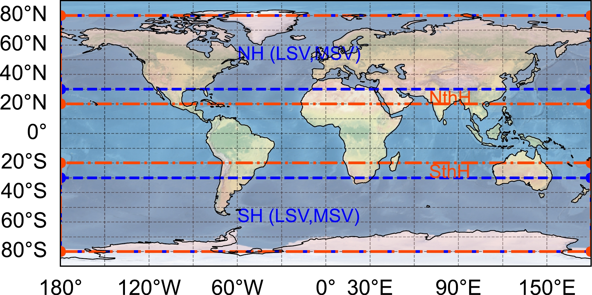
Thus, two types of SVs are computed in this study (The details of these multiscale SVs are summarized in Table 1 and Fig. 1). First, the LSV is designed to represent the synoptic scale uncertainties in the troposphere. The calculation settings for the LSV are the same as the operational GEPS at the CMA. The LSV is computed by 2.5° TLM with dry linearized physical processes (subgrid-scale orographic effect and vertical diffusion), a 48-h OTI, and a dry TE norm. Most NWP centers use similar configurations (e.g., lower horizontal resolution, longer OTI, and a dry-TE norm) to compute an extratropical SV to generate initial perturbation for GEPS (Leutbecher and Palmer, 2008; Descamps et al., 2015; Yamaguchi et al., 2018). Due to the LSV being focused on synoptic scale uncertainties in the troposphere, the dry TE norm is computed by vertical integration from the 4th to 50th model level (nearly 100 m to 16 000 m) over the target areas (NH and SH).
LSV MSV Target area 30°–80°N (NH)
30°–80°S (SH)30°–80°N
30°–80°SResolution 2.5° 1.5° OTI 48 h 24 h Norm Dry TE Dry TE linearized physical processes
(dry)Subgrid–scale orographic effect,
vertical diffusionSubgrid–scale orographic effect,
vertical diffusionNo. of SVs 10 10 Table 1. Calculation settings for the multiscale SVs.
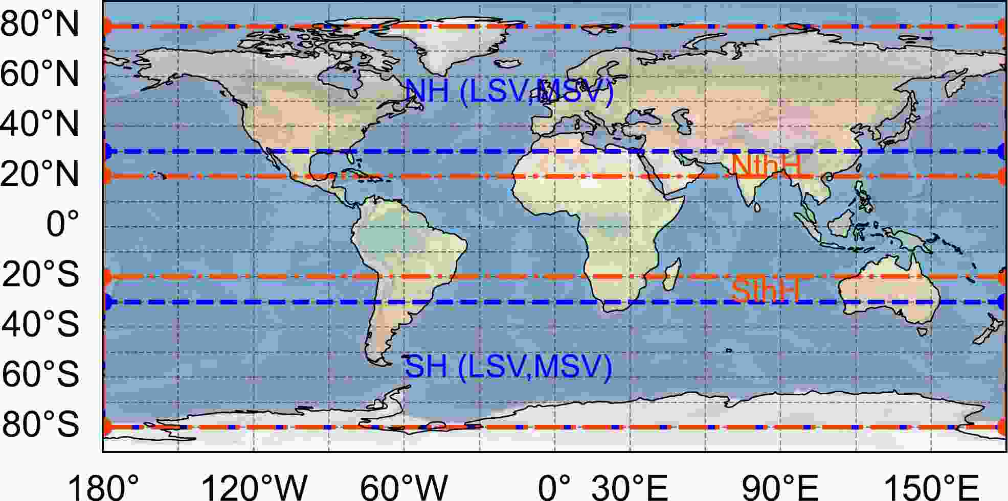
Figure 1. Forecast region of CMA-GEPS (Global). Shown are the target areas of LSV and MSV (NH and SH, blue dashed lines) and the verification regions for GEPS (NthH and SthH, orange dashed-dotted lines, details can be found in section 4.2).
However, mesoscale errors also influence the medium-range prediction skill, then the LSV is insufficient to detect mesoscale uncertainties. An MSV is set to capture meso-α- to synoptic scale uncertainties in meteorological systems over the target areas. The differences between MSV and LSV’s settings include the horizontal resolution (e.g., 1.5°) and OTI (e.g., 24 h). Previous studies have proven that increasing horizontal resolution leads to a reduction in the ability of the OTI to obtain fast-growing SVs in a reasonable manner (Buizza, 1994b; Wang et al., 2020; Ono et al., 2021).
It should be noted that, unlike previous studies, Ye et al. (2020) and Ono et al. (2021) used SVs of differing scales for REPS with higher resolution, while this study uses multiscale SVs for GEPS with lower resolution, considering that the main goal of GEPS is to provide guidance information about medium-range prediction. Therefore, the specific calculation settings of multiscale SVs differ from previous studies and are evaluated based on several sensitivity experiments.
-
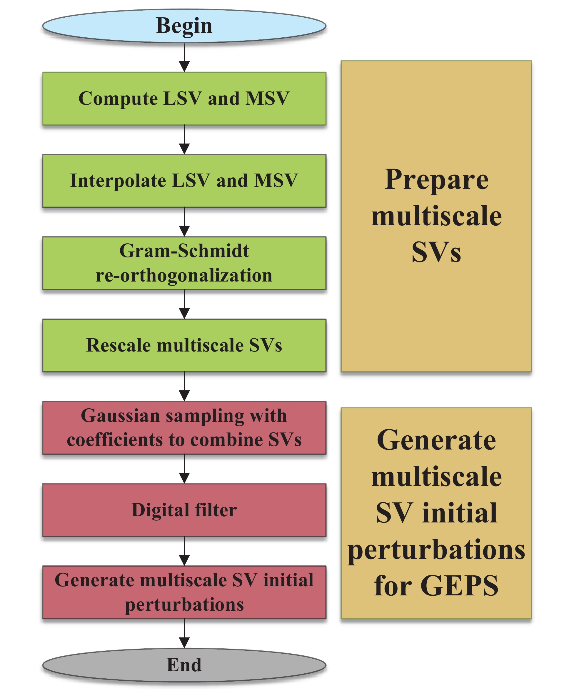
Since each type of SV can only reflect uncertainty information separately at distinguished meteorological scales, it is necessary to combine all multiscale SVs to generate initial perturbations that reflect uncertainties as much as possible with finite ensemble members. Meanwhile, the focus of this study is to determine a reasonable method for combining multiscale SVs to generate initial perturbations for the GEPS, according to the probability density function.
Before the combination procedure, the LSVs and MSVs are interpolated to the same horizontal resolution as the CMA-GEPS (e.g., 0.5°). Subsequently, using a Gram-Schmidt re–orthogonalization for each of the SVs ensures the removal of duplicate information. After that, it is necessary to adjust the amplitude of each type of multiscale SV according to the analysis error (
$ {e_u},{e_v},{e_\theta } $ and$ {e_\Pi } $ ) by a rescale operator$ {\bar L^2} $ defined as follows:where the overbar represents a mean over grid-point spaces, and N1 is the total grid points in the CMA-TLM. The analysis error is estimated from the CMA's four-dimensional variational data assimilation (CMA-4DVAR) system. Each perturbed variable has a reference analysis error that is related to target areas (NH and SH) and model level and varies according to the month in question.
Hence, the LSVs and MSVs, have a different
$ {\bar L^2} $ according to Eq. (7). Therefore, the matrix of the SVs in the real state (X), and their matrix in the Eulerian state ($ {\mathbf{\hat X}} $ ), can be described by:where γ is a constant factor to control the maximum acceptable ratio between perturbations amplitude and analysis error. After the rescaling procedure, the multiscale SV initial perturbations Pj are generated by:
where NNH and NSH denote the number of SVs in the NH and SH, respectively; αj,k denotes the random coefficients according to the Gaussian distribution, j and k denote the number of initial perturbations and SVs, respectively; coefficients β and δ determine the amplitude of the LSV’s and MSV’s perturbation at their initial states, respectively.
Finally, a digital filter method is used to modify abnormal values in the multiscale SV initial perturbations according to the triple reference analysis error which is estimated from the CMA-4DVAR.
The perturbed variables listed here include potential temperature and the u and v wind speeds. Subsequently, a pair of multiscale SV initial perturbations are added to or subtracted from the control forecast to generate ensemble members for CMA-GEPS. Each ensemble member has an equal probability. The experimental settings and parameters for the initial perturbations of multiscale SVs in this study are summarized in Table 2, and the main process of the multiscale SV approach is summarized in Fig. 2.
Experiment name Details of perturbation γ β δ LSV Only use LSV perturbation 0.05 0 0 MSV Only use MSV perturbation 0.045 0 0 MLSV1 Use multiscale SV perturbations 0.068 0.75 0.75 MLSV2 Use multiscale SV perturbations 0.068 0.5 0.5 MLSV3 Use multiscale SV perturbations 0.068 0.25 0.25 Table 2. Details of multiscale SV initial perturbation experiments.
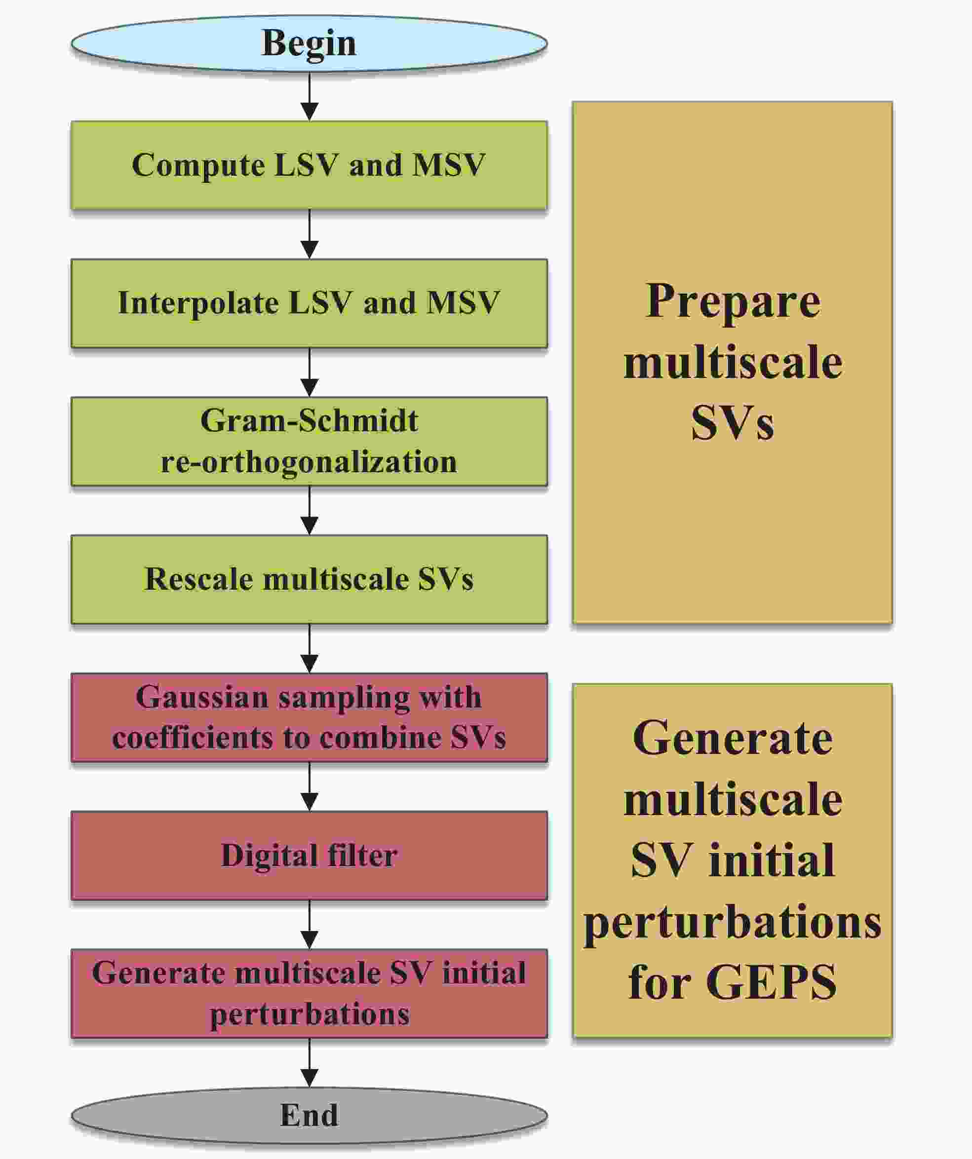
Figure 2. The main process of generating multiscale SV initial perturbations for GEPS.
Compared with the previous study, the JMA combines all SVs determined by the variance minimum rotation method for a regional EPS (Saito et al., 2011; Ono, 2020). The Gaussian sampling with coefficients method is introduced in this study, which combines all multiscale SVs to generate initial perturbations for GEPS with finite ensemble members. The purpose of coefficient settings is to explore whether the multiscale SV initial perturbations with different amplitudes can influence the prediction skills of the GEPS.
-
This study used the CMA-GEPS to carry out global ensemble forecast experiments. The CMA-GEPS was developed independently by the CMA’s Center for Earth System Modeling and Prediction, based on the CMA Global Forecast System (CMA-GFS) and has been running operationally since 2018 (Li et al., 2019; Shen et al., 2020; Peng et al., 2022). The control member (CTL, unperturbed member) of CMA-GEPS is initialized by CMA-4DVAR (the four-dimensional variational data assimilation system of the CMA) (Zhang et al., 2019), including 720 × 360 horizontal grid points with a resolution of 0.5° and 60 vertical layers. Furthermore, the five experiments of initial perturbation are added to and subtracted from the CTL to initialize the ensemble member in CMA-GEPS.
The multiscale SV characteristics and their performance in CMA-GEPS are analyzed based on a total of 32 cases for each experiment. To reduce the impact of test cases, representative months were selected from different seasons (JAN, APR, JUL, and OCT) for experimentation and verification. For each experiment, the same set of 10-day ensemble forecasts is initialized every fourth day (day 1, 5, 9, 13, 17, 21, 25, 29) for four months (total of 32 cases) at 0000 UTC. Heavy rainfall (≥25 mm (24 h)–1) cases mainly occurred in APR, JUL, and OCT, with 23 cases in total. The ensemble forecast time is 240 h and the forecast interval is 24 h. The configurations of CMA-GEPS in this study are summarized in Table 3.
Parameter CMA–GEPS Forecast region Global Resolution 0.5°, L60 Model top 3 hPa Forecast length 240 h Output frequency 24 h Initial condition CMA–4DVAR (upscaling) Initial perturbation method Single–scale SV or multiscale SV
(mentioned in section 2.2)Ensemble members 1 unperturbed member + 20 perturbed members Model perturbation method − Table 3. Configurations of CMA-GEPS for ensemble experiments
-
The structures and characteristics of SVs on multiscale are evaluated based on all 32 cases.
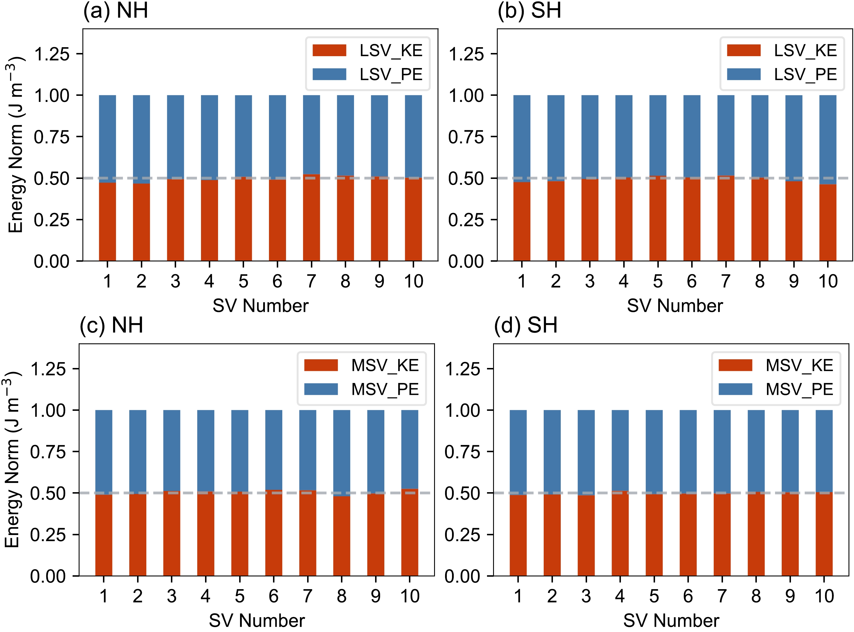
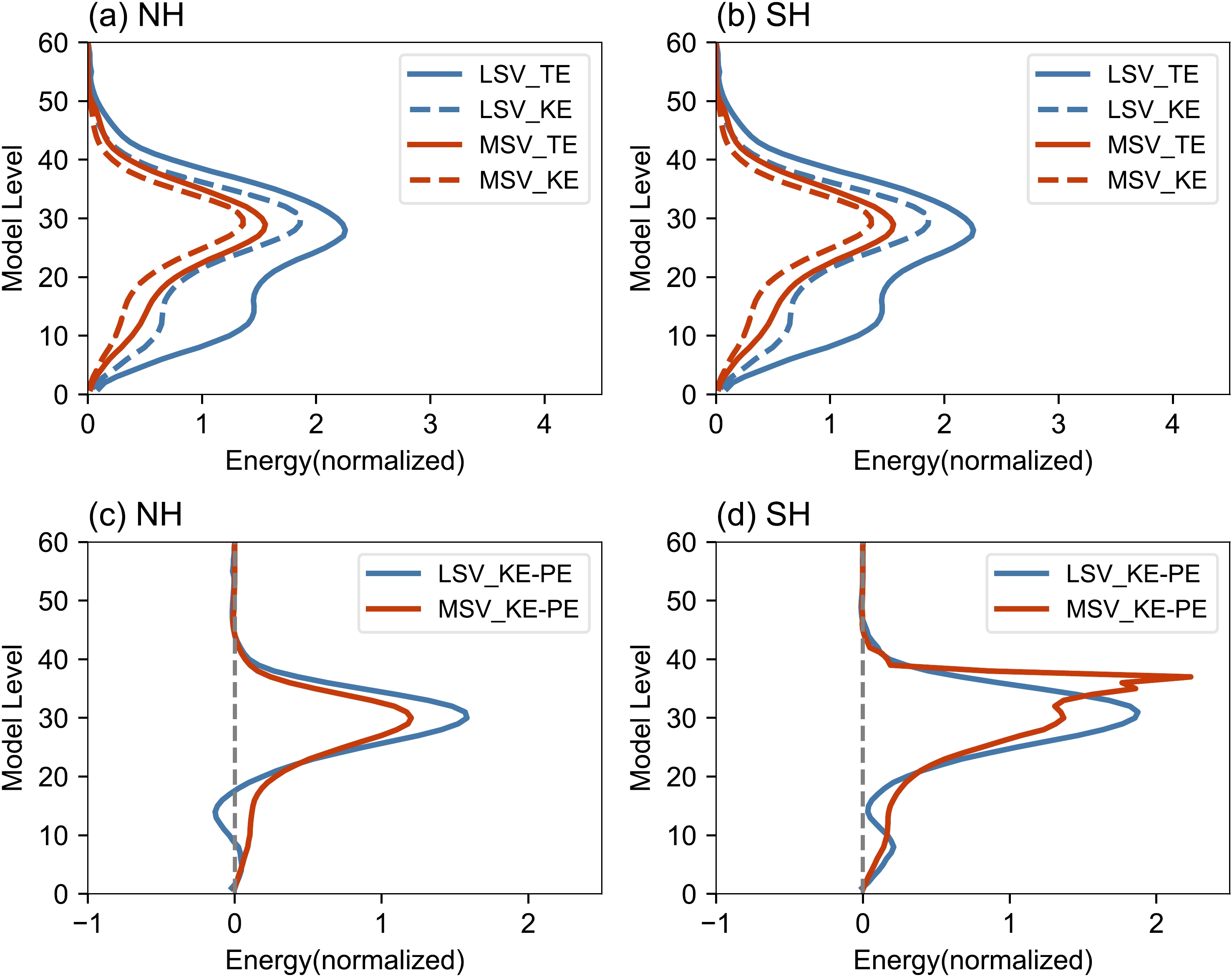
The energy partitioning of the first 10 multiscale SVs in terms of the kinetic energy (KE) and potential energy (PE) of the TE at the initial time was averaged in all cases and depicted in Fig. 3. The panels show that the ratio of KE to PE of the LSVs (Figs. 3a, b) and MSVs (Figs. 3c, d) is approximately 1:1 at the initial time over the NH and SH.
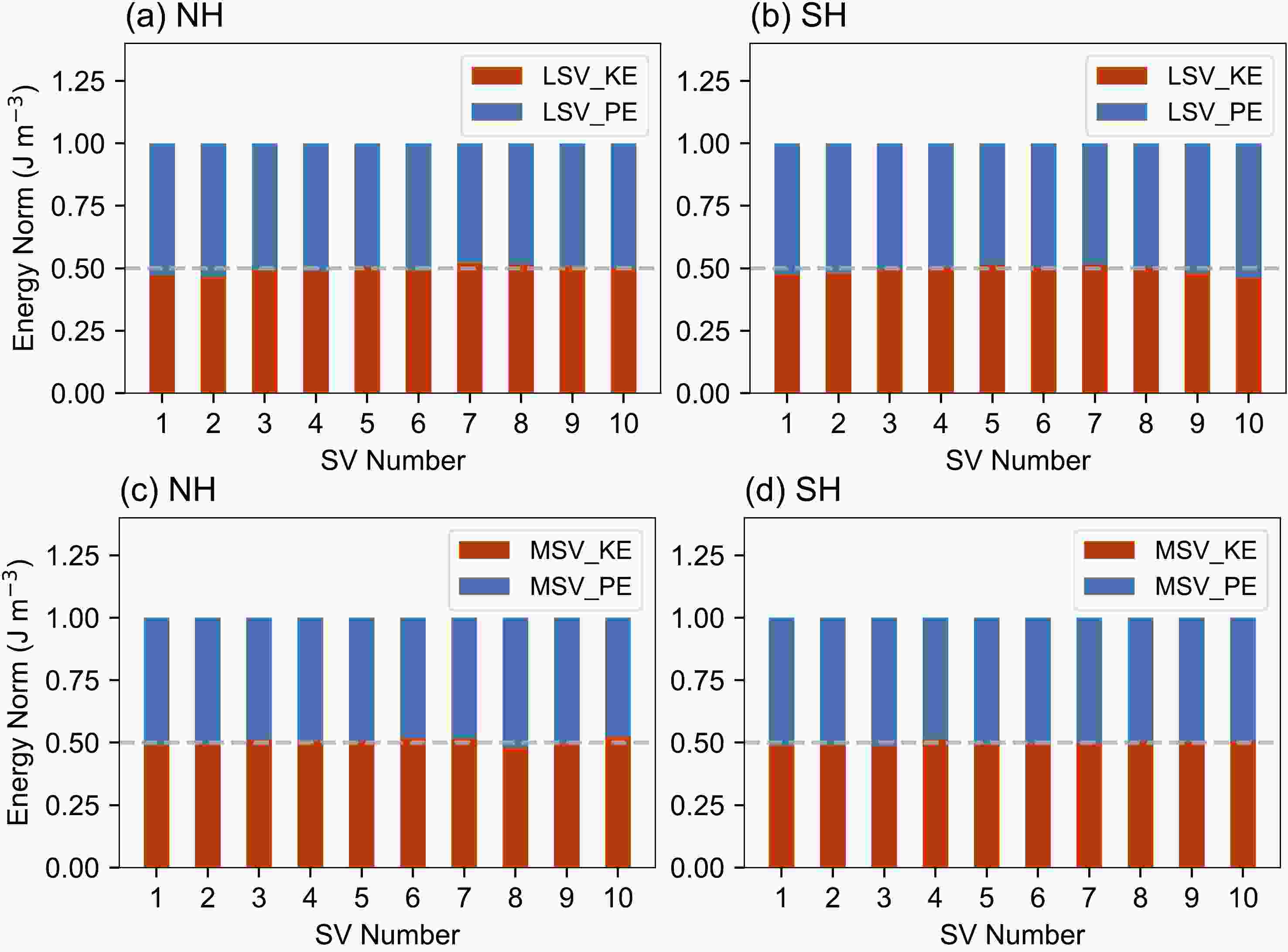
Figure 3. Energy partitioning of multiscale SVs in terms of their kinetic energy (KE, red) and potential energy (PE, blue) of the total energy at the initial time averaged over the (a, c) NH and (b, d) SH. The average is calculated from all the cases. The reference line (grey) is 0.5. Panels (a, b) indicate LSVs and (c, d) MSVs.
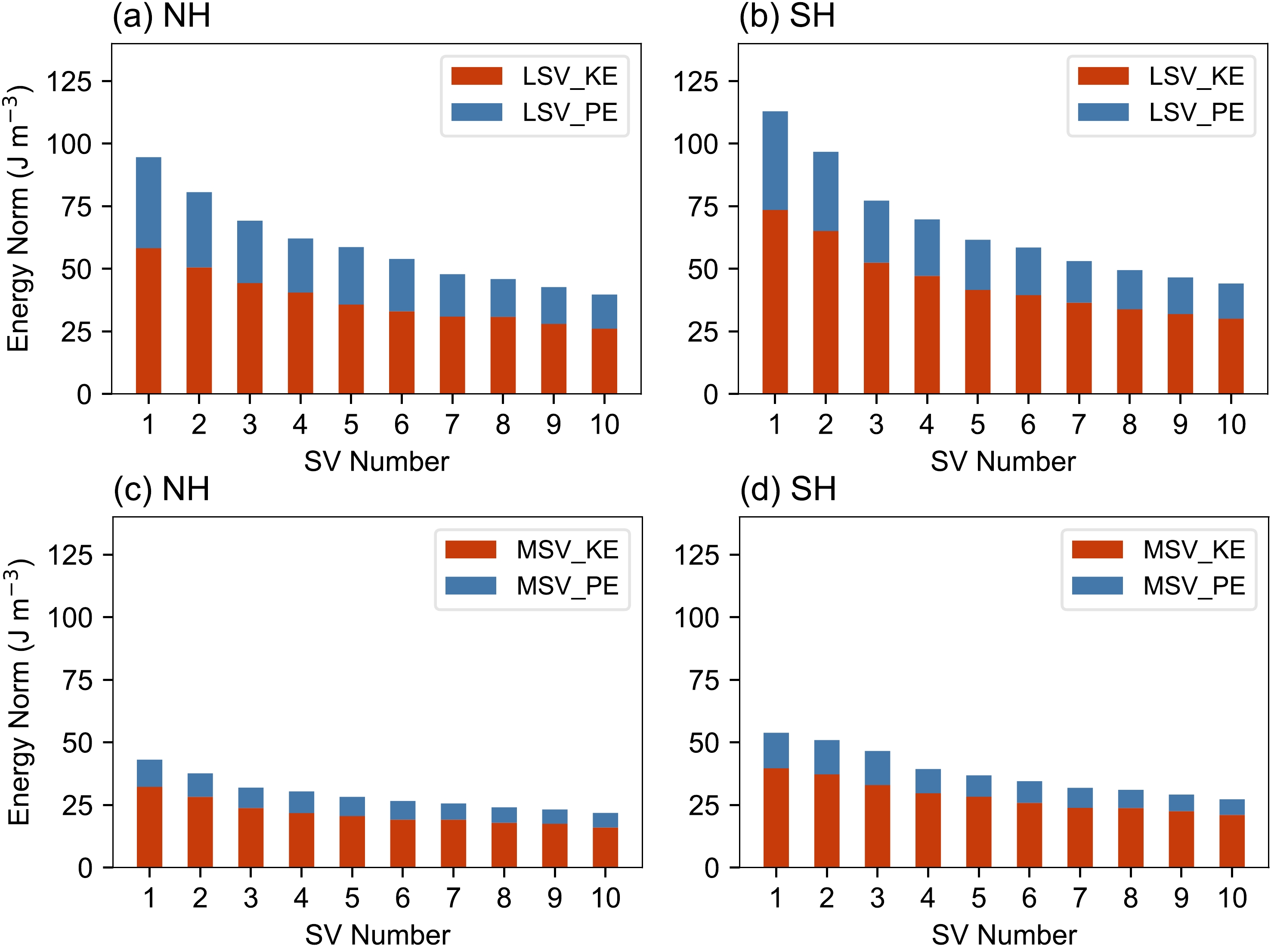
Figure 4 shows that the energy norm partitioning of multiscale SVs evolves over the OTI in TLM, respectively. The panels show that the ratio of KE to PE is almost 3:1 at the evolved time. Compared to the initial time, KE plays a dominant role at the evolved time. Usually, the dry-TE norm extratropical SVs are characterized by a dominant KE component at the evolved time. The transformation from an initial state dominated by PE to a final mainly KE state is associated with the adjustment processes. This is because dry-TE extratropical SVs evolve towards the leading Lyapunov vector, representing the maximum sustainable growth direction in a system without external forcing. Also, SV perturbations as physical structures have to satisfy particular dynamical properties, such as the linear balance equation in the TLM. Therefore, this transformation can be interpreted as the result of adjustment processes, causing the rotation of off-attractor SVs from initial time towards on-attractor SVs at evolved time.
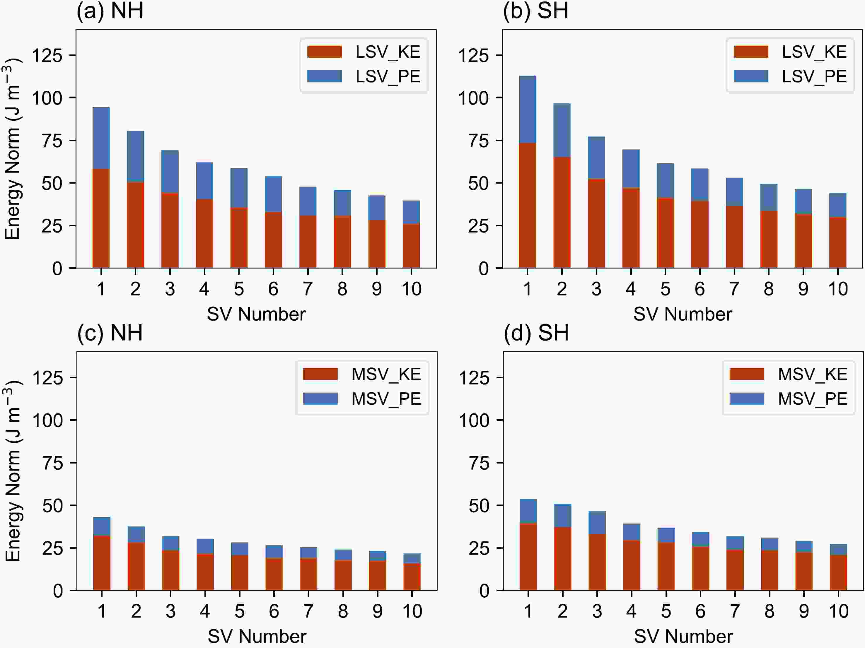
Figure 4. Same as in Fig. 3 but at the evolved time.
The vertical profile of the energy norm and the differences between KE and PE at the initial time of the SVs on multiscale averaged over the NH and SH are shown in Fig. 5. As shown in Figs. 5a and 5b, the energy maximum of the LSVs and MSVs is located in the lower to middle troposphere (layers 20–27, around 3000–5500 m above sea level) in the NH and SH. Meanwhile, it can be seen from Figs. 5c and 5d that the PE of the LSVs, and MSVs is dominantly located in the middle troposphere, while the KE is mostly in the upper troposphere (layers 31–33, around 9000 m above sea level).
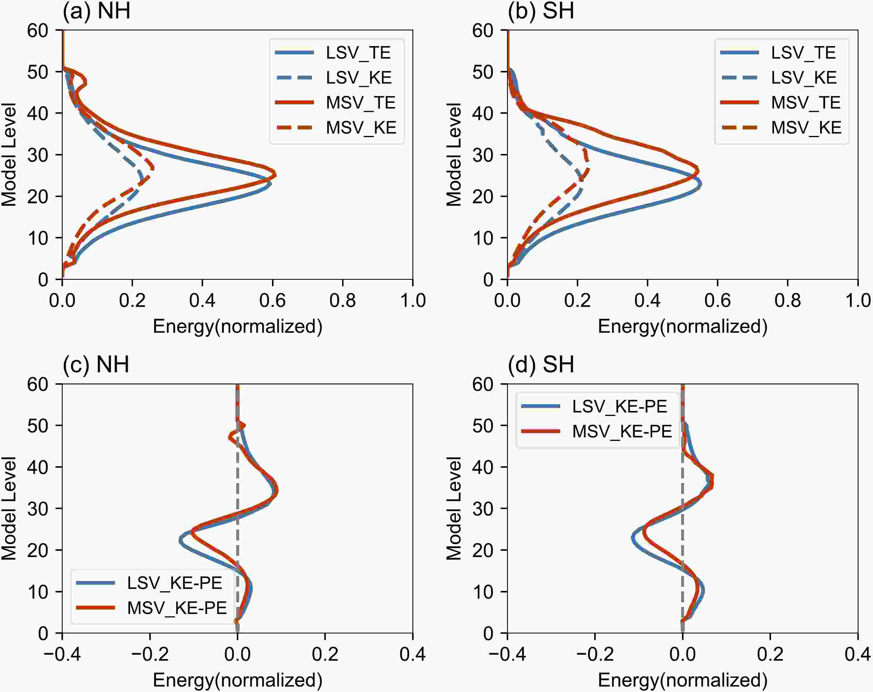
Figure 5. Vertical profiles of the (a, b) energy norm (TE, solid line; KE, dashed line) and (c, d) differences between KE and PE at the initial time of SVs on the multiscale. The average is calculated from all cases. The blue line is for the LSVs; the red line is for the MSVs.
The vertical profile of the energy norm and the differences between KE and PE at the evolved time of the SVs on multiscale averaged over the NH and SH are shown in Fig. 6, Which illustrates that both the LSV and MSV are dominated by KE in the troposphere at evolved time. It can be concluded that the PE located in the lower to middle troposphere is transformed into KE in the upper and lower layers. Additionally, it is possible to interpret the energy growth as the result of wave pseudomomentum propagating into the jet. These results are consistent with previous research (Buizza and Palmer, 1995; Ono, 2020; Ye et al., 2020; Wang et al., 2020, 2023).
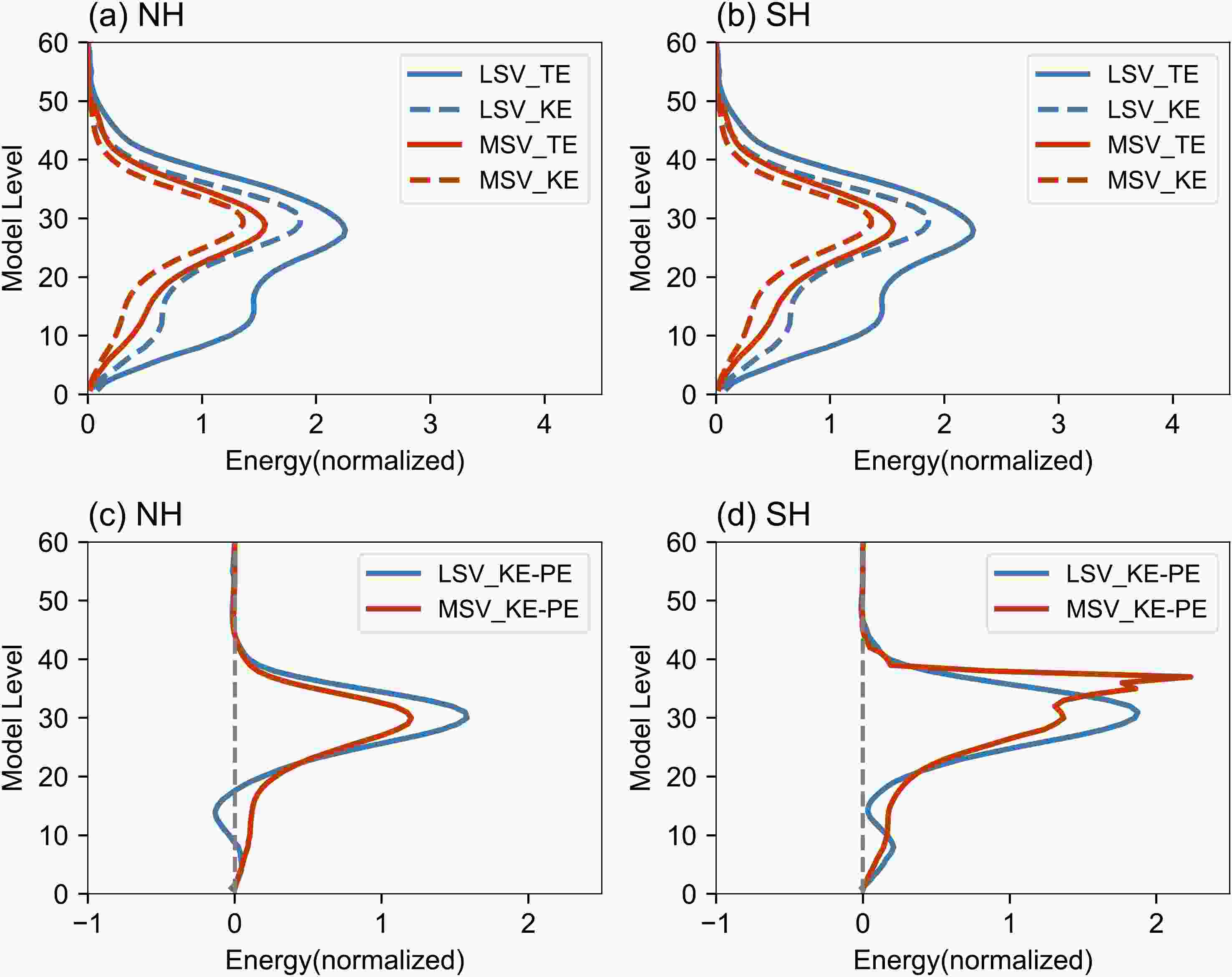
Figure 6. Same as in Fig. 5 but at the evolved time.
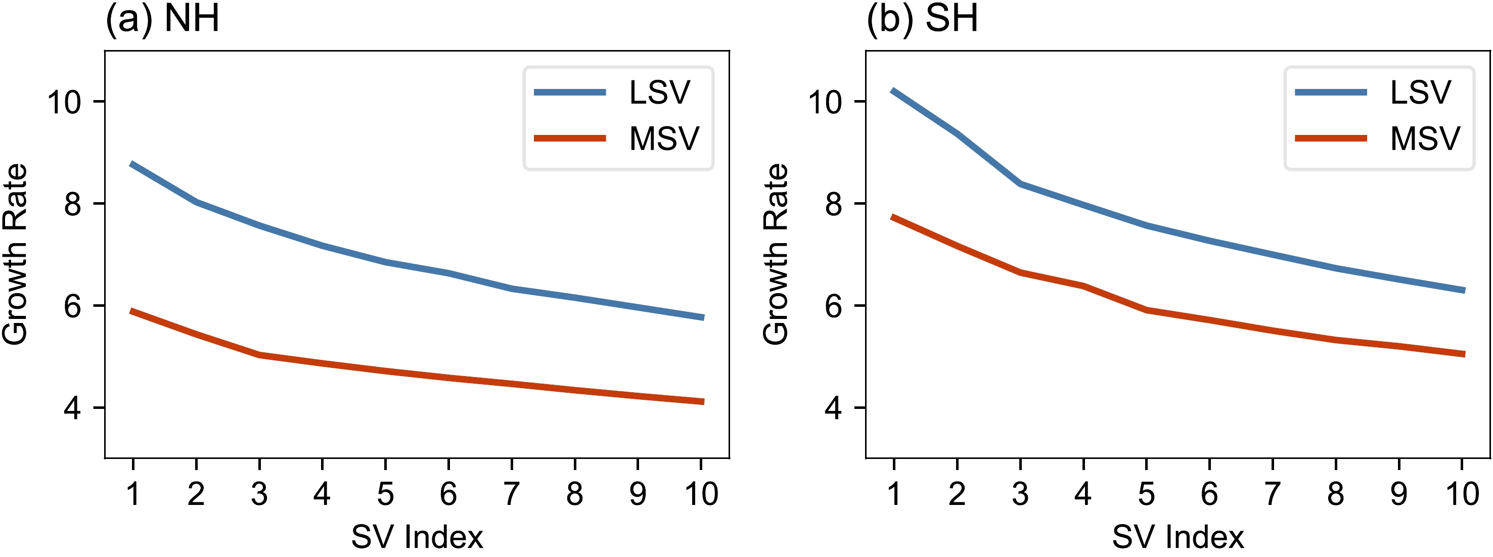
The growth rate of SVs is associated with singular values. Figure 7 shows the average growth rate of 10 leading multiscale SVs over the NH and SH (Figs. 7a and b, respectively). As shown in Figs. 7a and b, the growth rate of the LSVs is larger than those of the MSVs in the NH, which means that the LSVs contain more unstable uncertainty information. In terms of the growth rate of SVs in the SH, the LSV values are larger than those of the MSVs. In conclusion, the growth rate of the LSVs is > 5.0, while they are above 4 for MSVs. Thus, using finite multiscale SVs to generate initial perturbations can capture the fastest-growing uncertainty information about the atmosphere at the initial time.
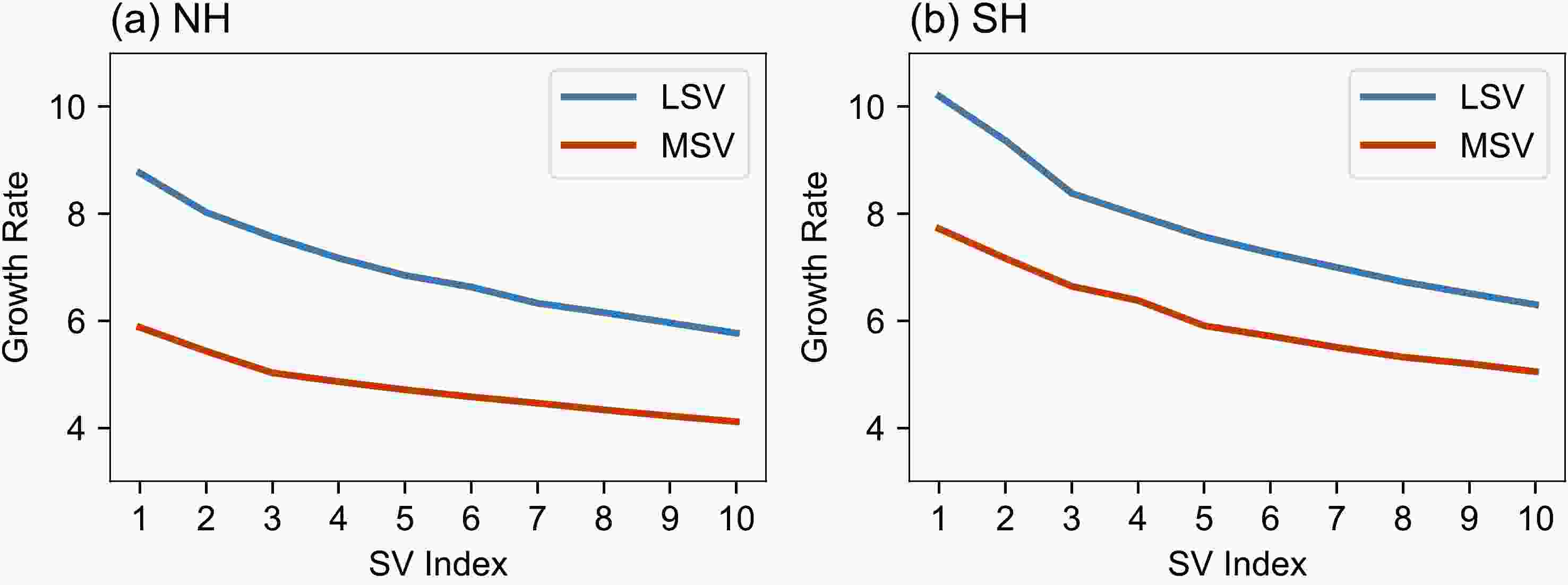
Figure 7. Growth rate of the 10 leading multiscale SVs over the (a) NH and (b) SH. The blue line is for the LSVs; the red line is for the MSVs. The average is calculated from all cases.
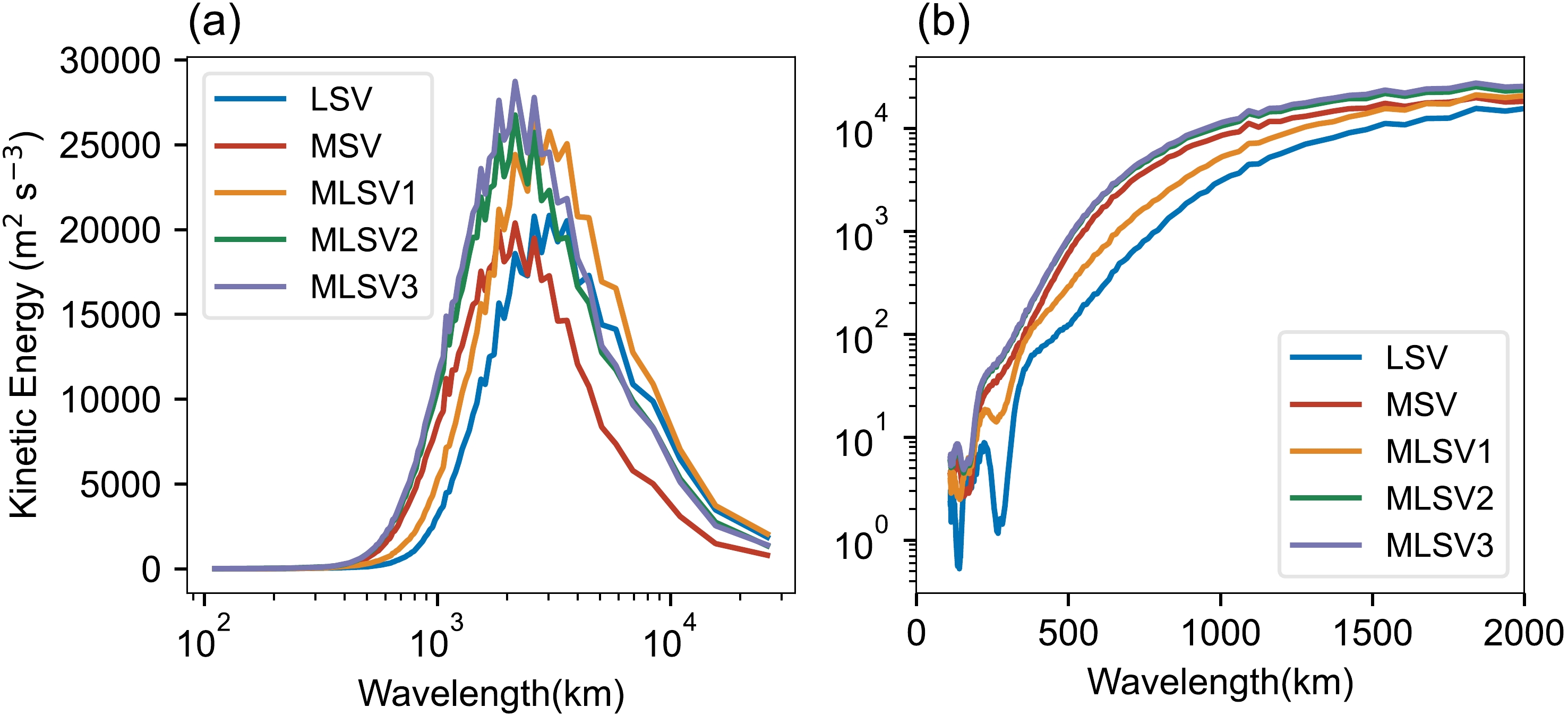
The kinetic energy spectrum is usually used to analyze the spatial scale characteristics of the initial perturbation. Figure 8 gives the averaged perturbation kinetic energy spectrum distribution for single-scale SVs and multiscale SVs in all cases. As can be seen from Figs. 8a and b, the 500-hPa kinetic energy spectrum of MSV is larger than that of the LSV at the mesoscale, and lower than that of the LSV at the synoptic scale. For multiscale SVs, the distribution of the kinetic energy spectrum is related to the proportion and amplitude of the initial perturbations of the multiscale SVs. For MLSV1 (LSVs dominate), it blends mesoscale to synoptic scale SVs so that it contains more perturbation kinetic energy at the multiscale than single-scale SV, especially at the synoptic scale. Due to the equal proportions of LSVs and MSVs, the kinetic energy of MLSV2 is larger than those of the LSV and MLSV1 at the mesoscale, and the MSV at the synoptic scale. For MLSV3 (MSVs dominate), the distribution of the kinetic energy spectrum is mostly the same as it is for the MSVs. However, MLSV3 contains more energy in the mesoscale than MSV. In conclusion, the initial perturbations of the multiscale SVs contain more energy than the single-scale SVs at different meteorological scales.
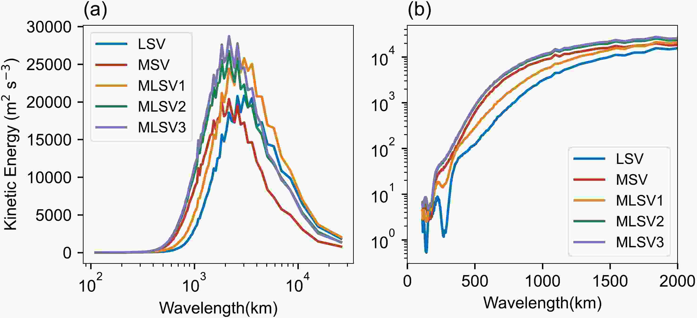
Figure 8. The 500-hPa kinetic energy spectrum distribution (a) for single-scale SVs (LSVs, blue line; MSVs, red line) and multiscale SVs (MLSV1, yellow line; MLSV2, green line; MLSV3, purple line) initial perturbations. The result of Fig. 8b is the same as in Fig. 8a but with a focus on the mesoscale. The average is calculated from all cases.
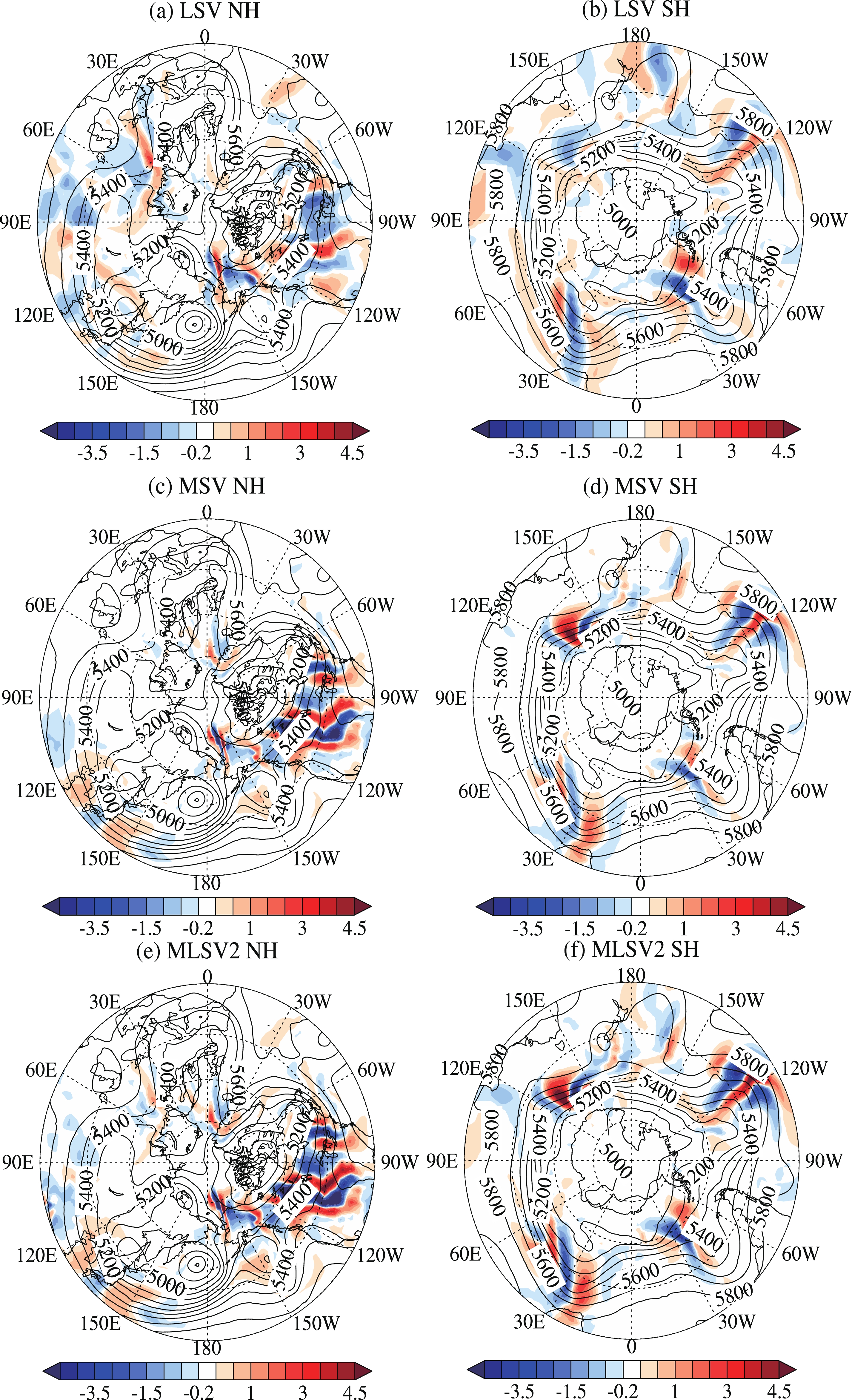
Figure 9 presents the horizontal structures of the initial perturbations in the NH and SH at the layer 26 model level (near 500 hPa) of the potential temperature. The primary distinctions between LSV and MSV initial perturbations include their distribution and amplitude. The LSV and MSV initial perturbations are in North America, central Europe, and East Asia characterized by trough or ridge regions. In contrast, the spatial distribution of the LSV initial perturbations is broader than that of the MSV. The MSV initial perturbations are more localized; meanwhile, the amplitude of their perturbations is larger than that of the LSV. In addition, the MSV initial perturbations can capture smaller-scale uncertainties than the LSV. However, the horizontal structure of the initial perturbations for MLSV2 contains most of the characteristics of the LSV and MSV. The initial perturbations of MLSV2 can reflect more multiscale uncertainty than single-scale SVs. In conclusion, multiscale SV initial perturbations are mainly located in the mid-to-high-latitudes of instability and can capture multiscale uncertainties in the target area.
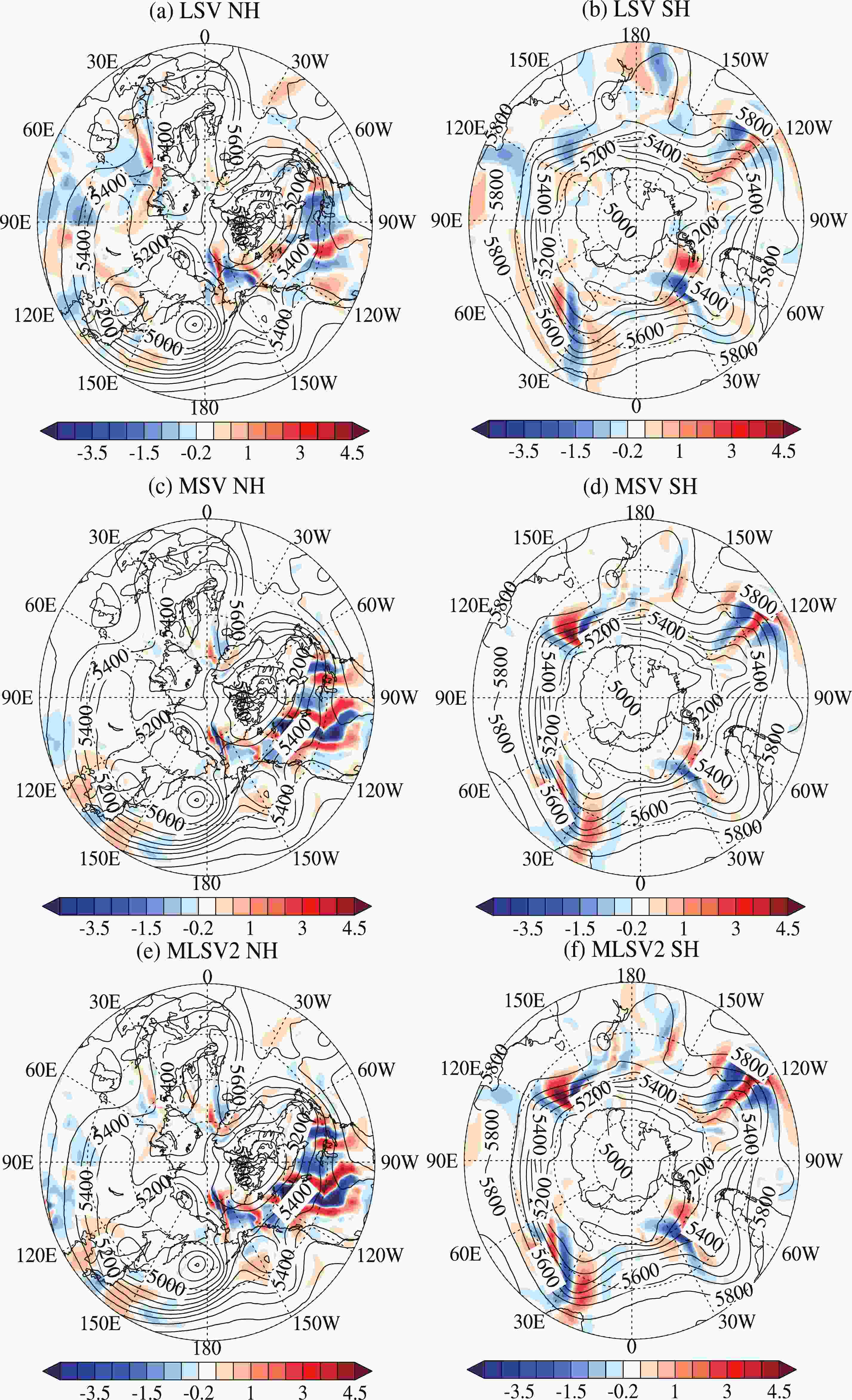
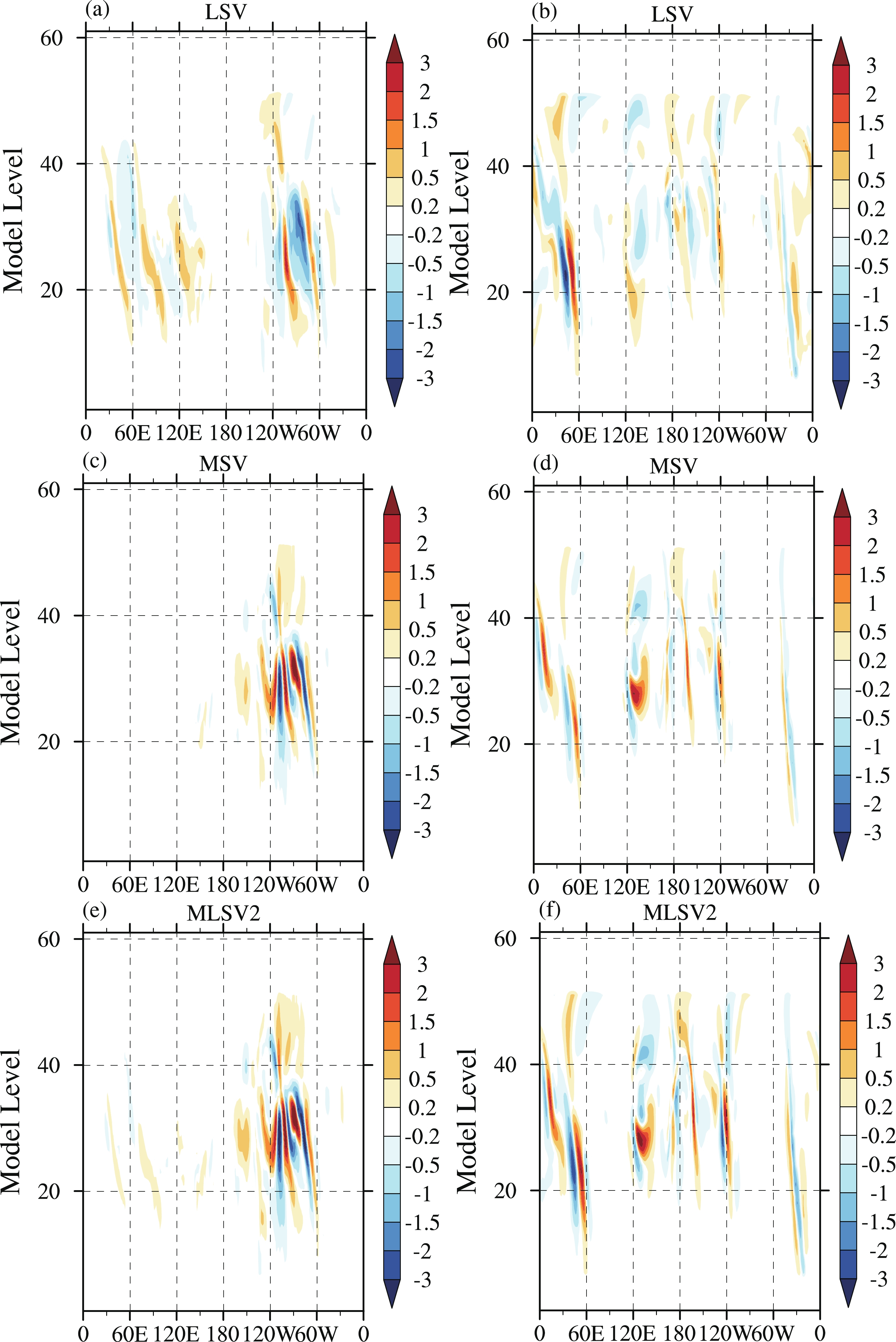
Figure 9. Horizontal distribution of initial perturbations (member 05) over the NH (first column) and SH (second column) at the layer 26 model level (up to around 5500 m) of the potential temperature (contours, unit: K) at the initial time (0000 UTC 1 January 2021). The black lines are the 500-hPa geopotential height of the CMA-4DVAR analysis. Panels (a, b) are generated from the LSV; (c, d) are generated from the MSV; (e, f) are generated from MLSV2.
Figure 10 shows the vertical cross-section structure of initial perturbations (member 05) at 50°N and 50°S of the potential temperature at 0000 UTC 1 January 2021. According to the vertical distributions of the initial perturbations in the LSV (Figs. 10a, b), MSV (Figs. 10c, d), and MLSV2 (Figs. 10e, f), a westward tilt with height exists at the initial time. Usually, such a vertical westward tilt is related to the baroclinically unstable atmosphere (Buizza and Palmer, 1995). Incidentally, an LSV can generate initial perturbations that are wider than those of MSVs, but MSV initial perturbations are generated with greater amplitude than LSVs. The MLSV2 initial perturbations retain most of the vertical structural characteristics of the LSV and MSV. Thus, MLSV2 initial perturbations contain the uncertainties of both the LSV and MSV at the multiscale.
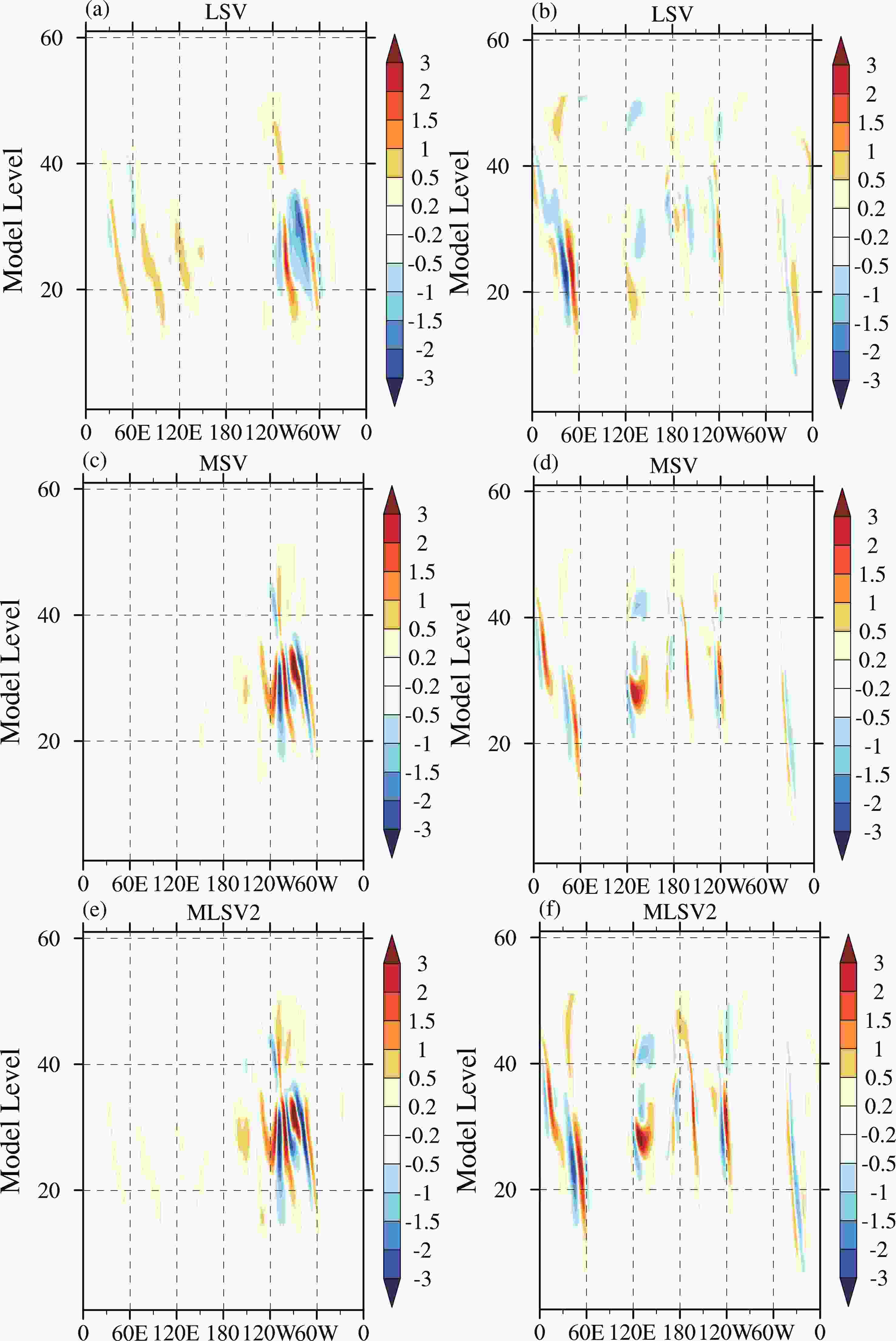
Figure 10. Vertical cross-section structure of initial perturbations (member 05) at 50°N (first column) and 50°S (second column) of the potential temperature (contours, units: K) (0000 UTC 1 January 2021). Panels (a, b) are generated from an LSV; (c, d) are generated from an MSV; (e, f) are generated from MLSV2.
In conclusion, multiscale SV initial perturbations retain the structure of single-scale SV initial perturbations. Both multiscale SVs have more PE than KE in the lower to middle troposphere at the initial time. During their growth, however, SVs are characterized by KE which is dominant in the upper and lower layers as the result of wave pseudomomentum propagating into the jet. Meanwhile, multiscale SV initial perturbations, are mainly located at the mid-to-high-latitudes and are associated with baroclinic instability. Meanwhile, multiscale SV initial perturbations can reflect the strongest dynamical instability in target areas. Furthermore, multiscale SV initial perturbations contain more perturbation kinetic energy in multiscale compared to single-scale SVs. Thus, multiscale SV initial perturbations have the ability to capture multiscale initial uncertainties with finite members.
-
In this study, the performances of multiscale SV initial perturbations on GEPS are evaluated by using a comprehensive set of forecast verification metrics, including the consistency, root-mean-square error (RMSE), ensemble spread, continuous ranked probability score (CRPS), anomaly correlation coefficient (ACC), and the area under the relative operating characteristic curve (AROC). Descriptions of these verification methods can be found in Stanski et al. (1989) and Buizza et al. (2005).
In this study, the main goal is to improve the ensemble forecast skill of a GEPS, as a GEPS plays an important role in operational NWP centers and provides probabilistic information about medium-range forecasts. Thus, the forecast verification metrics mentioned above of 850-hPa temperature, 500-hPa geopotential height, and 250-hPa u wind speed are computed. Internationally, operational NWP centers typically divide the Northern Hemisphere (NthH, 20°–80°N) and the Southern Hemisphere (SthH, 20°–80°S) for the verification of the GEPS (Buizza et al., 2005). Therefore, forecast verification metrics are weighted by the cosine of latitude prior to evaluation over the NthH and SthH. The CMA-4DVAR analysis is used as the true value for verification of forecast variables and China national meteorological stations data is used as the true value for precipitation verification. All of the forecast skill scores are calculated from all cases (total of 32) to compute the average, and a bootstrap algorithm (Hamill, 1999) is used to test the significance of the score differences between MLSV1 and the LSV.
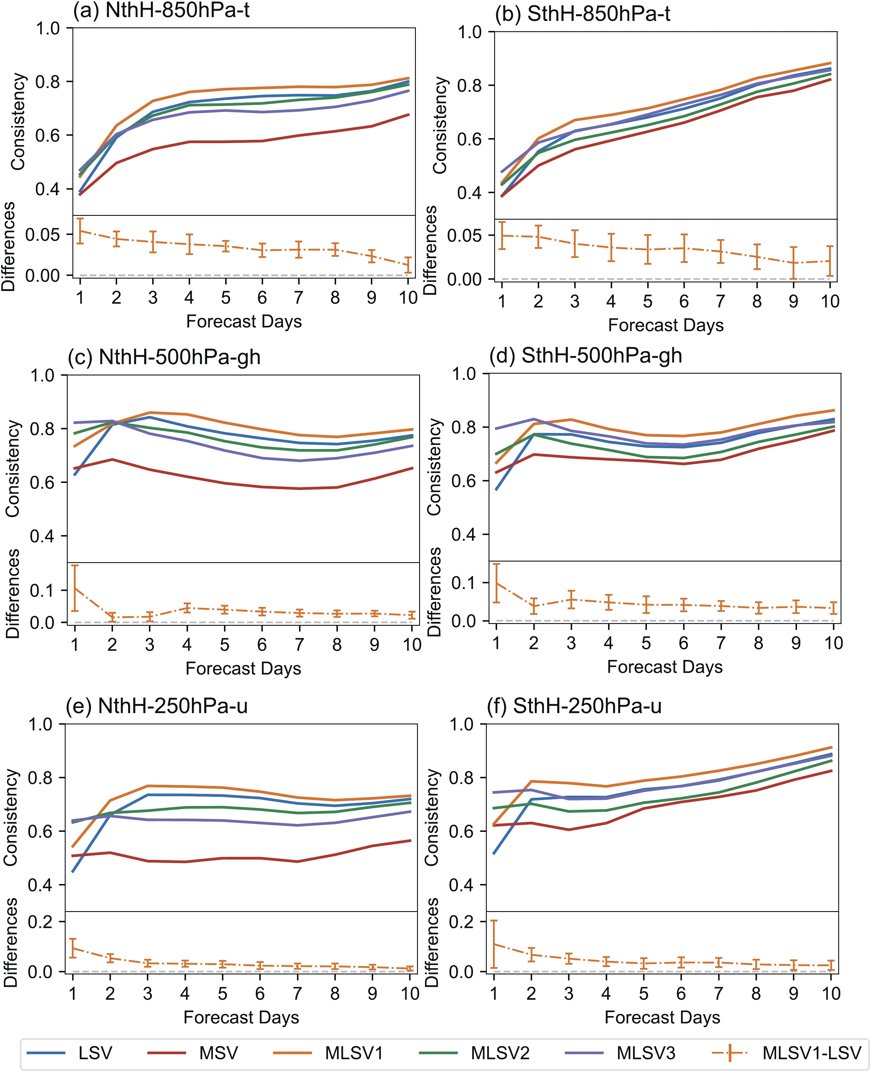
First, consistency is calculated as the ratio of the spread to the RMSE, and whether the ensemble spread is approximately equivalent to the RMSE becomes a metric to measure the reliability of an ensemble forecast system; the closer the consistency is to 1, the better the forecast. Figure 11 shows the time series of the consistency of different variables over the NthH and SthH. For single-scale SVs, the consistency of the LSV is better than that of the MSV, while for multiscale SVs, the consistency is related to the amplitude of multiscale SVs. Overall, multiscale SV experiments have performed better than single-scale SVs in GEPS. Specifically, the consistency of MLSV1 is significantly better than LSV and MSV. Furthermore, the performance of MLSV1 for medium-range global forecasting is the best among all experiments due to its higher proportion of LSV. In comparison, the consistency of MLSV3 is better than other experiments on short-range forecasting. Thus, the application of multiscale SV initial perturbations by a GEPS can significantly improve the consistency compared with single-scale SV initial perturbations in the context of short-to-medium-range global forecasting.
Figure 11. The time series of consistency scores of the ensemble mean LSV (blue line), MSV (red line), MLSV1 (yellow line), MLSV2 (green line), and MLSV3 (purple line). Values refer to the (a, b) 850-hPa temperature, (c, d) 500-hPa geopotential height, and (e, f) 250-hPa u wind speed over the (a, c, e) NthH (20°–80°N) and (b, d, f) SthH (20°–80°S). The consistency differences (MLSV1–LSV) are significant at the 95% confidence level when the values are outside the reference line (light-gray dashed line). The averages are calculated from all cases.
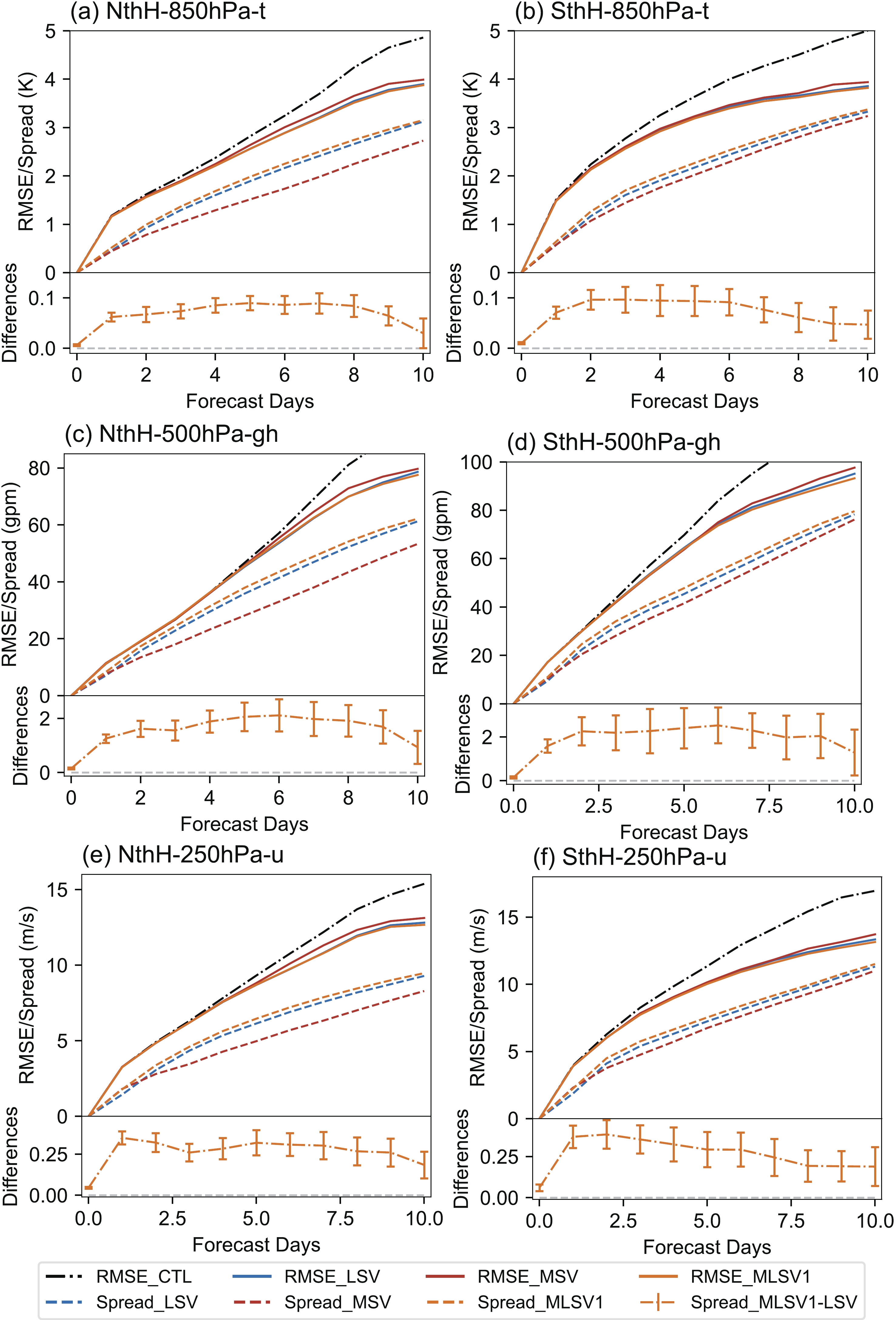
The consistency of the five ensemble forecast experiments has been analyzed above. It can be seen from Fig. 11 that the application of multiscale SV initial perturbations in CMA-GEPS can improve the ensemble forecast skill for different variables, so the analysis below focuses on the MLSV1 ensemble forecasts. However, the consistency only reflects the equilibrium relationship between the RMSE and the ensemble spread. To obtain a clearer understanding of the effect of multiscale SV initial perturbations on CMA-GEPS, the following analysis focuses on the details of the RMSE and its spread at all lead times. Figure 12 shows the averaged RMSE and spread for different variables over the NthH and SthH. Here, it can be seen that RMSEs increase steadily with forecast time and the RMSE of the ensemble mean forecasts from all experiments is lower than that of CTL during the medium-range forecast period. However, there are differences in the RMSE characteristics of multiscale SV ensemble experiments. For single-scale SV experiments, the performance of LSV is better than MSV due to the lower RMSEs during the latter half of the medium-range forecast period; for multiscale SV experiments, the RMSEs of MLSV1 are lower than all single-scale SV ensemble experiments from day 9 to day 10. The decrease in RMSEs during the last quarter of the medium-range forecast period indicates that adding multiscale SV initial perturbations is beneficial for GEPS.
Figure 12. Time series of RMSEs (solid line) and ensemble spread (dashed line) of the control experiments (CTL, black dashed-dotted line) and multiscale SVs experiments for the (a, b) 850-hPa temperature, (c, d) 500-hPa geopotential height, and (e, f) 250-hPa u wind speed for the LSV (blue line), MSV (red line) and MLSV1 (yellow line) experiments over the (a, c, e) NthH (20°–80°N) and (b, d, f) SthH (20°–80°S). The ensemble spread differences (MLSV1–LSV) are significant at the 95% confidence level when the values are outside the reference line (light-gray dashed line). The average is calculated from all cases.
The ensemble spread expresses the distance between the ensemble members and the ensemble mean to indicate the range and amplitude of the perturbation. Therefore, the spread should be large enough and should also maintain a reasonable proportionality with the RMSE to ensure the predictability of a GEPS. It can be seen from Fig. 12 that the ensemble spread from all experiments continues to increase with forecast time. For the single-scale SVs, the spread of the LSV is larger than that of the MSV during the medium-range forecast period. For multiscale SVs, the ensemble spread of MLSV1 is significantly larger than that of single-scale SVs during the short-to-medium-range forecast period. These results are consistent with the energy spectrum analysis mentioned earlier. When the kinetic energy of the initial perturbations is primarily located at the synoptic scale, they contain more uncertainties and unstable directions, leading to a continuous increase in the ensemble spread.
It can be seen from Figs. 11 and 12 that the application of multiscale SV ensemble experiments performs better than single-scale SVs at different isobaric surfaces, so the analysis below focuses on the 500-hPa geopotential height.
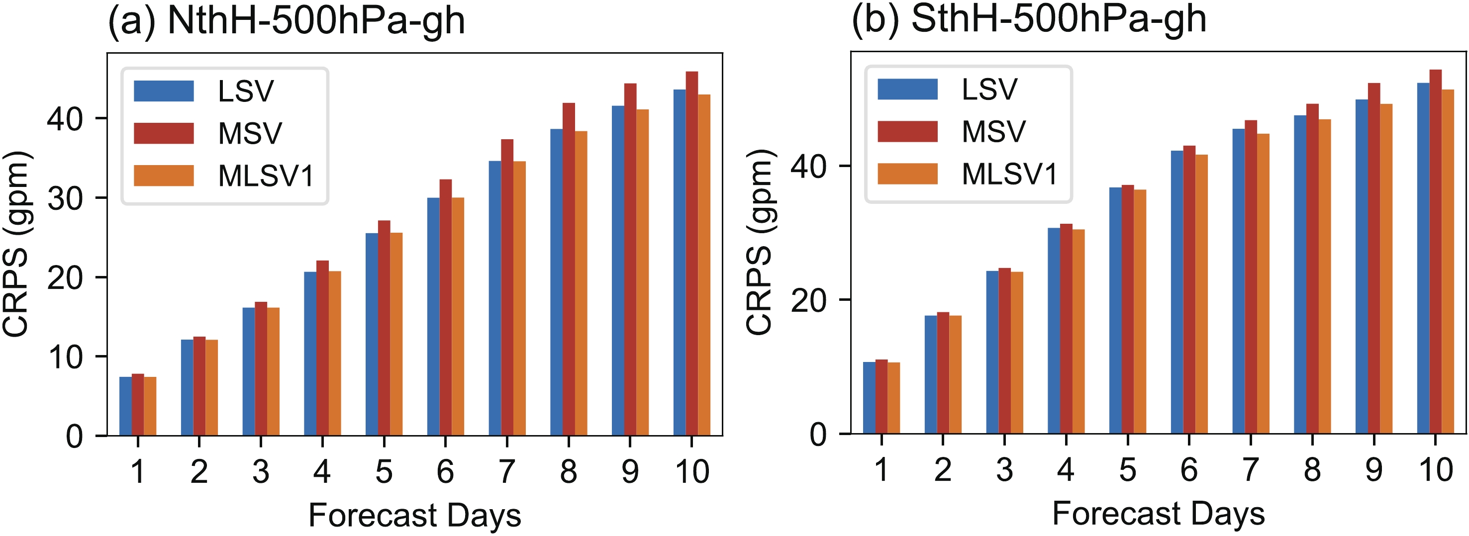
The CRPS is an important score for ensemble forecast verification and is calculated by the sum of the squared difference between the cumulative distribution function (CDF) of the forecasted probabilities and the CDF of the observations. The smaller the CRPS value, the smaller the difference between the predicted probability density and the observation, and the higher the prediction ability of the system. Figure 13 shows the averaged CRPS for the 500-hPa geopotential height over the NthH and SthH. It can be concluded that the CRPSs of LSVs are lower than MSVs during the forecast time. In addition, the CRPSs of MLSV1 are lower than single-scale SVs during the late forecast period in the NthH. Moreover, during the medium-range forecast period in the SthH, the CRPS of MLSV1 is also lower than that of single-scale SVs. Therefore, the application of multiscale SV initial perturbations in GEPS can improve the skill of probability forecasts, particularly during the late forecast period, especially in the SthH.
Figure 13. Time series of CRPS scores of the LSV (blue), MSV (red), and MLSV1 (yellow) experiments for the 500-hPa geopotential height over the (a) NthH (20°–80°N) and (b) SthH (20°–80°S). The average is calculated from all cases.
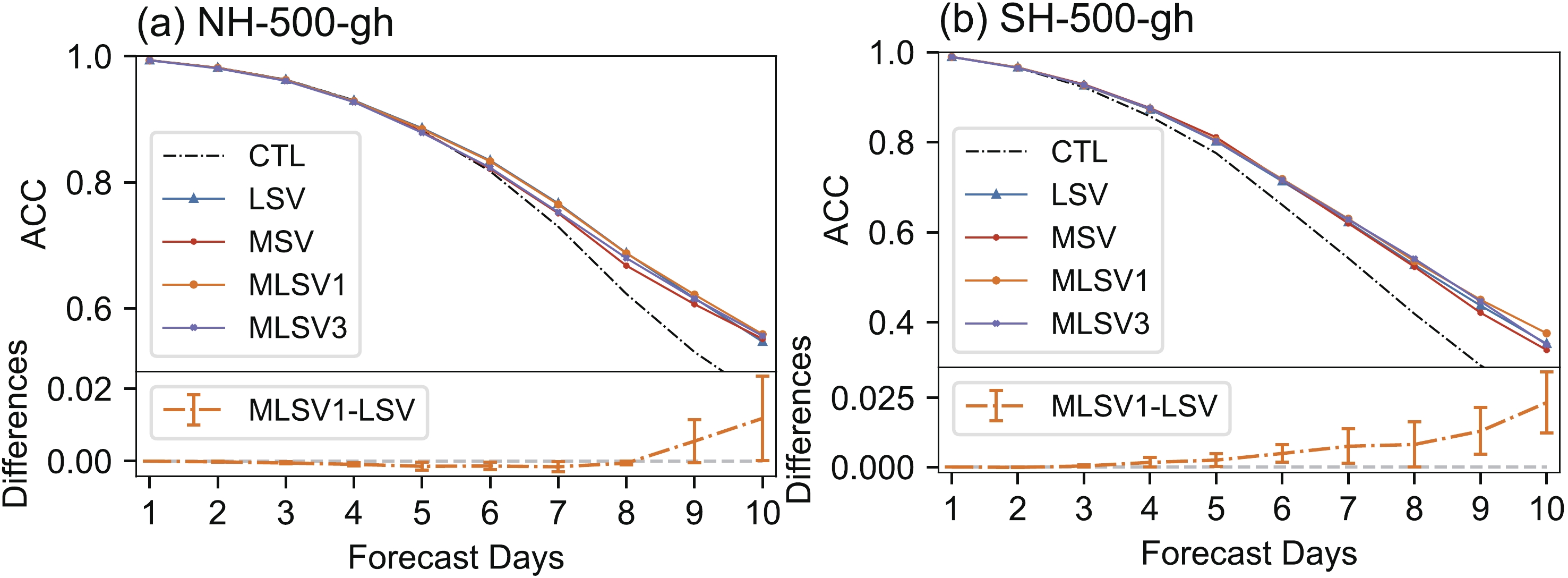
To further analyze the prediction skill of the GEPS, Fig. 14 presents the ACC of the 500-hPa geopotential height over the NthH and SthH. When the ACC is closer to 1, it implies a higher level of prediction skill. It can be seen from Fig. 14 that the results of the ensemble experiments are better than that of the CTL, but there are differences in the details summarized as follows. For single-scale SVs, the ACCs of the LSV are better than that of the MSV, which indicates that the forecast skill of the LSVs is better than that of the MSVs. For multiscale SVs, the ACCs of MLSV1 are similar to the LSV during the forecast time, but the ACCs of MLSV1 are larger than those of the LSV during days 9 and 10 over the NthH. In addition, the ACCs of MLSV1 are significantly larger than those of the LSV during the last half of the medium-range forecast period over the SthH. However, the ACCs of MLSV3 are lower than that of MLSV1 and LSV during the forecast period. These findings suggest that the use of multiscale SV initial perturbations with varying amplitudes can influence the prediction skills of GEPS. In conclusion, the application of multiscale SV initial perturbations improves the ensemble prediction skill of the medium-range atmospheric circulation in the SthH compared to a single-scale SV.
Figure 14. Time series of ACC scores of the LSV (blue), MSV (red), MLSV1 (yellow), and MLSV3 (purple) experiments for the 500-hPa geopotential height over the (a) NthH (20°–80°N) and the (b) SthH (20°–80°S). The ACC differences (MLSV1–LSV) are significant at the 95% confidence level when the values are outside the reference line (light-gray dashed line). The ensemble mean of all cases is used to calculate their average.
The reasons for these differences in verification might be related to the scales of perturbations and weather systems. For example, meso-α scale to synoptic scale errors usually have a more significant impact on the medium-range forecast predictability, as the meso-α scale to synoptic scale errors tend to act for a relatively long period. While meso-γ- to meso-β-scale weather systems are only active for a relatively short period, as such they tend to have localized characteristics and impact the short-range forecast. Meanwhile, the scale of LSV initial perturbations is proven to be larger than those of an MSV (section 4.1). Therefore, the medium-range forecast performance of an LSV is better than an MSV. However, it can be concluded that multiscale SV initial perturbations remain the main characteristics of single-scale SVs. Also, multiscale SV initial perturbations contain more kinetic energy than single-scale SVs, meaning that multiscale SV initial perturbations can capture the most unstable directions, which identify the fast-growing directions of the multiscale initial uncertainty that are responsible for the largest forecast uncertainty. Thus, the multiscale SV initial perturbation method can improve the performance of GEPS during the medium-range forecast period.
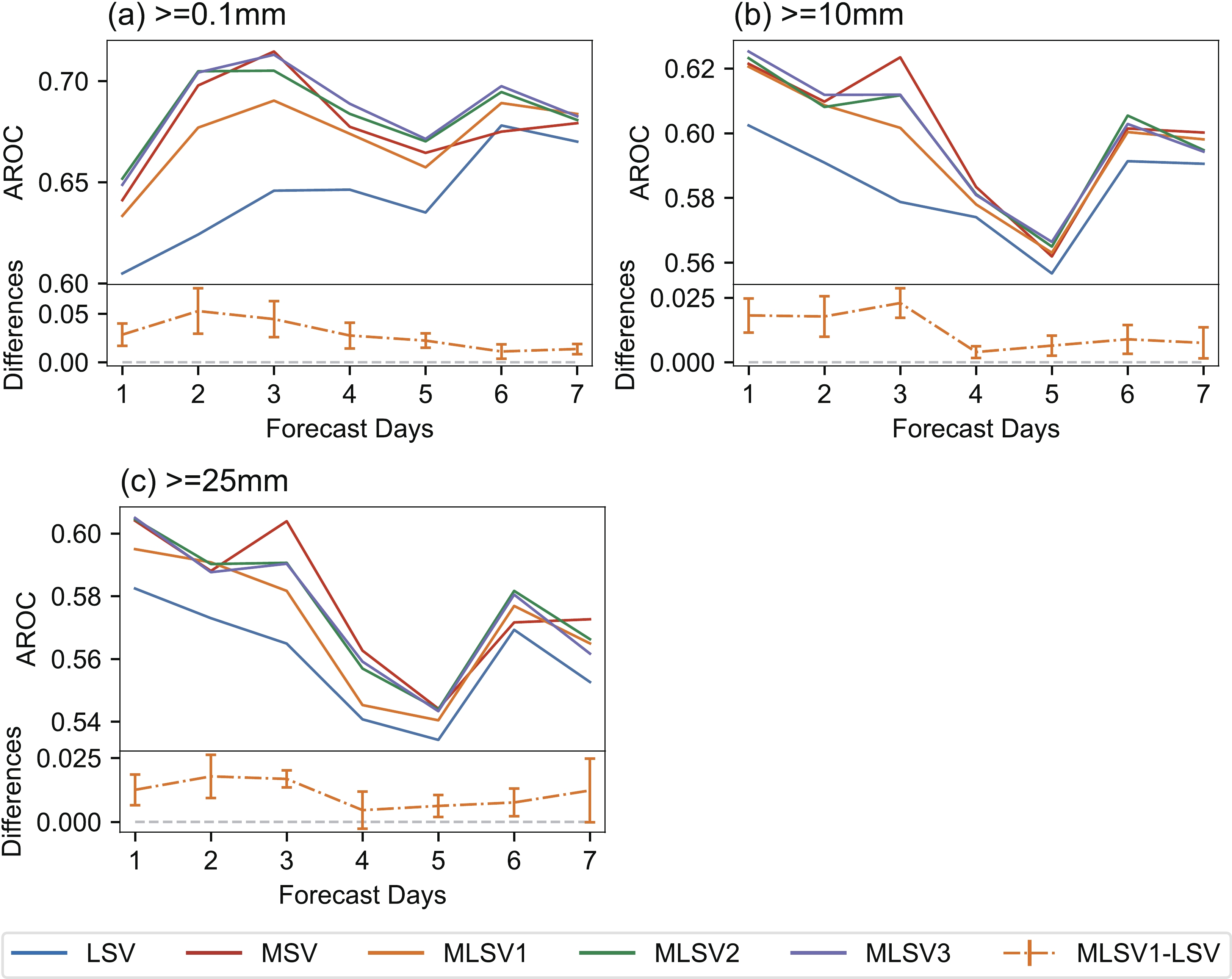
The AROC metric is commonly used to evaluate the performance of GEPS on precipitation. It is calculated by integrating the values of the ROC curve, which measures the ability of the forecast to discriminate between two alternative outcomes. The score of the AROC is greater than 0.5, noting that the closer this score is to 1, the better. Figure 15 presents the time series of the AROC for cumulative precipitation with a forecast time of 24 h in the Chinese region for light rain, moderate rain, and heavy rain (Figs. 15a–c). The results show that the AROCs of all experiments are greater than 0.5 during the forecast time. For the single-scale SVs, the AROCs of an MSV are better than that of an LSV at different precipitation levels. For the multiscale SVs, the AROCs of MLSV2 and MLSV3 are similar to that of the MSV, while that of MLSV1 are similar to LSV. Nevertheless, the AROCs of all multiscale SV ensemble experiments are greater than those of the LSV. In addition, MLSV2 and MLSV3 perform better than MSV during the last half of the forecast period for light rain and have greater scores from day 5 to day 7 for moderate and heavy rain. It can be deduced that MSV initial perturbations capture more uncertainties at the mesoscale, which are closely related to rainfall systems. Thus, the performance of the precipitation forecast using an MSV is better than the other experiments in the short-range forecasts. However, multiscale SV initial perturbations are more beneficial for a GEPS than those of an MSV. Because the AROCs of multiscale SV ensemble forecasts are greater than those using an MSV during the medium-range forecast period, the multiscale SV initial perturbation method is also beneficial for the precipitation forecast.
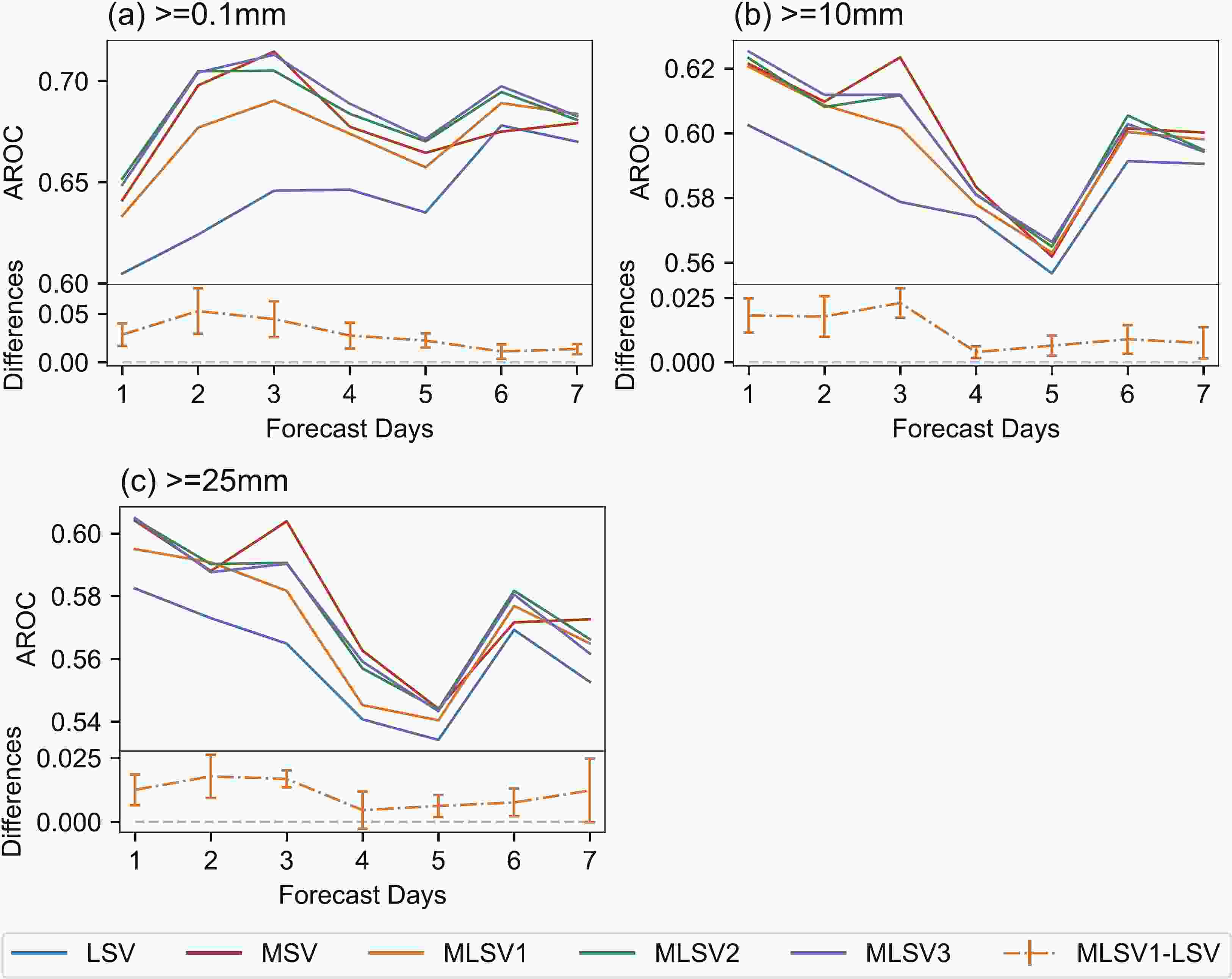
Figure 15. AROC scores for the precipitation greater than (a) 0.1 mm (light rain), (b) 10 mm (moderate rain), and (c) 25 mm (heavy rain) for the LSV (blue), MSV (red), MLSV1 (yellow), MLSV2 (green), and MLSV3 (purple) experiments. The AROC differences (MLSV1–LSV) are significant at the 95% confidence level when the values are outside the reference line (light-gray dashed line). The average is calculated from all experiments except for those with missing values (23 cases total).
-
A multiscale SV initial perturbation method for capturing the multiscale characteristics of ICs was developed based on the CMA global TLM and adjoint model, with the goal of detecting synoptic scale (LSV) and mesoscale (MSV) uncertainties for GEPS. In this study, the structures of multiscale SVs were analyzed from different perspectives, including the energy norm, energy spectrum, horizontal distribution, and vertical distribution, based on a total of 32 cases in different seasons. Finally, we also compared the performances of multiscale and single-scale SV initial perturbations in CMA-GEPS using the main metrics such as consistency, RMSE, spread, CRPS, ACC, and AROC.
At the initial time, the ratio of KE to PE of the LSVs and MSVs is approximately 1:1. Initially, the PE of multiscale SVs was located in the lower to middle troposphere; however, as time evolved, SVs became dominantly characterized by KE in the upper and lower layers as the result of wave pseudomomentum propagating into the jet. In addition, the growth rate of the LSVs is > 5.0, while they are above 4 for the MSVs. Thus, using finite multiscale SVs can capture the most fast-growing perturbations associated with multiscale uncertainty at the initial time.
The spectrum results and structures of multiscale SV initial perturbations show that multiscale SVs contain more energy than single-scale SVs at different meteorological scales. Specifically, the MLSV initial perturbations contain more perturbation kinetic energy at meso-to-synoptic scales and can capture more uncertainty information than single-scale SVs. Meanwhile, multiscale SV initial perturbations retain the characteristics of single-scale SVs in horizontal and vertical layers. Furthermore, multiscale SV initial perturbations present a westward tilt with height at the initial time and are mainly located in the mid-to-high latitudes which is associated with baroclinic instability. To summarize, multiscale SV initial perturbations can reflect the strongest dynamical instability and identify the directions of the initial uncertainty that are responsible for the largest forecast uncertainty with finite members.
Finally, the performances of multiscale SV initial perturbations in CMA-GEPS were verified. First, the GEPS that applied multiscale SV initial perturbations could significantly improve consistency compared to those that used single-scale SV initial perturbations on short-to-medium-range global forecasting. Second, the decrease in RMSEs during the last quarter of the medium-range forecast period indicates that adding multiscale SV initial perturbations is beneficial for the GEPS. Third, the ensemble spread of MLSV1 increases steadily and is significantly larger than that of single-scale SVs during the short-to-medium-range forecast period. Fourth, applying multiscale SV initial perturbations in the GEPS can improve the medium-range probability forecast more so than single-scale SVs. Fifth, multiscale SV initial perturbations can improve the atmospheric circulation ensemble prediction skill in the NthH and SthH compared with single-scale SVs. In the end, the multiscale SV initial perturbation method is also beneficial to precipitation forecasts during the forecast period. It can be concluded that capturing multiscale initial uncertainties and dynamically unstable information to generate initial perturbations is necessary and can improve the performance of a GEPS. However, the performance of a GEPS is sensitive to the amplitude of the multiscale initial perturbation amplitude. Overall, applying the multiscale SVs initial perturbation method can improve the forecast skill of CMA-GEPS.
Acknowledgements. We sincerely appreciate Kosuke ONO of JMA, Falko JUDT of NCAR, and Xiaoli LI of CEMC for giving us valuable information and helpful advice. Also, the comments of two anonymous reviewers helped to improve the quality of the manuscript. The research was supported by the Joint Funds of the Chinese National Natural Science Foundation (NSFC) (Grant No. U2242213), the National Key Research and Development (R&D) Program of the Ministry of Science and Technology of China (Grant No. 2021YFC3000902), and the National Science Foundation for Young Scholars (Grant No. 42205166).
| LSV | MSV | |
| Target area | 30°–80°N (NH) 30°–80°S (SH) |
30°–80°N 30°–80°S |
| Resolution | 2.5° | 1.5° |
| OTI | 48 h | 24 h |
| Norm | Dry TE | Dry TE |
| linearized physical processes (dry) |
Subgrid–scale orographic effect, vertical diffusion |
Subgrid–scale orographic effect, vertical diffusion |
| No. of SVs | 10 | 10 |


 AAS Website
 AAS WeChat