


 DownLoad:


-
Large-scale circulations, mesoscale currents, submesoscale currents, small-scale boundary-layer turbulence, and surface gravity waves coexist in the upper mixed layer of the ocean and interact in complex ways (McWilliams, 2021). The submesoscale processes bridge the scales between the mesoscale processes and the small-scale turbulence dissipation (Capet et al., 2008c; Zhang et al., 2023). The submesoscale currents significantly affect the transfer of momentum, heat, gases, and chemical species in the upper mixed layer (Smith et al., 2016), restratify the upper mixed layer (Skyllingstad and Samelson, 2012; Sullivan and McWilliams, 2018), and modulate the vertical exchange between the upper mixed layer and the pycnocline (Capet et al., 2008a). Hence, submesoscale currents play an important role in the variations of the upper mixed layer (McWilliams, 2016). The main submesoscale flow structures appear in the form of density fronts and filaments, and topographic wakes (McWilliams, 2016; Dauhajre et al., 2017) and the horizontal and vertical scales of submesoscale structures are 0.1–10 km and 0.01–1 km (Hamlington et al., 2014; McWilliams, 2016; Sullivan and McWilliams, 2019), respectively.
Submesoscale frontogenesis is a highly efficient conduit for transferring energy from the mesoscale processes (mesoscale eddies and boundary currents) to the small-scale turbulent dissipation (Capet et al., 2008c). The submesoscale density front has a narrow range with a one-side density (or buoyancy) gradient across its axis (McWilliams and Fox-Kemper, 2013; Haney et al., 2015), while the submesoscale dense filament focused on here with two-side density (or buoyancy) gradients can be thought of as a kind of double front (McWilliams, 2016). Shakespeare and Taylor (2013) established a generalized mathematical model for the frontogenesis of fronts, which may simultaneously include both the deformation-forced frontogenesis (or small Rossby numbers) and the spontaneous frontogenesis (or large Rossby numbers). This mathematical model is useful to analyze the frontogenesis in the geophysical flows of the submesoscale ocean, where the Rossby numbers are larger than 1 and the initial flow is not geostrophically balanced. The general characteristics of submesoscale currents of a cold (or dense) filament in the upper mixed layer are a two-cell ageostrophic secondary circulation in the cross-filament (x–z) plane with the downwelling current in the cold core region and the down-filament negative and positive geostrophic current on the left and right sides of the cold core (Hoskins, 1982). Gula et al. (2014) found that the submesoscale dynamics are not adequately described by the classical thermal wind balance for the existing vertical momentum mixing of the upper mixed layer. Hence, the turbulent thermal wind (TTW) balance—that is, the balance between the Coriolis force, baroclinic pressure gradient, and turbulent vertical momentum mixing—was proposed to understand the submesoscale dynamics in the upper mixed layer (Gula et al., 2014; McWilliams et al., 2015). The TTW indicates that the ageostrophic secondary circulation may be activated by the turbulent vertical momentum mixing (McWilliams et al., 2015), and this ageostrophic secondary circulation can derive the frontogenetic process (Sullivan and McWilliams, 2018). The TTW may diagnose the structure of the submesoscale currents and the tendency of the buoyancy flux and frontogenesis, but cannot predict the evolution of the frontogenetic processes (McWilliams, 2017, 2018; Bodner et al., 2020). Crowe and Taylor (2018) found that for the evolution of a front, the dominant balance is the quasi-steady TTW balance owing to an advection–diffusion balance in the buoyancy equation based on their theoretical analysis. Crowe and Taylor (2019) further modified their theory to adapt to a depth-independent geostrophic jet via nonlinear numerical simulations.
Langmuir turbulence is induced by wave–current interactions (Leibovich, 1977, 1983) and the length scale of Langmuir cells may reach 1 km, while their width and vertical scales are only 10–100 m and 1–50 m (Hamlington et al., 2014; Suzuki et al., 2016), respectively. Langmuir turbulence was extensively studied by Skyllingstad and Denbo (1995) and McWilliams et al. (1997) using large eddy simulations (LESs), and the simulated results of Langmuir turbulence and its impact on the upper mixed layer variations were consistent with observations (Kukulka et al., 2009; Li et al., 2009). Langmuir turbulence may induce strong vertical momentum flux and buoyancy flux in the upper mixed layer (McWilliams et al., 1997; Li et al., 2005, 2015; Sullivan et al., 2007; Wang et al., 2022), entrain cold water from the thermocline (Noh et al., 2010), and inhibit the upper mixed layer restratification (Kukulka et al., 2013). Hence, the structures of submesoscale currents can be strongly affected by Langmuir turbulence (McWilliams, 2018; Sullivan and McWilliams, 2019). Furthermore, surface waves are ubiquitous in the oceans, and thus submesoscale currents impacted by Langmuir turbulence are also widespread in the upper mixed layer (Hypolite et al., 2021).
To investigate the effect of Langmuir turbulence on the structures of submesoscale currents, an LES was employed to simultaneously simulate both Langmuir turbulence and submesoscale currents with a large computational domain and fine-scale grids (Hamlington et al., 2014; Haney et al., 2015; Smith et al., 2016; Suzuki et al., 2016; Sullivan and McWilliams, 2019). The strength of the wind and wave fields plays a key role in activating the ageostrophic secondary circulation of a dense filament/front (McWilliams et al., 2015; Suzuki et al., 2016). The ageostrophic secondary circulation of a density front is not induced by the turbulent vertical momentum flux of Langmuir turbulence created by the equilibrium of the wind and wave fields with the wind velocity
$ {U}_{\mathrm{a}}=5.46\;\mathrm{m}\;{\mathrm{s}}^{-1} $ , a Coriolis parameter$ f=7.29\times {10}^{-5}\;\mathrm{s}^{-1} $ , and the buoyancy gradient$ \partial b/\partial x=2.1\times {10}^{-8}\;{\mathrm{s}}^{-1} $ ($ b $ is buoyancy and$ x $ is the cross-front axis) (Suzuki et al., 2016), whereas the ageostrophic secondary circulation of a cold filament is activated by Langmuir turbulence for the equilibrium of the wind and wave fields with the wind velocity$ {U}_{\mathrm{a}}=8.5\;\mathrm{m}\;{\mathrm{s}}^{-1} $ , a Coriolis parameter$ f=7.8\times {10}^{-5}\;\mathrm{s}^{-1} $ , and the buoyancy gradient$ \partial b/\partial x=2.7\times {10}^{-7}{\mathrm{s}}^{-1} $ (McWilliams, 2018). Suzuki et al. (2016) and Dauhajre et al. (2017) speculated that the TTW mechanism should be suitable for sufficiently strong vertical momentum mixing by comparing the results of McWilliams et al. (2015), Suzuki et al. (2016), and Dauhajre et al. (2017). Suzuki et al. (2016) and Sullivan and McWilliams (2018, 2019) further found that the magnitude of the horizontal buoyancy gradient should also be a key parameter for the TTW mechanism. McWilliams (2019) further pointed out that submesoscale frontogenesis depends on the initial strength and width of the filament buoyancy gradient and the strength of the turbulent vertical momentum mixing based on the TTW balance.According to the wavy TTW balance equations (Sullivan and McWilliams, 2019), the magnitude of the Coriolis parameter, the horizontal buoyancy gradient, the vertical gradient of the vertical momentum fluxes, and the composite vortex forces can directly impact the structure of submesoscale currents (Suzuki et al., 2016; McWilliams, 2018; Sullivan and McWilliams. 2019). In addition, the horizontal current, Stokes-induced current, and Ekman current directly associated with the wind and wave fields may also modify the structures of submesoscale currents (McWilliams et al., 2015; Suzuki et al., 2016; Suzuki and Fox-Kemper, 2016; McWilliams, 2017, 2018; McWilliams and Sullivan, 2018, 2019). Wang et al. (2022) discovered that the variation in the Coriolis parameter has a significant influence on the relative magnitude and vertical gradient of the horizontal currents and vertical momentum fluxes induced by Langmuir turbulence. When the ageostrophic secondary circulation is not activated by the equilibrium of the wind and wave fields corresponding to the wind velocity
$ {U}_{\mathrm{a}}=5\;\mathrm{m}\;{\mathrm{s}}^{-1} $ , the mixed gravitational and symmetric instabilities of a density front are enhanced by Langmuir turbulence (Hamlington et al., 2014). However, when the ageostrophic secondary circulation is activated by the equilibrium of the wind and wave fields corresponding to the wind velocity$ {U}_{\mathrm{a}}=8.5\;\mathrm{m}\;{\mathrm{s}}^{-1} $ , the upper mixed layer instabilities of a cold filament may be suppressed by Langmuir turbulence (Sullivan and McWilliams, 2019).Hence, the strength of the Coriolis parameter, the wind and wave fields, and the horizontal buoyancy gradient can modify the structures of submesoscale currents of a density front/filament. In addition, the angle between the density front/filament axis and the wind and wave fields has an important impact on the modulation effect of Langmuir turbulence on the structures of submesoscale currents (Suzuki and Fox-Kemper, 2016; McWilliams, 2018; Sullivan and McWilliams, 2019). Specifically, when the direction of the wind and wave fields aligns with the density front/filament axis, the influence of Langmuir turbulence on the structures of submesoscale currents is much stronger than when the direction of the wind and wave fields misaligns with the density front/filament axis (Suzuki et al., 2016; Sullivan and McWilliams, 2019). However, the changes in influence of Langmuir turbulence on the structures of submesoscale currents with a variation of the angle between the density front/filament axis and the wind and wave fields are not the focus in this paper. Previous studies mainly diagnosed the tendency of the submesoscale currents of a dense filament impacted by Langmuir turbulence through the analytic method based on TTW balance (McWilliams, 2018), and investigations into submesoscale currents of a density front impacted by Langmuir turbulence were mainly in the condition of the approximate alignment of the warm front axis and the wind and wave fields using LES (Hamlington et al., 2014; Smith et al., 2016; Suzuki et al., 2016). Here, we focus on case studies of the variations in submesoscale currents of an idealized cold filament impacted by Langmuir turbulence with different strengths of cross-filament wind and wave fields (Table. 1), while the buoyancy gradient (
$ \partial b/ \partial x= 4.4\times {10}^{-7}\;{\mathrm{s}}^{-1} $ ) and the Coriolis parameter ($ f=1.25\times {10}^{-4}\;\mathrm{s}^{-1} $ ) are unchanged in the different simulation cases. The variation in the Coriolis parameter may directly impact the symmetry of the submesoscale flow fields. Furthermore, the relatively short inertial period is able to show the influence of the inertial oscillation on the frontgenetic activity with the short integral time.Additionally, the frontogenetic process of a density front/filament can be generally divided into four periods—that is, the onset period, the arrest period, the decay period, and the broken period (Capet et al., 2008b). The Coriolis parameter induces the geostrophic adjustment of the along-front velocity (Shakespeare and Taylor, 2013), which is expected to happen for a cold filament in this simulation. The clear variations of submesoscale filament currents impacted by Langmuir turbulence within the frontogenetic process of the onset, arrest, and partial decay periods in the time of 0 < t < 20 h simulated by Sullivan and McWilliams (2019) may provide references for the variations in submesoscae filament currents affected by Langmuir turbulence, while the residual decay and broken periods were not simulated by Sullivan and McWilliams (2019). Yuan and Liang (2021) discovered that the generation of submesoscale frontogenesis is strongly affected by the angle of the winds and waves and the front. In addition, the impacts of a changed strength of the wind and wave fields on the submesoscale currents of a cold filament have still not been investigated. The along-filament wind and wave fields can induce a secondary downwelling jet via Stokes shear forcing, which weakens the frontogenesis levels of the cold filament relative to the cross-filament wind and wave fields (Sullivan and McWilliams, 2019). Hence, to highlight the influence of the variation in the magnitude of the wind and wave fields on the cold filament frontogenesis, the variations of submesoscale currents in the lifecycle of cold filament frontogenesis impacted by the different strengths of the cross-filament wind and wave fields are studied by LES. The impact of a change in the amplitude of the along-filament wind and wave fields on cold filament frontogenesis will be studied in the future. Frontogenetic activity can also occur for a warm filament with a cold–warm–cold configuration, which results in the direction of secondary circulations for a warm filament being opposite to that for a cold filament. The frontogenetic rate for a warm filament is much weaker than that for a cold filament (McWilliams et al., 2015). Thus, warm filament frontogenesis is likely to be weaker and rarer in the ocean (McWilliams, 2016).
The remainder of this paper is organized as follows. Section 2 briefly describes the LES model and the parameters of the idealized simulation cases. Section 3 presents the variations in the basic structures of submesoscale currents and the conversion between frontogenesis and frontolysis for a cold filament and analyzes the relevant reasons. A brief discussion is provided in section 4, followed by a summary of our findings in section 5.
-
In terms of the cross-filament wind and wave fields, a more specific 2D (x–z) filament is considered in this study, and the approximate wavy TTW balance equations suitable for LES (Sullivan and McWilliams, 2019) are as follows:
where
$ \left\langle{\cdot }\right\rangle $ represents the horizontal average along the down-filament axis (y-direction), x is the cross-filament direction, y is the down-filament direction, z is the vertical direction, f is the Coriolis parameter,$ \left\langle{v}\right\rangle $ is the down-filament geostrophic velocity,$ \left\langle{u}\right\rangle $ is the cross-filament ageostrophic velocity,$ \left\langle{w}\right\rangle $ is the vertical velocity,$ \left\langle{b}\right\rangle $ is the buoyancy,$ \left\langle{u'w'+{\tau }_{13}}\right\rangle $ is the cross-filament vertical momentum flux (the prime represents the fluctuation quantity;$ \left\langle{u'w'}\right\rangle $ is the resolved vertical momentum flux;$ \left\langle{{\tau }_{13}}\right\rangle $ is the vertical momentum flux of the subgrid scale in the cross-filament direction),$ \left\langle{v'w'+{\tau }_{23}}\right\rangle $ is the down-filament vertical momentum flux ($ \left\langle{v'w'}\right\rangle $ is the resolved vertical momentum flux;$ \left\langle{{\tau }_{23}}\right\rangle $ is the vertical momentum flux of the subgrid scale in the down-filament direction),$ {u}_{\mathrm{s}} $ is the Stokes drift velocity,$ \left\langle{{\omega }_{y}}\right\rangle $ is the down-filament vorticity, and$ \left\langle{{\omega }_{z}}\right\rangle $ is the vertical vorticity. Therefore, the magnitude of the Coriolis parameter ($ f $ ), the horizontal buoyancy gradient ($ \partial \left\langle{b}\right\rangle/\partial x $ ), the vertical gradient of the vertical momentum fluxes ($ \partial \left\langle{u'w'+{\tau }_{13}}\right\rangle/\partial z $ and$ \partial \left\langle{v'w'+{\tau }_{23}}\right\rangle/\partial z $ ), the Stokes-Coriolis force ($ {-fu}_{\mathrm{s}} $ inducing the anti-Stokes Euler current$ u=-{u}_{\mathrm{s}} $ ), and the composite vortex forces$ ({u}_{\mathrm{s}}\left(-\left\langle{{\omega }_{z}}\right\rangle+\partial \left\langle{{\omega }_{y}}\right\rangle/\partial x\right) $ ) directly impact the structures of submesoscale currents based on the wavy TTW relation (Suzuki et al., 2016; McWilliams, 2018; Sullivan and McWilliams 2019). In this LES model, the simulations are only driven by the cross-filament wind and wave fields and the cold filament is set in the buoyancy field. -
The dynamics of the upper mixed layer, including Langmuir turbulence and submesoscale currents, is assumed to be described by conventional wave-averaged equations (Hamlington et al., 2014; Haney et al., 2015; Suzuki et al., 2016; Sullivan and McWilliams, 2019). The LES equation set suiting for this simulation is given as follows:
where
$ {x}_{i} $ (i = 1, 2, 3) are the Cartesian coordinates,$ {u}_{i} $ are the resolved velocity components in the$ {x}_{i} $ directions,$ t $ is the time,$ {f}_{k} $ is the Coriolis parameter,$ {\omega }_{k} $ is the vorticity component,$ {u}_{\mathrm{s}j} $ is the Stokes drift velocity,$ {P}_{\mathrm{m}}=P/{\rho }_{{\mathrm{o}}}+2e/3+ 1/2\left[{\left({u}_{i}+{u}_{\mathrm{s}i}\right)}^{2}-{u}_{i}{u}_{i}\right] $ is the modified pressure, P is the pressure, e is the turbulent kinetic energy of the subgrid scale,$ {\tau }_{ij}={\nu }_{t}{S}_{ij} $ is the momentum flux of the sub grid scale,$ {\nu }_{tur} $ is the turbulent eddy viscosity,$ {S}_{ij}=1/2\left(\partial {u}_{i}/\partial {x}_{j}+\partial {u}_{j}/\partial {x}_{i}\right) $ is the strain tensor of the resolved velocities,$ {\xi }_{ijk} $ is the standard antisymmetric tensor,$ {\delta }_{i3} $ is the Kronecker delta,$ \rho =\rho \left[1-\alpha \left(T-{T}_{{\mathrm{o}}}\right)\right] $ is density,$ {\rho }_{{\mathrm{o}}} $ = 1000 kg m−3 is the reference density,$ \alpha $ is the thermal expansion coefficient,$ g $ is the gravity acceleration,$ {S}_{\mathrm{s}\mathrm{g}\mathrm{s}}=-{\tau }_{ij}{S}_{ij} $ is the shear production of the subgrid scale,$ {B}_{\mathrm{s}\mathrm{g}\mathrm{s}}=g{\tau }_{Temk}/{T}_{{\mathrm{o}}} $ is the buoyancy production of the subgrid scale, To is the reference temperature,$ \varepsilon =0.93{e}^{3/2}/\Delta $ ($ \Delta =\sqrt[3]{\Delta x\Delta y\Delta z} $ , where$ \Delta x $ ,$ \Delta y $ ,$ \Delta z $ are the grid spacings) is the dissipation rate,$ {D}_{\mathrm{s}\mathrm{g}\mathrm{s}}= \partial \left(2{v}_{t} \partial e/ \partial {x}_{i}\right)/ \partial {x}_{i} $ is the diffusion production of the subgrid scale, T is the resolved temperature,$ {\tau }_{Temj}=-{\nu }_{Tem}\partial T/\partial {x}_{i} $ is the heat flux of the subgrid scale, and$ {\nu }_{Tem} $ is the turbulent eddy diffusivity. The terms$ {\nu }_{t}=0.1l{e}^{1/2} $ and$ {\nu }_{Tem}=\left(1+2l/\Delta \right){\nu }_{tur} $ were suggested by Moeng (1984) and Sullivan et al. (1994), where$ l=\Delta $ within the upper mixed layer and$ l=0.76e^{1/2}\left(\mathit{\mathrm{\mathit{g}}}\partial T/T\mathrm{_o}\partial z\right) $ in the thermocline.The sea surface friction velocity (
$ {u}_{*} $ ) is calculated based on the wind velocity ($ U_{\mathrm{a}} $ ) at z = 10 m above the sea surface (Liu et al., 1979), as follows:where
$ {\tau }_{{\mathrm{oa}}} $ is the wind stress of the sea surface,$ {\rho }_{{\mathrm{o}}} $ is the sea water density,$ {\rho }_{{\mathrm{a}}} $ is the air density, and$ {C}_{\mathrm{d}} $ is the drag coefficient.The Stokes drift velocity of a monochromatic surface wave (
$ {u}_{{\mathrm{s}}} $ ) in the deep-water region (Skyllingstad and Denbo, 1995; McWilliams et al., 1997; Sullivan and McWilliams, 2019) is given bywhere
$ {u}_{{\mathrm{os}}} $ is the Stokes drift velocity of the sea surface,$ {\delta }_{{\mathrm{s}}}=1/2k $ is the Stokes depth scale,$ k=2\pi /\lambda $ is the wave number of a monochromatic surface wave, and$ \lambda $ is the wavelength. In this simulation, the direction of the wind and wave fields is oriented in the cross-filament (x) direction. In addition, misaligned wind and wave fields also widely appear in the ocean (Sullivan et al., 2012; Van Roekel et al., 2012; McWilliams et al., 2014). The unaligned wind and wave fields can enhance the complexities for the impact of Langmuir turbulence on the submesoscale currents of a cold filament. The influence of Langmuir turbulence with the unaligned wind and wave fields on the submesoscale currents of a cold filament will not be studied in this paper. The turbulent Langmuir number$ {{\mathrm{La}}}_{{\mathrm{tur}}}=\sqrt{{u}_{*}/{u}_{\mathrm{o}\mathrm{s}}} $ is the turbulent Langmuir number (McWilliams et al., 1997; Li et al., 2005). There is no heat flux at the sea surface. -
The 2D (x–z) model of the idealized dense filament is set in the temperature field of the simulation domain (McWilliams et al., 2015; Sullivan and McWilliams, 2019). The density
$ \rho ={\rho }_{{\mathrm{o}}}\left[1-\alpha \left(T-{T}_{{\mathrm{o}}}\right)\right] $ and buoyancy$ b=g\left({\rho }_{{\mathrm{o}}}- \rho \right)/{\rho }_{\mathrm{{o}}} $ are calculated by the temperature (T). The dense filament axis is aligned with the y direction. Hence, x, y and z are referred to as the cross-filament, down-filament, and vertical directions. The simulation domain is (Lx, Ly, H) = (12, 4.5, −0.25) km and the grid number is (Nx, Ny, Nz) = (4096, 1536, 256). The horizontal grid spacing is$ \Delta x $ =$ \Delta y $ = 2.93 m and the vertical grid spacing is$ \Delta z $ = 0.98 m. The grid scale in this study can resolve both the boundary layer turbulence and submesoscale currents (Wang, 2001; Sullivan and Patton, 2011; Hamlington et al., 2014; Smith et al., 2016; Suzuki et al., 2016). The grid number is larger than 1.6 billion, which means that the simulation needs the great amount of calculation due to the non-hydrostatic approximation.The initial state of the horizontal and vertical structure of the idealized and 2D dense filament consists of three layers—that is, an intermediate blended layer connects the upper and lower layers (McWilliams et al., 2015; McWilliams, 2017; Sullivan and McWilliams, 2018). The upper layer is z > −ho, the lower layer is z < −h3, and the intermediate blended layer is −ho < z < −h3. The mean buoyancy field in the cross-filament (x–z) plane is
where bs(x) and b3 are the buoyancy distribution in the upper and lower layers, respectively. In the upper layer (z > −ho), the buoyancy field and upper mixed layer depth are given by
where
$ \delta {b}_{{\mathrm{o}}} $ is the buoyancy variation between the left and right sides of the dense filament compared to the buoyancy bso in the centerline of the cross-filament axis. The$ \delta {h}_{{\mathrm{o}}} $ is the increase in the upper mixed layer depth compared to the background value ho directly below the central cold core region. The horizontal width of the dense filament is defined by the scale$ {W}_{{\mathrm{d}}} $ . The value x = 0 is taken to be the centerline of the dense filament.In the lower layer (z < −h3), the buoyancy is given by
where
$N_{\rm{o}}^2 $ is the background stratification and H is the depth of the computational domain.The smooth blending function
$ F\left(\zeta \right) $ for the intermediate blended layer (−ho < z < −h3) is given byThe function a(x), satisfying a derivative continuity condition, is given by
The constants employed in the above formulae are
The above definitions create an initially dense filament in the cross-filament (x–z) plane. The width of the dense filament is 2
$ {W}_{d} $ = 4 km. The LES directly solves the temperature equation. Hence, for reference, the values of bso = 8.51 × 10⁻³ m s−2 and$ \delta {b}_{{\mathrm{o}}} $ = 0.785 × 10⁻³ m s−2 correspond to a surface temperature difference of Tso − To = 5.2 K and a temperature jump of$ \delta {T}_{{\mathrm{o}}} $ = 0.48 K. The reference temperature is To = 10°C and the expansion coefficient is$ \alpha $ = 1.668 × 10⁻⁴ K−1 (Sullivan and McWilliams, 2018).The direction of the wind and wave fields is aligned with the cross-axis direction of the cold filament (the positive x-direction), as shown in Fig. 1. The magnitude of the wind and wave fields for the different simulation cases are shown in Table 1.

Figure 1. Sketch map of the cold filament, submesoscale currents (black arrows) diagnosed by the TTW balance, and the direction of the wind and wave fields (blue arrows) relative to the cold filament axis.
Experiment $ {u}_{*}/fh $ $ {U}_{a} $ (m s−1) $ {u}_{*} $ (10−2 m s−1) $ {u}_{{\mathrm{os}}} $ (10−1 m s−1) $ {\delta }_{s} $ (m) $ {{\mathrm{La}}}_{{\mathrm{tur}}} $ $ h $ (m) $ f $ (10−4 s−1) Exp.1 0.76 5 0.57 0.63 2.13 0.3 60 1.25 Exp.2 1.07 7 0.80 0.88 4.15 0.3 60 1.25 Exp.3 1.37 9 1.03 1.14 6.92 0.3 60 1.25 Exp.4 1.71 11 1.28 1.42 10.32 0.3 60 1.25 Exp.5 2.09 13 1.57 1.74 14.42 0.3 60 1.25 Table 1. Parameters of the simulation experiments. In the table,
$ {u}_{*}/fh $ is a dimensionless parameter,$ U_{\mathrm{a}} $ is the wind velocity at z = 10 m above the sea surface,$ {u}_{*} $ is the sea surface friction velocity,$ {u}_{{\mathrm{os}}} $ is the surface Stokes drift velocity,$ {\delta }_{{\mathrm{s}}} $ is the Stokes depth,$ {{\mathrm{La}}}_{{\mathrm{tur}}} $ is the turbulent Langmuir number, h is the initial depth of the upper mixed layer, and$ f $ is the Coriolis parameter. -
At the sea surface (z = 0), the fluid is driven by the imposed wind and wave fields. The stress-free conditions are used on the bottom boundary (z = −H) (Haney et al., 2015). The periodic boundary conditions are used in the horizontal (x–y) planes. The spatial discretization is the pseudospectral method in the horizontal directions and the second-order finite differences in the vertical direction (Sullivan and McWilliams, 2019). The time integral is advanced by the third-order Runge–Kutta scheme.
-
Firstly, the simulation is integrated for an inertial period t =
$ 2\pi /f $ ≈ 14 h with a horizontal homogeneous upper mixed layer, which generates the well-developed Langmuir turbulence. The initialization of the cold filament frontogenesis with the well-developed Langmuir turbulence may stabilize the large-scale meandering and long-term disintegration of the density filament induced by the baroclinic instabilities (Kaminski and Smyth, 2019; Sullivan and McWilliams, 2019). Secondly, an idealized 2D (x–z) dense filament is introduced into the last volume from the well-developed Langmuir turbulence field and the simulation is forward-integrated by about 1.2 h, and then the ageostrophic secondary circulation fully develops. Thirdly, an idealized 2D (x–z) dense filament is again introduced into the last volume of the fully developed ageostrophic secondary circulations to avoid the possible effect of the buoyancy field slumping in the former integral time period, which is similar to the previous method of Sullivan and McWilliams (2018). Finally, the subsequent integral time references this time of the third step as t = 0 h and the simulation of submesoscale currents impacted by Langmuir turbulence is forward-integrated by more than 30 h. -
To display the main characteristics of the submesoscale currents impacted by the different wind and wave fields, the flow and temperature fields are projected onto the cross-filament (x–z) plane by the spatial averaging in the down-filament (y) direction (Skyllingstad and Samelson, 2012; Sullivan and McWilliams, 2019). Hereafter, the spatial averaging in the down-filament (y) direction is indicated by angle brackets
$ \left\langle{\cdot }\right\rangle $ .An overview of the impact of the wind and wave fields on the frontogenetic trend of the cold filament can be illustrated by the average peak vertical velocity
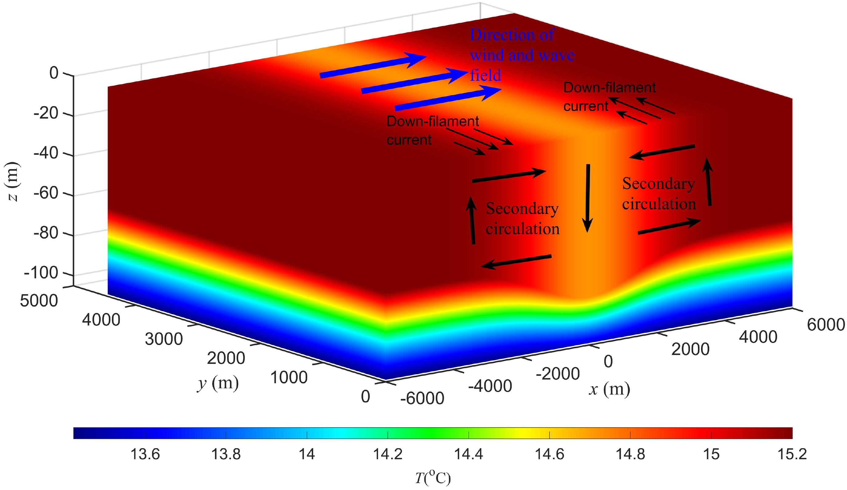
$ {\left\langle{w}\right\rangle}_{p}/{u}_{*} $ (the subscript p represents the “peak”) in the middle of the upper mixed layer z ≈ −30 m (McWilliams et al., 2015; Sullivan and McWilliams, 2018, 2019). Figure 2a shows a differentiation of the$ {\left\langle{w}\right\rangle}_{p}/{u}_{*} $ evolution forced by the different wind and wave fields indicated by$ {u}_{*}/fh $ . The results are unexpected and show that the negative and positive$ {\left\langle{w}\right\rangle}_{p}/{u}_{*} $ changes periodically with time. This result shows that, in the present simulations, the conventional conceptual model of the downwelling current (the negative$ \left\langle{w}\right\rangle/{u}_{*} $ ) and surface horizontal current$ \left\langle{{u}_{L}}\right\rangle/{u}_{*} $ ($ \left\langle{{u}_{L}}\right\rangle=\left\langle{u}\right\rangle+{u}_{s} $ is the Lagrange cross-filament current) convergence of a two-cell secondary circulation$ \left(\left\langle{{u}_{L}}\right\rangle,\left\langle{w}\right\rangle\right)/{u}_{*} $ for a cold filament (Gula et al., 2014; Hamlington et al., 2014; McWilliams et al., 2015) may transform into the upwelling current (the positive$ \left\langle{w}\right\rangle/{u}_{*} $ ) and surface horizontal current divergence within the lifecycle of cold filament frontogenesis. The change in secondary circulation directions may induce the conversion between the filament frontogenesis and frontolysis. This result is consistent with the theory that the vertical mixing suppresses the mixed layer instability (Crowe and Taylor, 2018). In addition, an enhancement in the wind and wave fields significantly reduces the minimum negative$ {\left\langle{w}\right\rangle}_{p}/{u}_{*} $ (Fig. 2b), implying that the levels of cold filament frontogenesis can be suppressed by the intense wind and wave fields.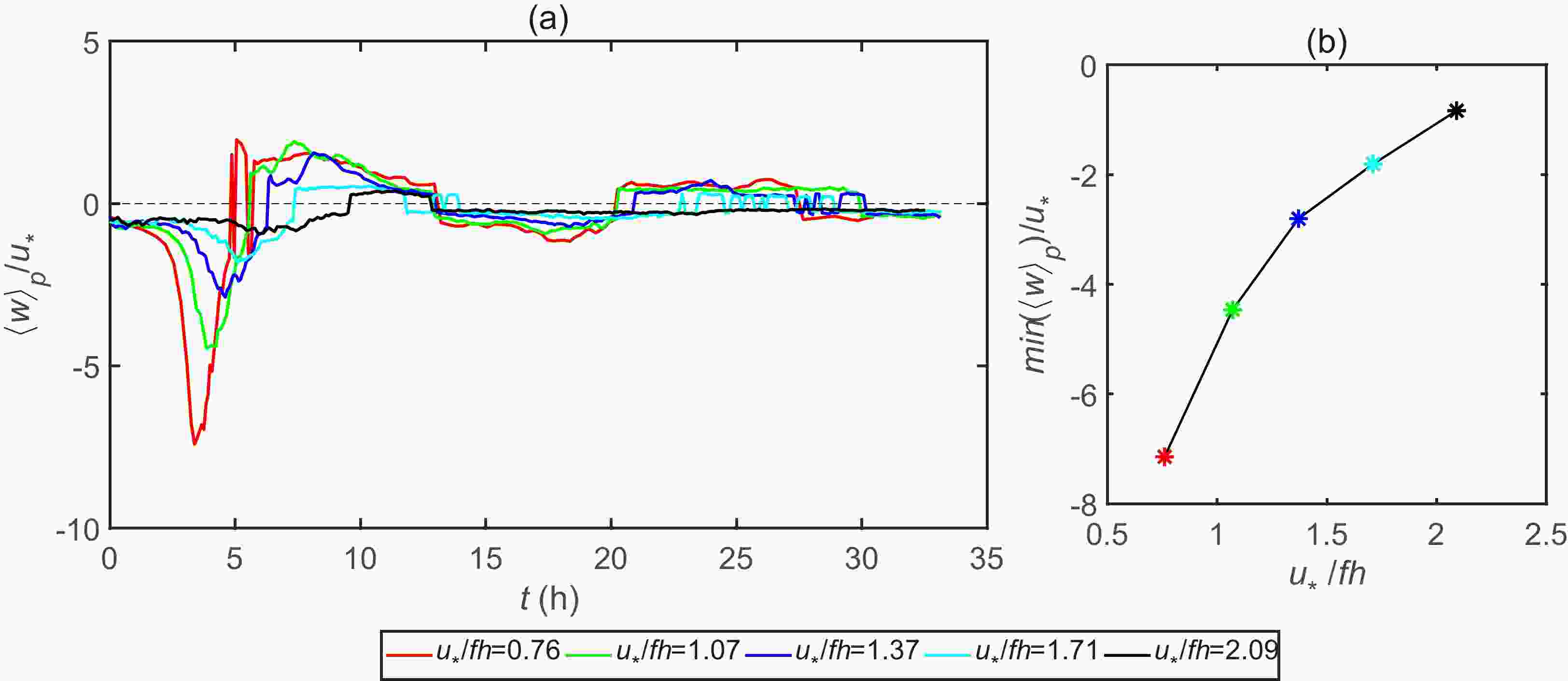
Figure 2. (a) Temporal variation of the normalized average peak vertical velocity
$ {\left\langle{w}\right\rangle}_{p}/{u}_{*} $ forced by the different wind and wave fields indicated by$ {u}_{*}/fh $ and (b) the variation of the minimum negative$ {\left\langle{w}\right\rangle}_{p}/{u}_{*} $ with a change of$ {u}_{*}/fh $ . The vertical dashed lines in (a) indicate the time for the change in the direction of the peak vertical velocity.The cross-filament (x-direction) profiles of the average cross-filament current (
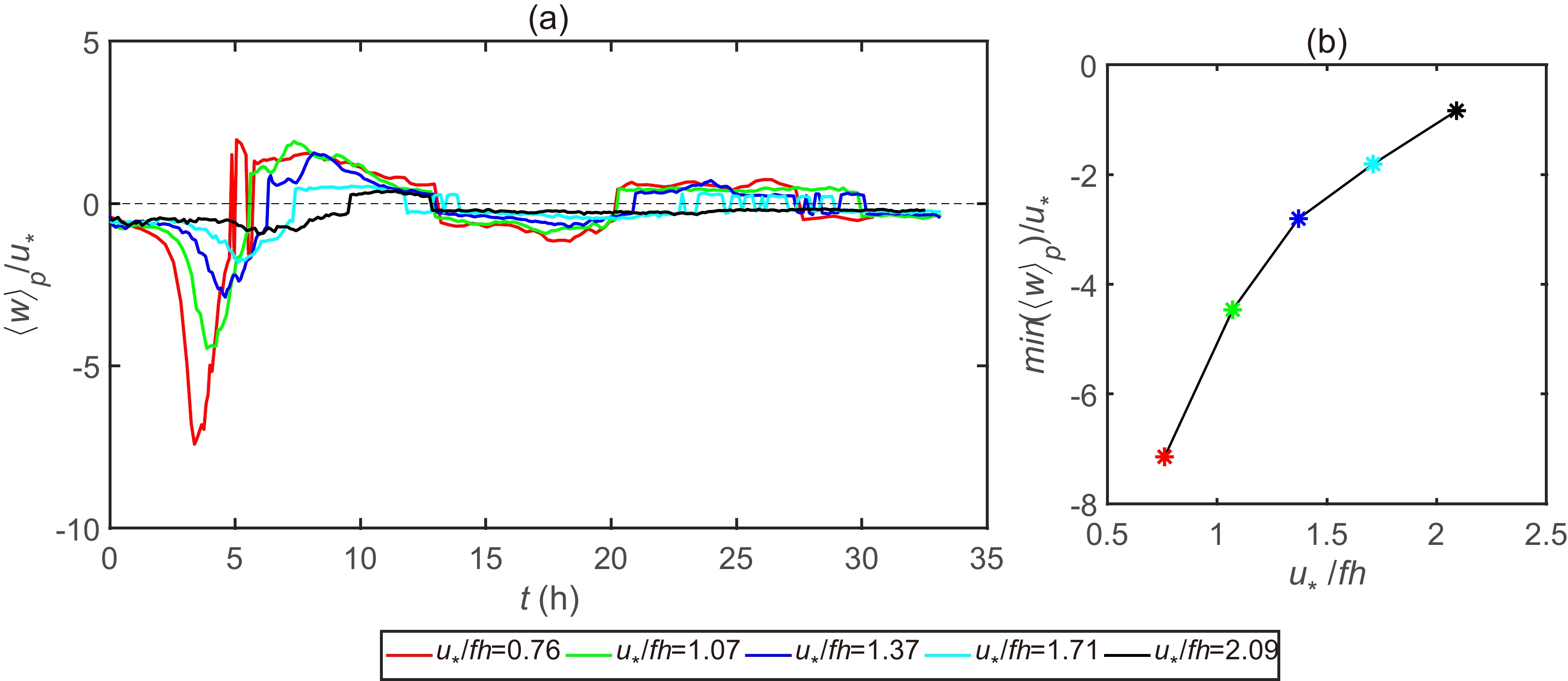
$ \left\langle{{u}_{L}}\right\rangle/{u}_{*} $ ), down-filament current ($ \left\langle{v}\right\rangle/{u}_{*} $ ), and temperature ($ \left\langle{{T}_{{\mathrm{so}}}-{T}_{{\mathrm{o}}}}\right\rangle/\delta {T}_{{\mathrm{o}}} $ ) in a near-surface layer are the important indicators for submesoscale currents of a cold filament impacted by different wind and wave fields (McWilliams et al., 2015; Sullivan and McWilliams, 2019). In order to smooth the statistics, the$ \left(\left\langle{{u}_{L}}\right\rangle,\left\langle{v}\right\rangle\right)/{u}_{*} $ and$ \left\langle{{T}_{{\mathrm{so}}}-{T}_{{\mathrm{o}}}}\right\rangle/\delta {T}_{{\mathrm{o}}} $ are averaged over a depth of −5 m < z < 0 (Sullivan and McWilliams, 2019). In particular, the peak vertical velocity$ {\left\langle{w}\right\rangle}_{p}/{u}_{\mathrm{*}} $ is near the middle of the upper mixed layer depth z ≈ −30 m. To highlight the intensity of the downwelling jet, the$ {\left\langle{w}\right\rangle}_{p}/{u}_{*} $ is not averaged over the depth.To further illustrate the impact of the different wind and wave fields on the levels of cold filament frontogenesis, Fig. 3 shows the cross-filament (x-direction) profiles of the average currents
$ \left(\left\langle{{u}_{L}}\right\rangle,\left\langle{v}\right\rangle,{\left\langle{w}\right\rangle}_{p}\right)/{u}_{*} $ and temperature$ \left\langle{T}_{{\mathrm{so}}}- {T}_{{\mathrm{o}}}\right\rangle/ \delta {T}_{{\mathrm{o}}} $ at the time stamp of the minimum negative$ {\left\langle{w}\right\rangle}_{p}/{u}_{*} $ (t = tmnw, the tmnw represents the time of the minimum negative$ {\left\langle{w}\right\rangle}_{p}/{u}_{*} $ ) (Fig. 2) forced by the different wind and wave fields. For the average horizontal currents$ \left(\left\langle{{u}_{L}}\right\rangle,\left\langle{v}\right\rangle\right)/{u}_{*} $ in a near-surface layer of depth 0 > z > −5 m (Figs. 3a and b), the left–right odd current symmetries are further disrupted with an increase of$ {u}_{*}/fh $ . Furthermore, when$ {u}_{*}/fh= $ 1.71 and 2.09, the horizontal currents have the same direction on the left and right flanks of the cold filament, suggesting that the submesoscale horizontal currents related to the TTW relation are exceeded by the horizontal currents created by the wind and wave fields in the remote fields of the cold filament. The enhancement of the disrupted left–right odd current symmetry for the cross-filament horizontal current$ \left\langle{{u}_{L}}\right\rangle/{u}_{*} $ causes a prominent decrease in both the average peak vertical velocity$ {\left\langle{w}\right\rangle}_{p}/{u}_{*} $ in the middle of the upper mixed layer z ≈ −30 m (Fig. 3c) and the average horizontal temperature gradient$ \left\langle{{T}_{{\mathrm{so}}}-{T}_{{\mathrm{o}}}}\right\rangle/{\delta T}_{{\mathrm{o}}} $ in a near-surface layer of depth 0 >$z $ > −5 m (Fig. 3d) (Sullivan and McWilliams, 2018). In addition, the positive$ \left\langle{{u}_{L}}\right\rangle/{u}_{*} $ on the right flank of the cold filament for$ {u}_{*}/fh= $ 1.71 and 2.09 illustrates that the cold water from the cold core can be advected to the right flank of the cold filament near the surface layer. This result shows that the magnitude of the wind and wave fields modulates the shape, magnitude and direction of the average currents (Figs. 3a–c) and temperature gradient (Fig. 3d) at t = tmnw.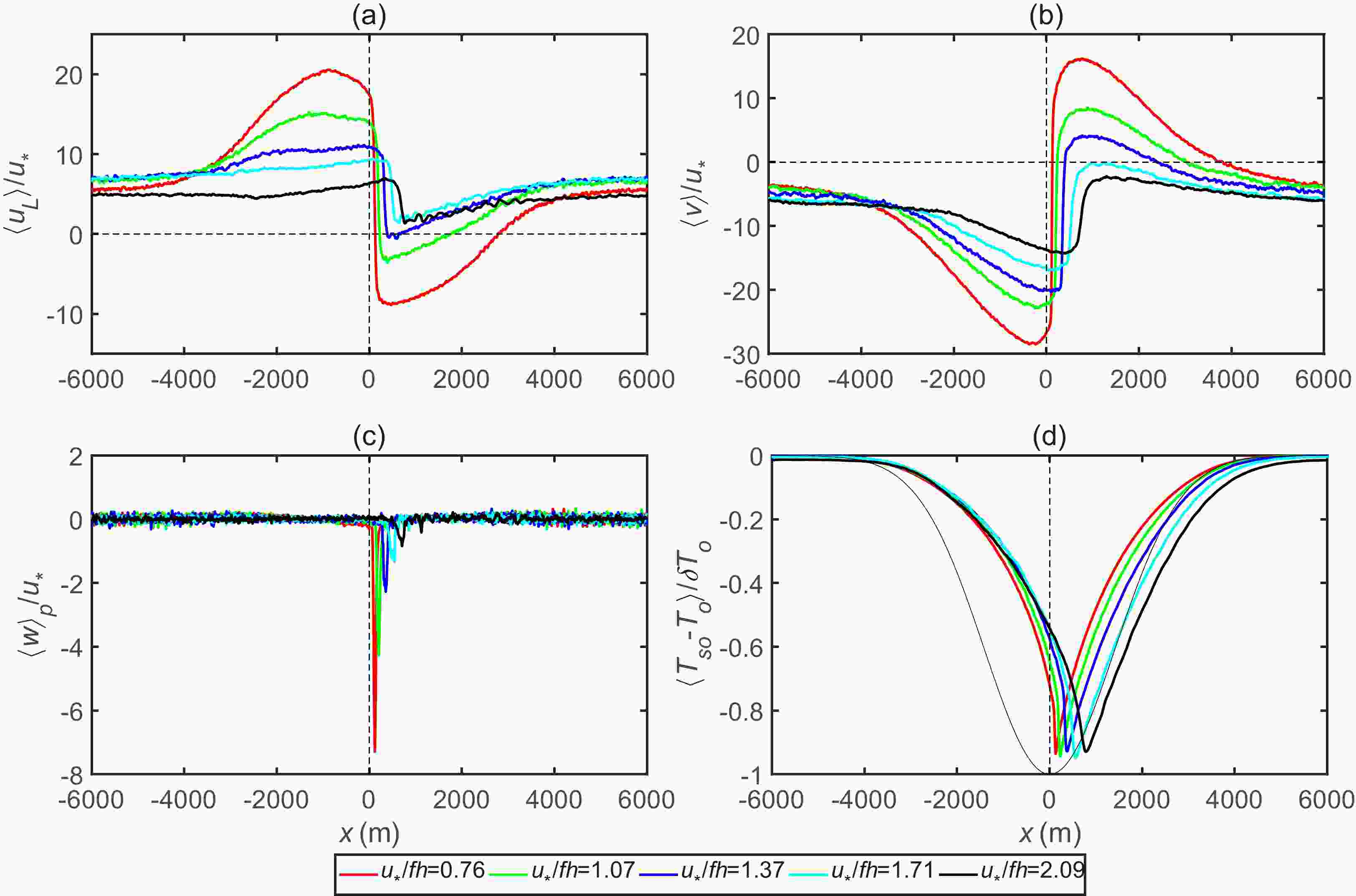
Figure 3. (a) Normalized average cross-filament current
$ \left\langle{{u}_{L}}\right\rangle/{u}_{*} $ and (b) normalized average down-filament current$ \left\langle{v}\right\rangle/{u}_{*} $ in a near-surface layer of depth −5 m < z < 0. (c) Normalized average peak vertical velocity$ {\left\langle{w}\right\rangle}_{p}/{u}_{*} $ in the middle of the upper mixed layer z ≈ −30 m and (d) normalized average temperature$ \left\langle{{T}_{{\mathrm{so}}}-{T}_{{\mathrm{o}}}}\right\rangle/{\delta T}_{{\mathrm{o}}} $ in a near-surface layer of depth −5 m < z < 0 forced by different wind and wave fields indicated by$ {u}_{*}/fh $ at t = tmnw. The fine black line in (d) is the initial temperature profile. -
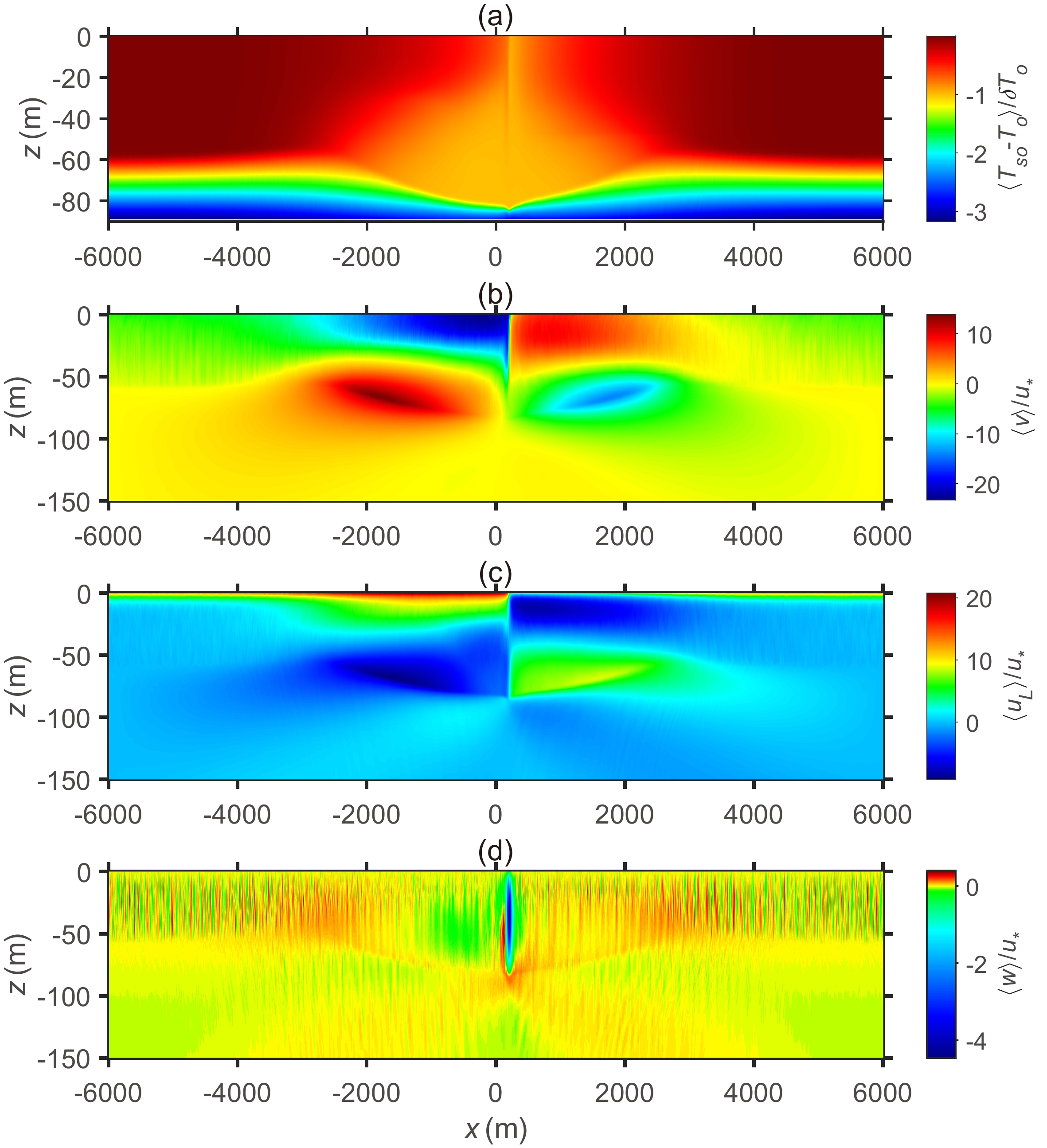
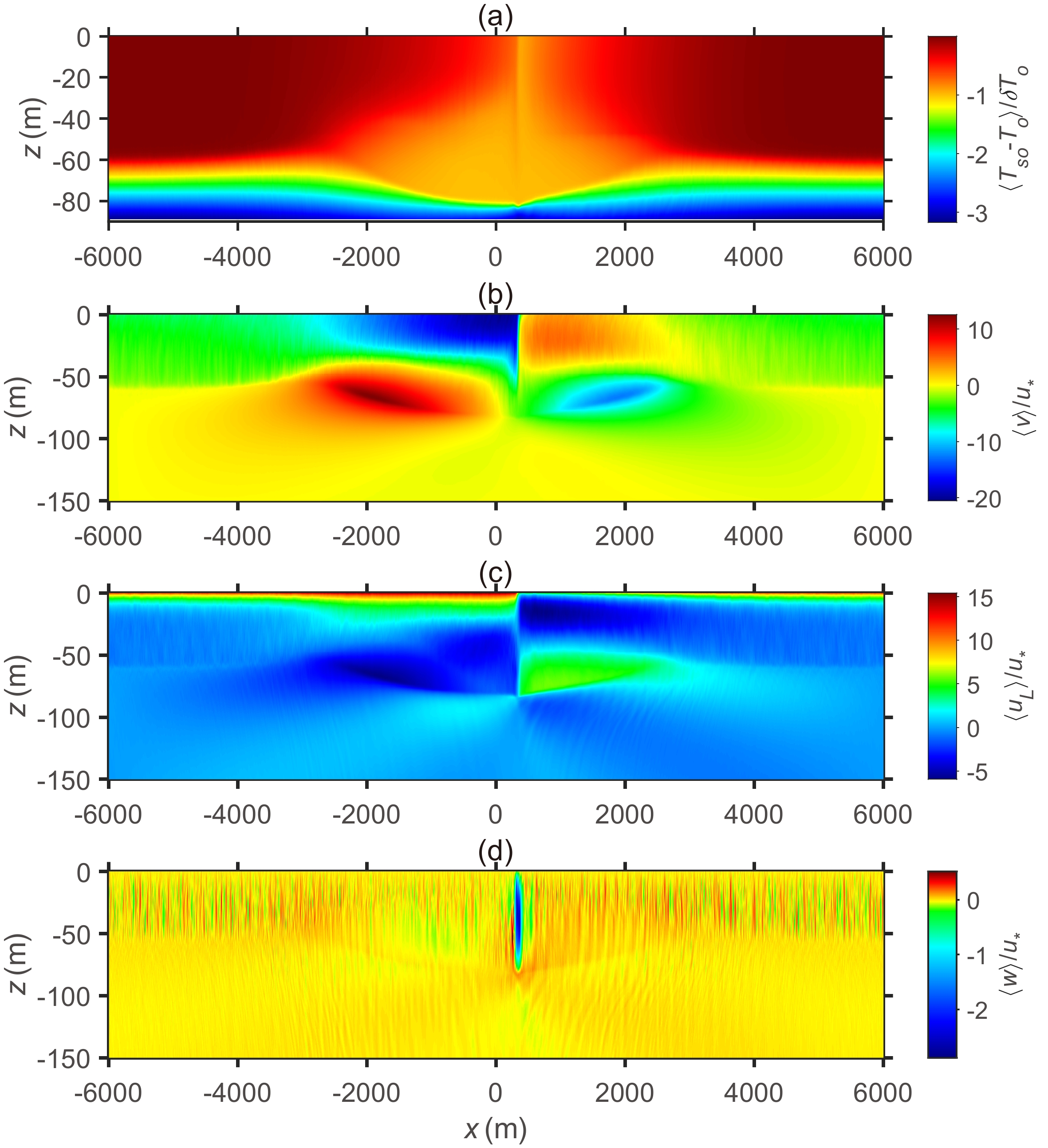
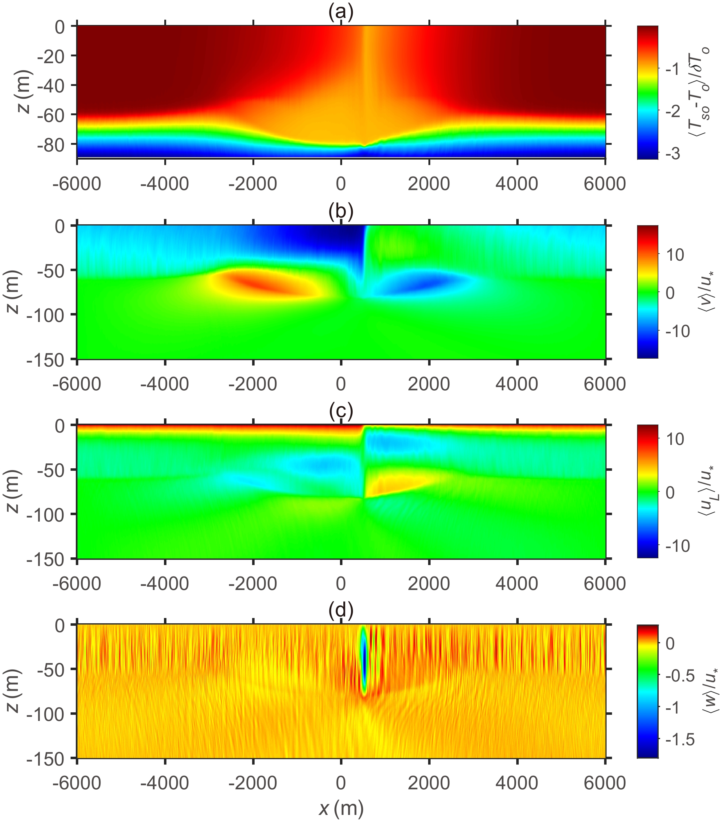
The variations of the flow structures forced by the different wind and wave fields in the interior of the upper mixed layer are one important aspect to parameterize the submesoscale currents (Hamlington et al., 2014; Suzuki et al., 2016; McWilliams, 2019, 2021). The average temperature and velocity fields
$ \left\langle{{T}_{{\mathrm{so}}}-{T}_{{\mathrm{o}}}}\right\rangle/{\delta T}_{{\mathrm{o}}} $ and$ \left(\left\langle{v}\right\rangle,\left\langle{{u}_{L}}\right\rangle,\left\langle{w}\right\rangle\right)/{u}_{*} $ forced by the different wind and wave fields at t = tmnw are shown in Figs. 4–8. The basic features of a two-cell secondary circulation—that is, the downwelling velocity in the zone of cold core and the opposing secondary circulation on the left and right sides of the cold core—are consistent with previous studies (Gula et al., 2014; McWilliams et al., 2015). However, the difference in the flow structures between this simulation and previous studies are also significant. The relatively warm water intrudes into the interior of the cold core on the left edge of the cold core, which induces the temperature gradient of the cross-filament direction on the left edge of the cold core to be significantly steeper than that on the right edge, irrespective of the magnitude of the wind and wave fields (Figs. 4a, 5a, 6a, 7a and 8a). This is partly similar to the previous result of Suzuki et al. (2016)—that is, a cold vertical wall of the temperature field appeared on the right side of the front. The reason is that the$ \left\langle{{u}_{L}}\right\rangle/{u}_{*} $ is positive (negative) for the upper branch of the left (right) secondary circulation (Figs. 4c, 5c, 6c, 7c and 8c) for this simulation with the cross-filament wind and wave fields, and the Stokes shear force$ {S}_{\mathrm{s}\mathrm{f}}=-{u}_{L}\partial {u}_{\mathrm{s}}/\partial z $ [the same (opposite) direction between the wave and current creates (suppresses) the downwelling current] (Suzuki and Fox-Kemper, 2016) enhances the strength of the downwelling current on the left edge of the cold core by a superposition of the downwelling currents induced by the Stokes shear force and the secondary circulations, respectively. The enhanced strength of the positive$ \left\langle{{u}_{L}}\right\rangle/{u}_{*} $ for the upper branch of the left secondary circulation caused by the wind and wave fields also plays an important role in the warm water including the interior of the cold core, because the convergence of the horizontal current may be strengthened by the larger amount of water flowing toward the filament center on the left flank of the cold filament. The flow visualization does show that the downwelling current on the left edge of the cold core is significantly stronger than elsewhere in the cold core.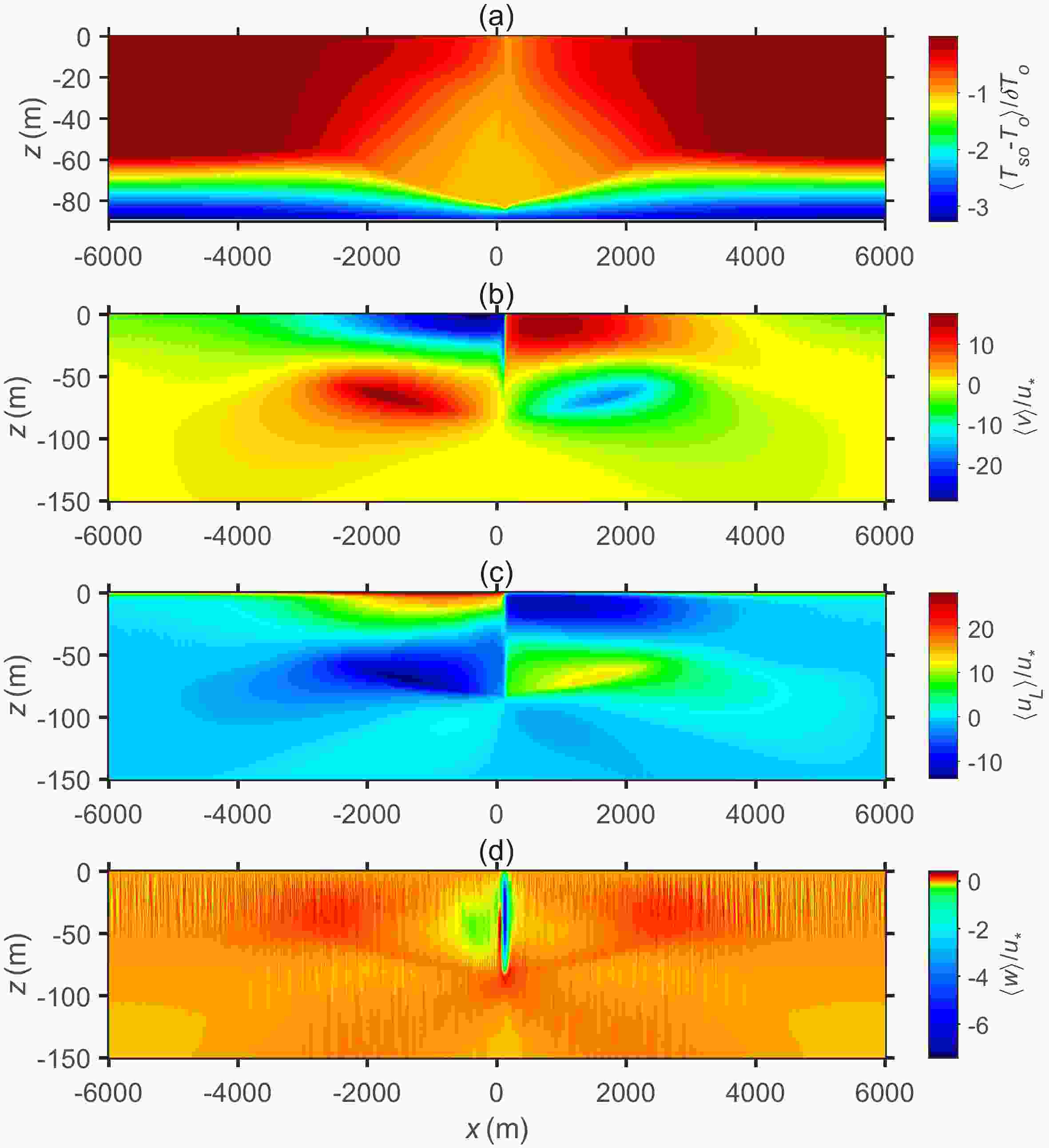
Figure 4. The normalized average fields of (a) the temperature
$ \left\langle{{T}_{{\mathrm{so}}}-{T}_{{\mathrm{o}}}}\right\rangle/{\delta T}_{{\mathrm{o}}} $ , (b) the down-filament velocity$ \left\langle{v}\right\rangle/{u}_{*} $ , (c) the cross-filament velocity$ \left\langle{{u}_{L}}\right\rangle/{u}_{*} $ , and (d) the vertical velocity$ \left\langle{w}\right\rangle/{u}_{*} $ for$ {u}_{*}/fh $ = 0.76 at tmnw = 3.37 h.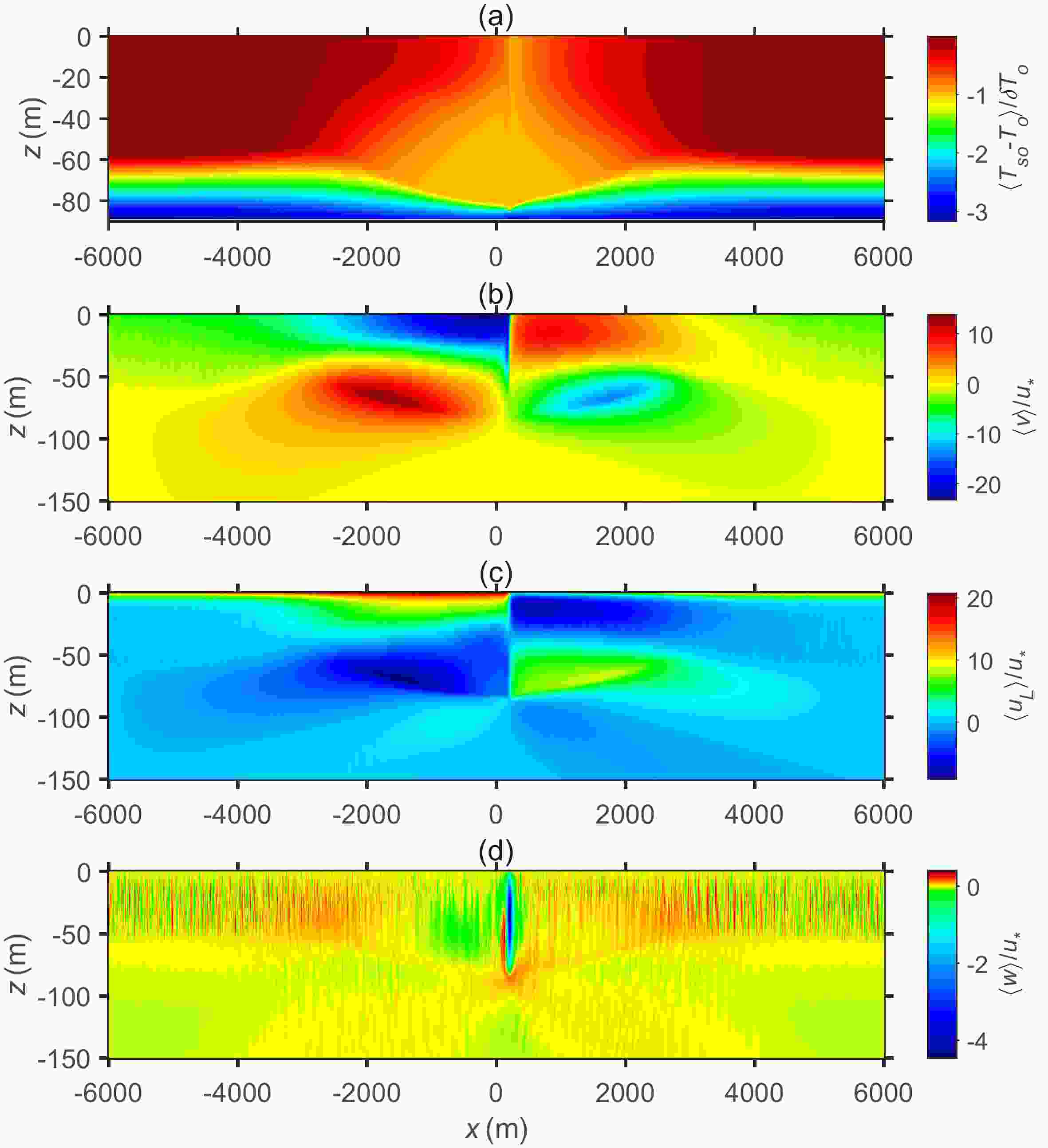
Figure 5. The normalized average fields of (a) the temperature
$ \left\langle{{T}_{{\mathrm{so}}}-{T}_{{\mathrm{o}}}}\right\rangle/{\delta T}_{{\mathrm{o}}} $ , (b) the down-filament velocity$ \left\langle{v}\right\rangle/{u}_{*} $ , (c) the cross-filament velocity$ \left\langle{{u}_{L}}\right\rangle/{u}_{*} $ , and (d) the vertical velocity$ \left\langle{w}\right\rangle/{u}_{*} $ for$ {u}_{*}/fh $ = 1.07 at tmnw = 3.86 h.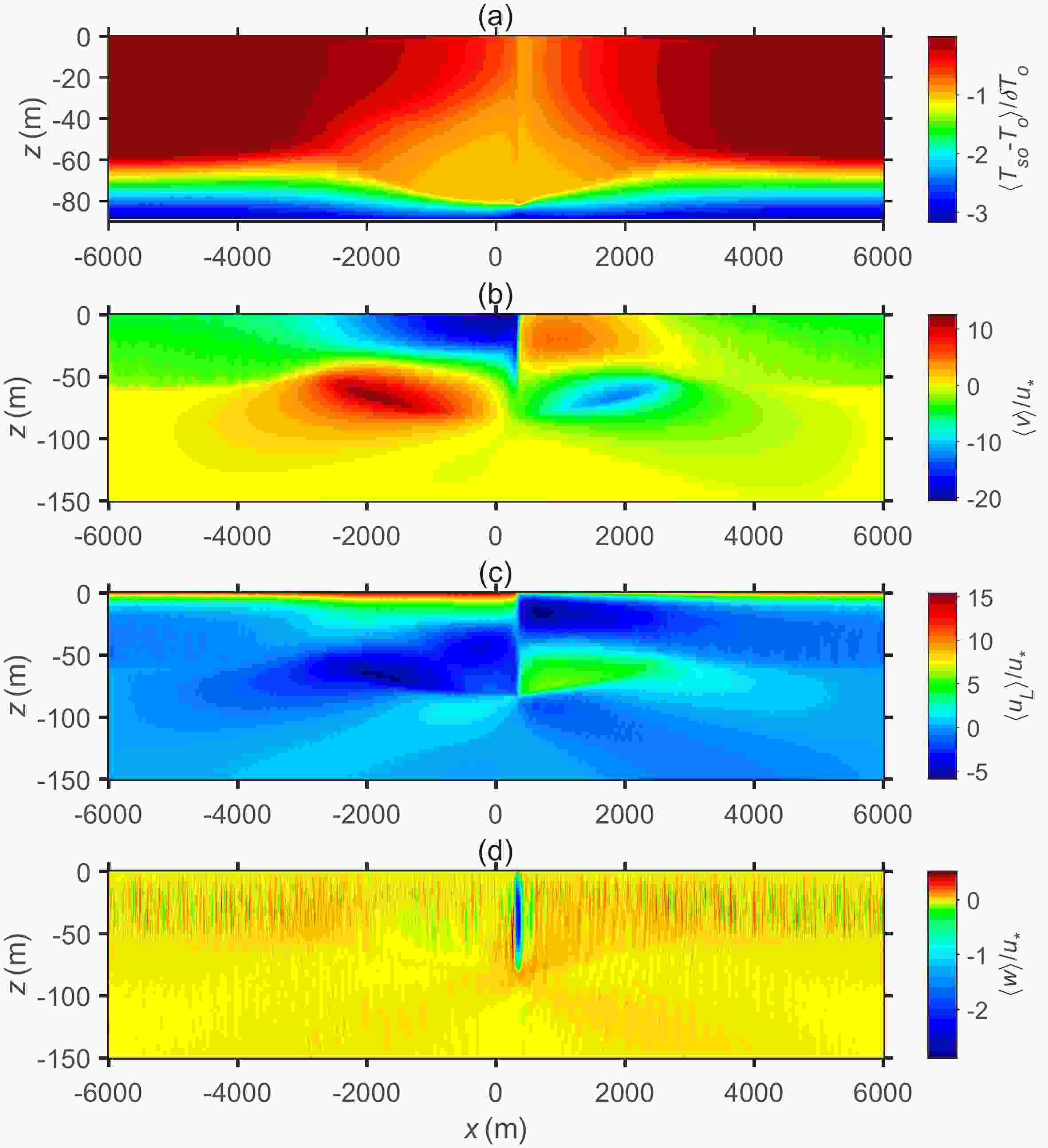
Figure 6. The normalized average fields of (a) the temperature
$ \left\langle{{T}_{{\mathrm{so}}}-{T}_{{\mathrm{o}}}}\right\rangle/{\delta T}_{{\mathrm{o}}} $ , (b) the down-filament velocity$ \left\langle{v}\right\rangle/{u}_{*} $ , (c) the cross-filament velocity$ \left\langle{{u}_{L}}\right\rangle/{u}_{*} $ , and (d) the vertical velocity$ \left\langle{w}\right\rangle/{u}_{*} $ for$ {u}_{*}/fh $ = 1.37 at tmnw = 4.61 h.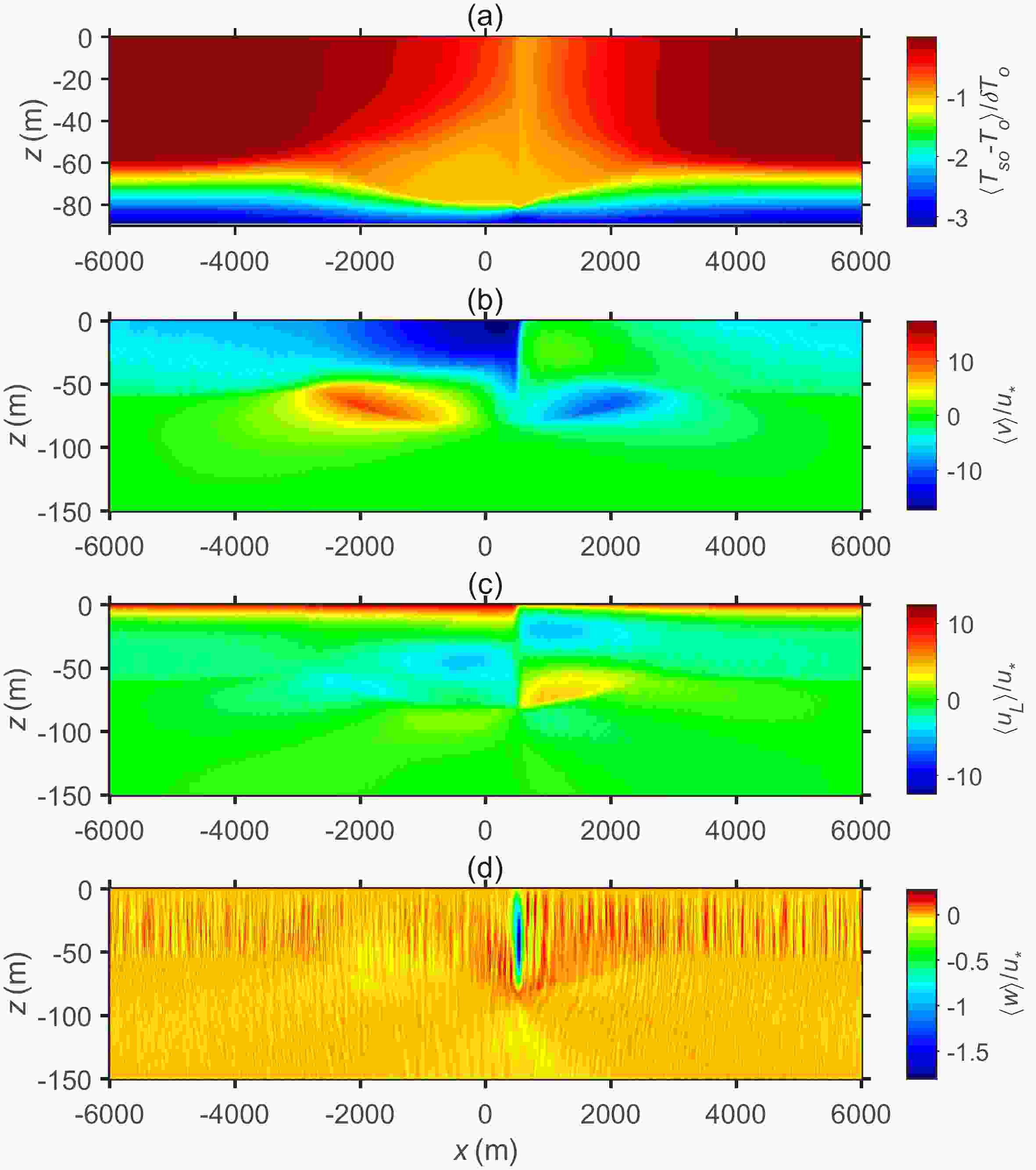
Figure 7. The normalized average fields of (a) the temperature
$ \left\langle{{T}_{{\mathrm{so}}}-{T}_{{\mathrm{o}}}}\right\rangle/{\delta T}_{{\mathrm{o}}} $ , (b) the down-filament velocity$ \left\langle{v}\right\rangle/{u}_{*} $ , (c) the cross-filament velocity$ \left\langle{{u}_{L}}\right\rangle/{u}_{*} $ , and (d) the vertical velocity$ \left\langle{w}\right\rangle/{u}_{*} $ for$ {u}_{*}/fh $ = 1.71 at tmnw = 5.13 h.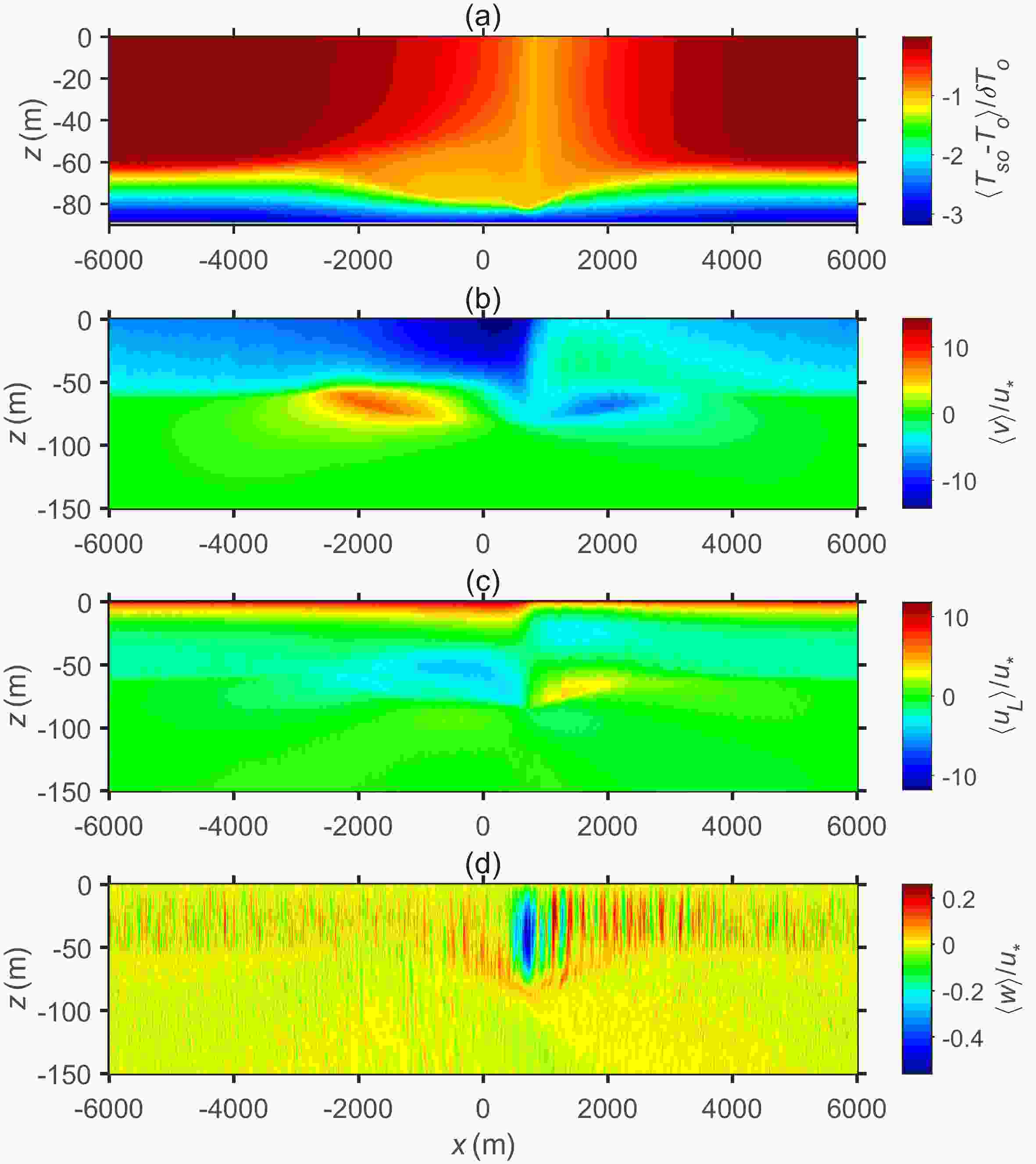
Figure 8. The normalized average fields of (a) the temperature
$ \left\langle{{T}_{{\mathrm{so}}}-{T}_{{\mathrm{o}}}}\right\rangle/{\delta T}_{{\mathrm{o}}} $ , (b) the down-filament velocity$ \left\langle{v}\right\rangle/{u}_{*} $ , (c) the cross-filament velocity$ \left\langle{{u}_{L}}\right\rangle/{u}_{*} $ , and (d) the vertical velocity$ \left\langle{w}\right\rangle/{u}_{*} $ for$ {u}_{*}/fh $ = 2.09 at tmnw = 7.42 h.Next, we analyze the impact of the different wind and wave fields on the flow structures in the interior of the upper mixed layer. With an increment of the wind and wave fields, the odd symmetry of
$ \left\langle{v}\right\rangle/{u}_{*} $ (Figs. 4b, 5b, 6b, 7b and 8b) and$ \left\langle{{u}_{L}}\right\rangle/{u}_{*} $ (Figs. 4c, 5c, 6c, 7c and 8c) is notably broken, which distorts the even symmetry of$ \left\langle{{T}_{\mathrm{s}\mathrm{o}}-{T}_{\mathrm{o}}}\right\rangle/{\delta T}_{\mathrm{o}} $ (Figs. 4a, 5a, 6a, 7a and 8a). This intense asymmetry is mainly due to the fact that the cross- and down-filament currents caused by an increase in the wind and wave fields gradually exceed the opposite submesoscale cross- and down-filament currents on the right side of the cold core related to the TTW relation near the surface layer, as shown in Figs. 4c, 5c, 6c, 7c and 8c, and Fig. 3, and the weakened temperature gradient with an increase in the wind and wave fields (Figs. 3a, 4a, 5a, 6a and 7a) also reduces the down-filament currents (Figs. 4b, 5b, 6b, b and 8b) based on the TTW relation [Eq. (1)], which is partly consistent with the diagnostic analysis of McWilliams (2018). The enhancement of the horizontal current asymmetries with an increase in the wind and wave fields may further suppress the level of cold filament frontogenesis (Suzuki and Fox-Kemper, 2016; McWilliams, 2018), which induces the decay of both the sharpening gradient of the temperature fields above z = −10 m (Figs. 4a, 5a, 6a, 7a and 8a) and the amplitude of the vertical velocity (Figs. 4d, 5d, 6d, 7d and 8d). -
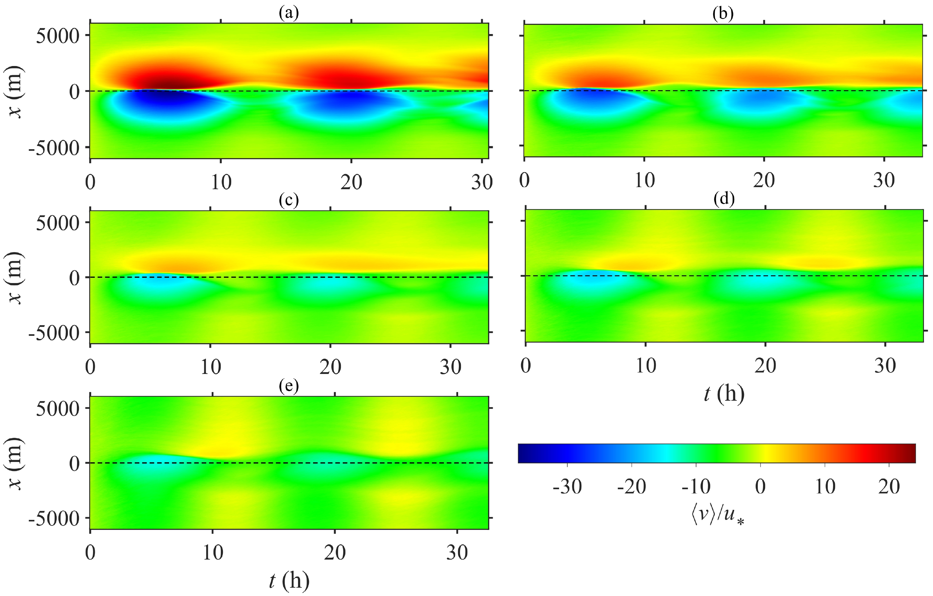
To dig deeper into the impact of the magnitude of the wind and wave fields on the frontogenetic trend of cold filament, we next compare the variations of the average horizontal currents
$ \left(\left\langle{{u}_{L}}\right\rangle,\left\langle{v}\right\rangle\right)/{u}_{*} $ in a near-surface layer of depth 0 > z > −5 m forced by the different wind and wave fields (Figs. 9 and 10). The left–right odd current symmetries of the$ \left(\left\langle{{u}_{L}}\right\rangle,\left\langle{v}\right\rangle\right)/{u}_{*} $ are further broken by the enhancement in the wind and wave fields, despite the periodic variation of the$ \left(\left\langle{{u}_{L}}\right\rangle,\left\langle{v}\right\rangle\right)/{u}_{*} $ amplitude with time being controlled by the inertial oscillation and the$ \left(\left\langle{{u}_{L}}\right\rangle,\left\langle{v}\right\rangle\right)/{u}_{*} $ amplitude having a reduced trend with time independent of the magnitude of the wind and wave fields (Figs. 9 and 10). This reduced trend of the$ \left(\left\langle{{u}_{L}}\right\rangle,\left\langle{v}\right\rangle\right)/{u}_{*} $ amplitude with time is mainly created by the increase in stratification suppressing the cross-filament vertical momentum flux (not shown) and the decrease in the temperature gradient (Fig. 12) with time based on the TTW relation [Eqs. (1) and (2)]. The periodic variation in the magnitude of the along-filament currents with time (Fig. 9) is similar with the model results of Shakespeare and Taylor (2013). Moreover, for$ {u}_{*}/fh $ = 1.71 and 2.09 (Figs. 9d and 9e), the$ \left\langle{{u}_{L}}\right\rangle/{u}_{*} $ is always a positive value on the left and right flanks of the cold filament within this simulation time, indicating that the positive cross-filament current created by the wind and wave fields is always larger than the opposite submesoscale cross-filament current related to the TTW relation. Noticeably, for$ {u}_{*}/fh $ = 0.76, 1.07 and 1.37 (Figs. 9a–c), the periodic change in the direction of$ \left\langle{{u}_{L}}\right\rangle/{u}_{*} $ on the left and right flanks of the cold filament with time is controlled by the inertial oscillation, showing that the convergence and divergence of the surface horizontal current—that is, the direction of secondary circulations—is the periodic change associated with the inertial period ($ 2\pi /f\approx $ 14 h). The convergence and divergence of$ \left\langle{{u}_{L}}\right\rangle/{u}_{*} $ are a key indicator for the frontogenesis and frontolysis of a cold filament.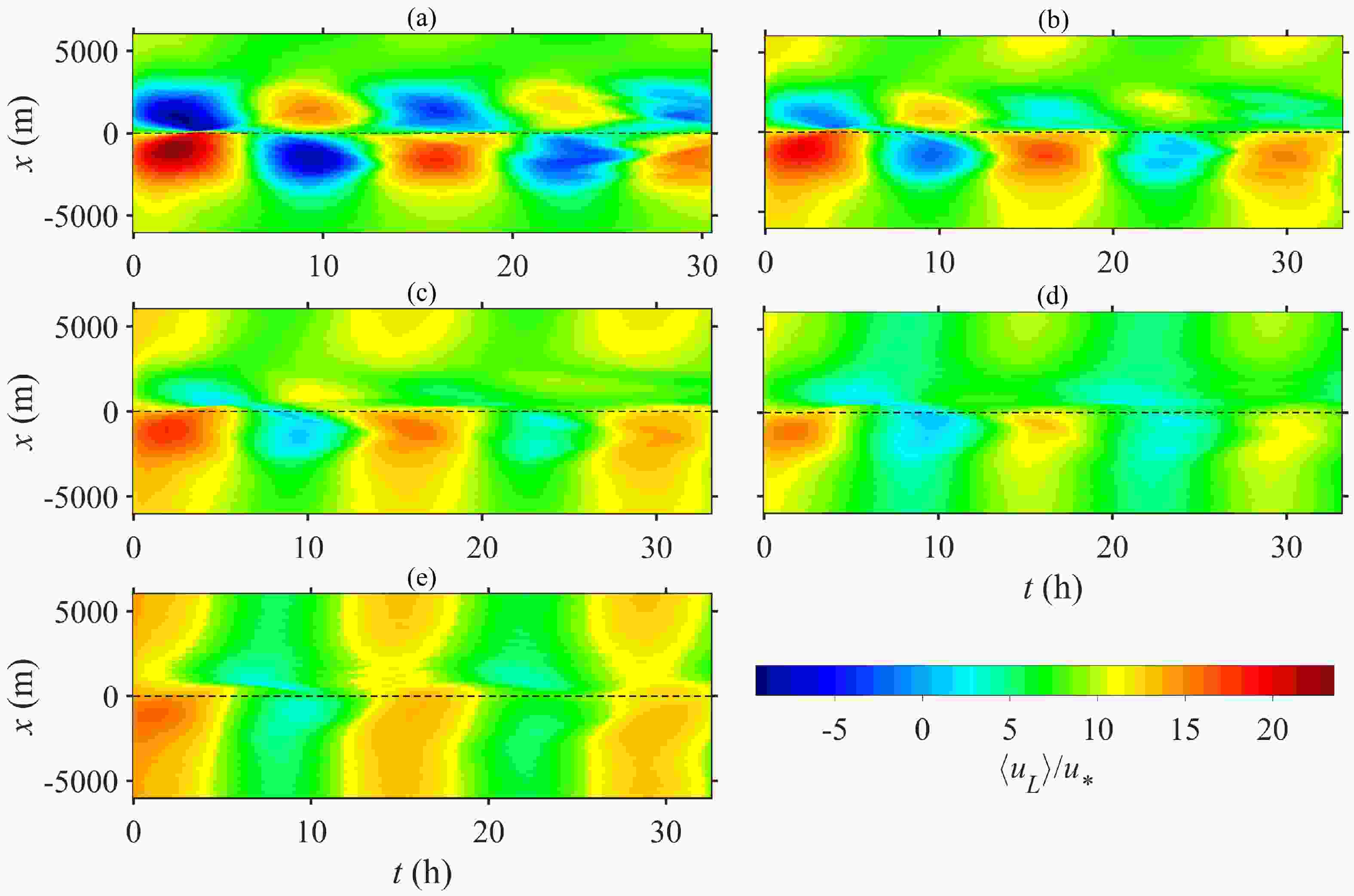
Figure 9. Temporal variation of the normalized average cross-filament current
$ \left\langle{{u}_{L}}\right\rangle/{u}_{*} $ in a near-surface layer of depth −5 m < z < 0 of (a)$ {u}_{*}/fh $ = 0.76, (b)$ {u}_{*}/fh $ = 1.07, (c)$ {u}_{*}/fh $ = 1.37, (d)$ {u}_{*}/fh $ = 1.71, and (e)$ {u}_{*}/fh $ = 2.09.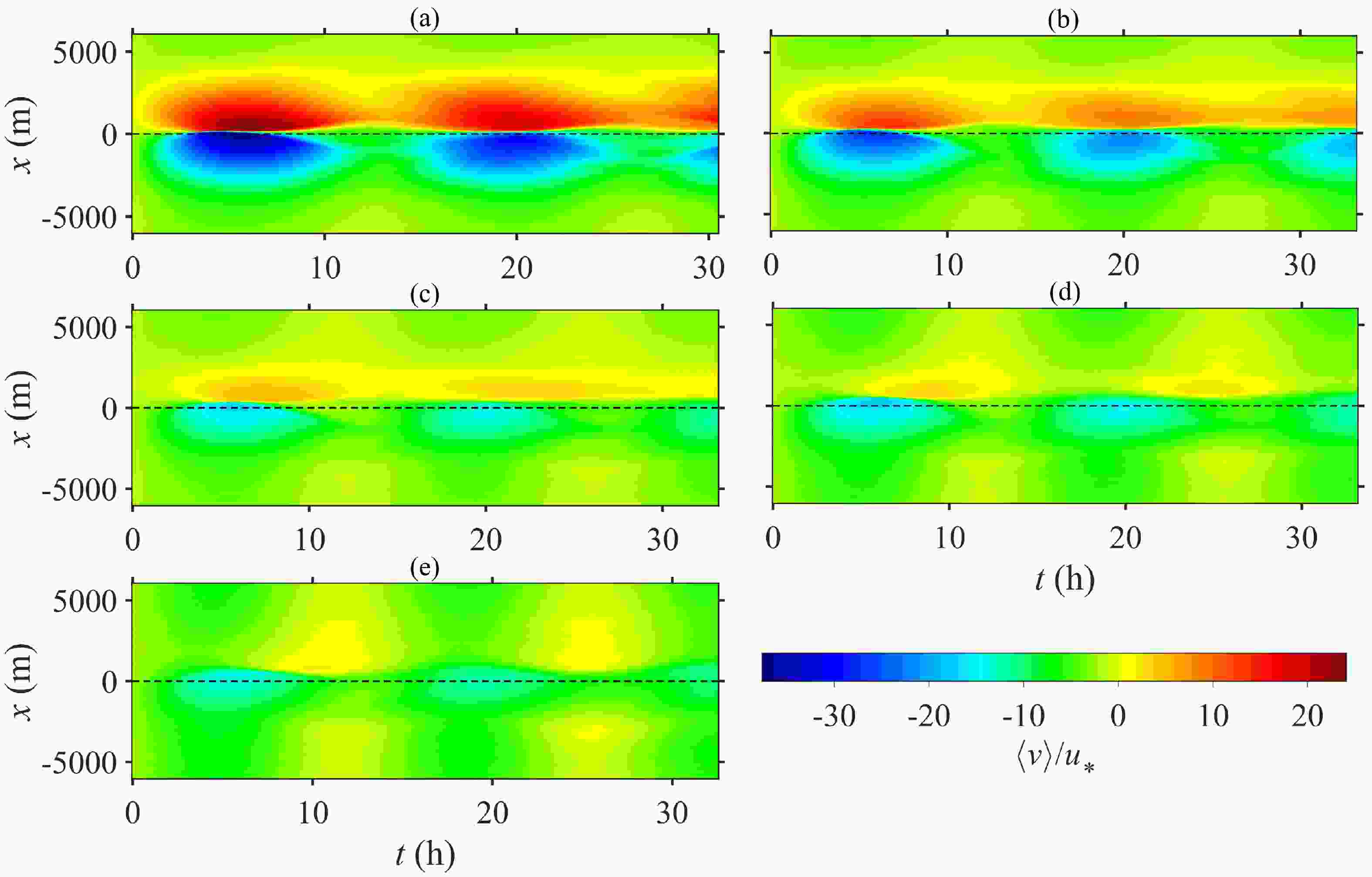
Figure 10. Temporal variation of the normalized average cross-filament current
$ \left\langle{v}\right\rangle/{u}_{*} $ in a near-surface layer of depth −5 m < z < 0 of (a)$ {u}_{*}/fh $ = 0.76, (b)$ {u}_{*}/fh $ = 1.07, (c)$ {u}_{*}/fh $ = 1.37, (d)$ {u}_{*}/fh $ = 1.71, and (e)$ {u}_{*}/fh $ = 2.09.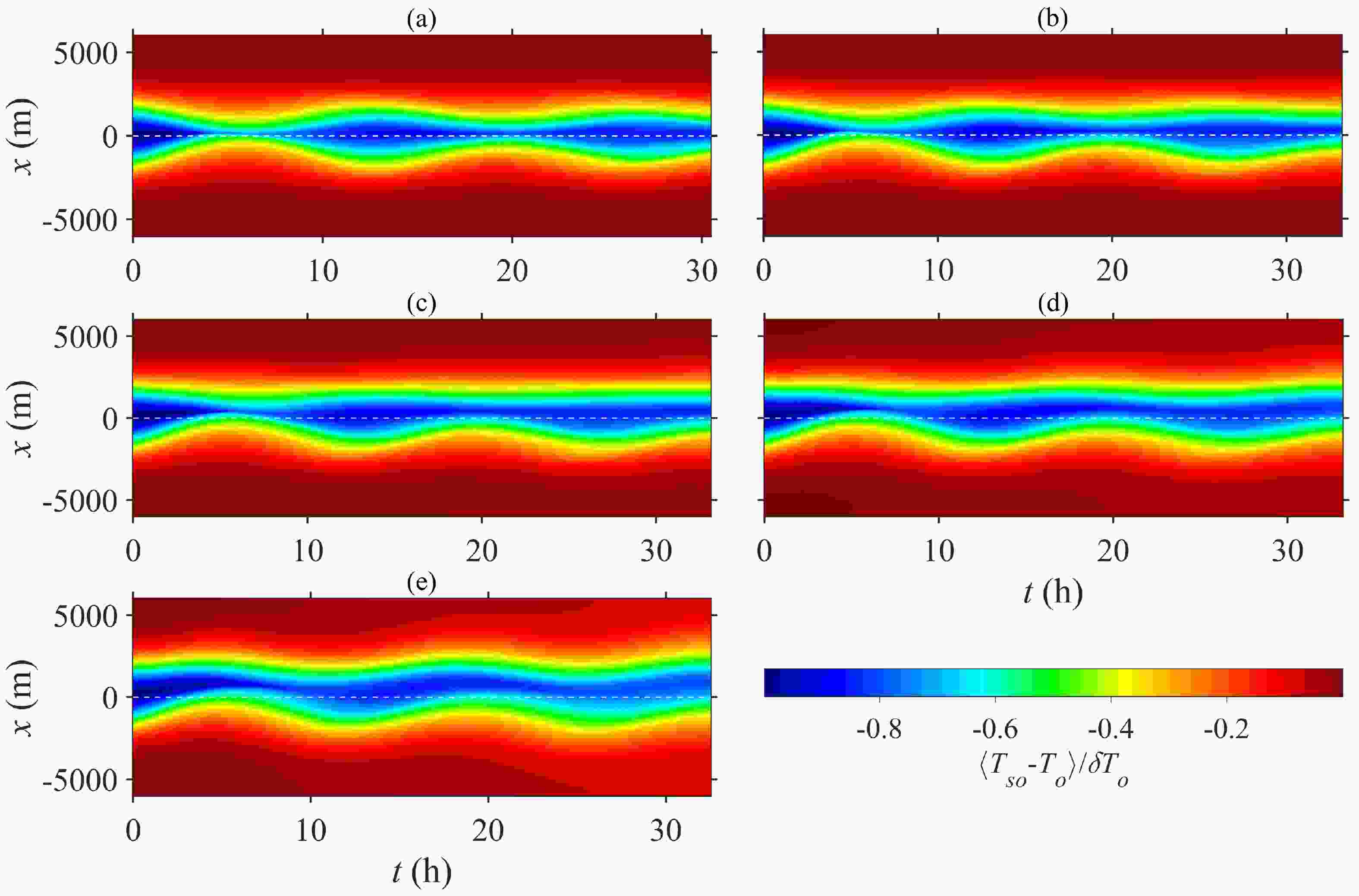
Figure 12. Temporal variation of the normalized average cross-filament temperature
$ \left\langle{{T}_{\mathrm{s}\mathrm{o}}-{T}_{\mathrm{o}}}\right\rangle/{\delta T}_{\mathrm{o}} $ in a near-surface layer of depth −5 m < z < 0 of (a)$ {u}_{*}/fh $ = 0.76, (b)$ {u}_{*}/fh $ = 1.07, (c)$ {u}_{*}/fh $ = 1.37, (d)$ {u}_{*}/fh $ = 1.71, and (e)$ {u}_{*}/fh $ = 2.09.The magnitude and direction of the average peak vertical velocity
$ {\left\langle{w}\right\rangle}_{p}/{u}_{*} $ in the middle of the upper mixed layer, z ≈ −30 m, is an important signature for the levels and states of the filament frontogenesis and frontolysis (McWilliams et al., 2015; McWilliams, 2017). The width of the cold core indicated by the temperature$ \left\langle{{T}_{\mathrm{s}\mathrm{o}}-{T}_{\mathrm{o}}}\right\rangle/\delta {T}_{\mathrm{o}} $ in a near-surface layer of depth 0 > z > −5 m is also an informative metric for the states of filament frontogenesis and frontolysis (Hamlington et al., 2014; McWilliams, 2016). The temporal variations of$ {\left\langle{w}\right\rangle}_{p}/{u}_{*} $ and$ \left\langle{{T}_{\mathrm{s}\mathrm{o}}-{T}_{\mathrm{o}}}\right\rangle/\delta {T}_{\mathrm{o}} $ forced by the different wind and wave fields are shown in Figs. 11 and 12, respectively. The amplitude of$ {\left\langle{w}\right\rangle}_{p}/{u}_{*} $ decays (Fig. 11) and the width of the cold core enlarges (Fig. 12) with an increase of$ {u}_{*}/fh $ , which is due to an enhancement in the asymmetry of$ \left\langle{{u}_{L}}\right\rangle/{u}_{*} $ (Fig. 9) possibly suppressing the level of cold filament frontogenesis (Sullivan and McWilliams, 2019). The change in the amplitude and direction of$ {\left\langle{w}\right\rangle}_{p}/{u}_{*} $ with time (Fig. 11) is modulated by that of$ \left\langle{{u}_{L}}\right\rangle/{u}_{*} $ , which is controlled by the inertial oscillation (Fig. 9), showing that the lifecycle of cold filament frontogenesis includes the processes of filament frontogenesis and frontolysis. Moreover, the amplitude of the downwelling current (negative$ {\left\langle{w}\right\rangle}_{p}/{u}_{*} $ ) is much larger than that of the upwelling current (positive$ {\left\langle{w}\right\rangle}_{p}/{u}_{*} $ ), which indicates that the level of filament frontogenesis is stronger than that of filament frontolysis (shown in Fig. 15 of section 4). The change in the width of the cold core with time is the periodic shrinkage–expansion (Fig. 12) caused by the filament frontogenesis and frontolysis indicated by the surface convergence and divergence of the cross-filament current with the downwelling and upwelling current in the zone of the cold core (Figs. 9 and 11)—that is, the filament frontogenesis and frontolysis sharpen and smooth the gradient of the temperature and horizontal currents, respectively. These results demonstrate that the lifecycle of cold filament frontogenesis will involve multiple stages of filament frontogenesis and frontolysis, which indicates that the simple conception of cold filament frontogenesis including only the onset, arrest, decay and broken periods (McWilliams, 2016, 2021) is not suitable for the simulation cases considered here. In addition, the varied range of the right edge of the cold core with time reduces as$ {u}_{*}/fh $ changes from 0.76 to 1.37 (Figs. 12a–c) and increase as$ {u}_{*}/fh $ changes from 1.37 to 2.09 (Figs. 12c–e), owing to the fact that the enhancement in the cross-filament current created by an increase in the wind and wave fields changes from smaller to larger than the opposite secondary current associated with the TTW relation on the right side of the cold core when$ {u}_{*}/fh $ varies from$ {u}_{*}/fh $ < 1.37 to$ {u}_{*}/fh $ > 1.37 (Fig. 10).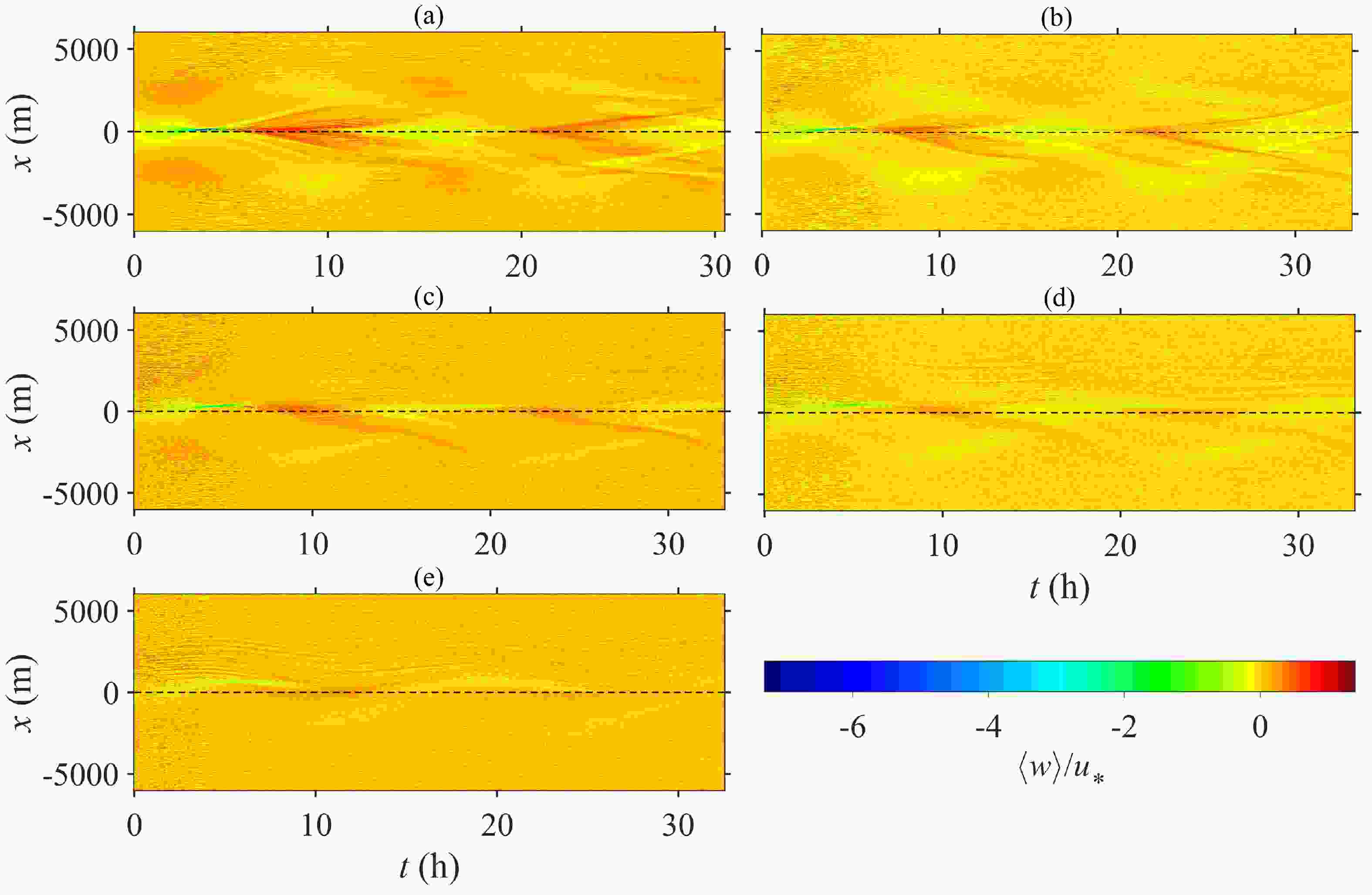
Figure 11. Temporal variation of the normalized average peak vertical current
$ {\left\langle{w}\right\rangle}_{p}/{u}_{*} $ in the middle of the upper mixed layer (z ≈ −30 m) of (a)$ {u}_{*}/fh $ = 0.76, (b)$ {u}_{*}/fh $ = 1.07, (c)$ {u}_{*}/fh $ = 1.37, (d)$ {u}_{*}/fh $ = 1.71, and (e)$ {u}_{*}/fh $ = 2.09.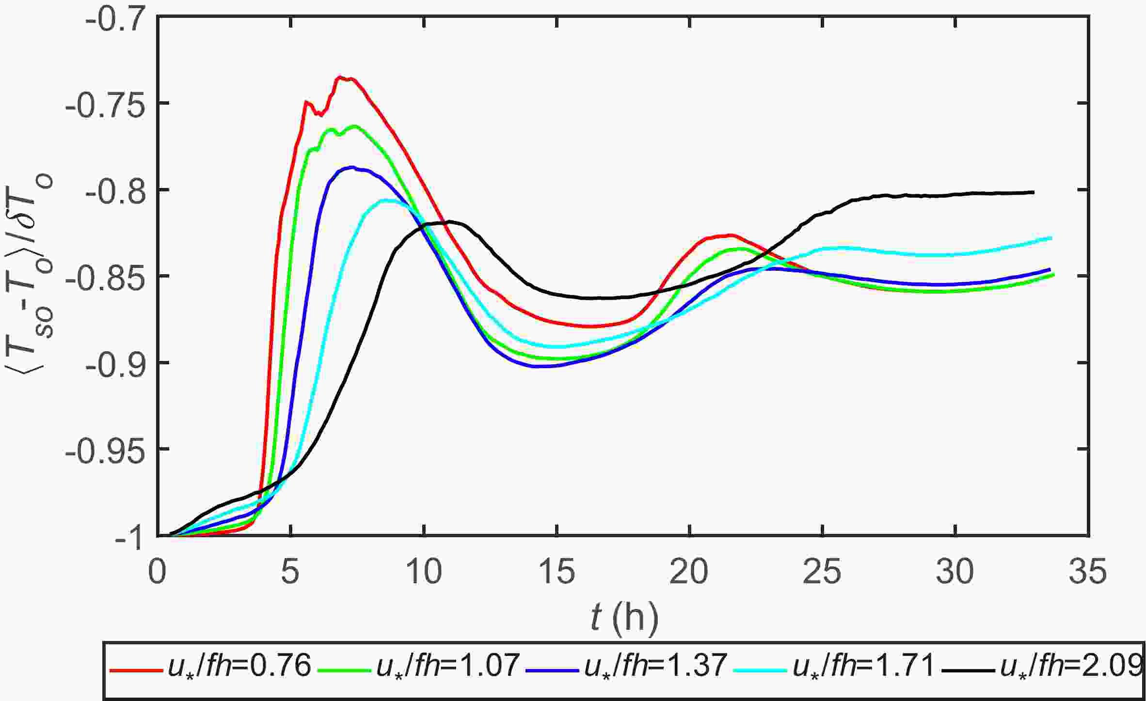
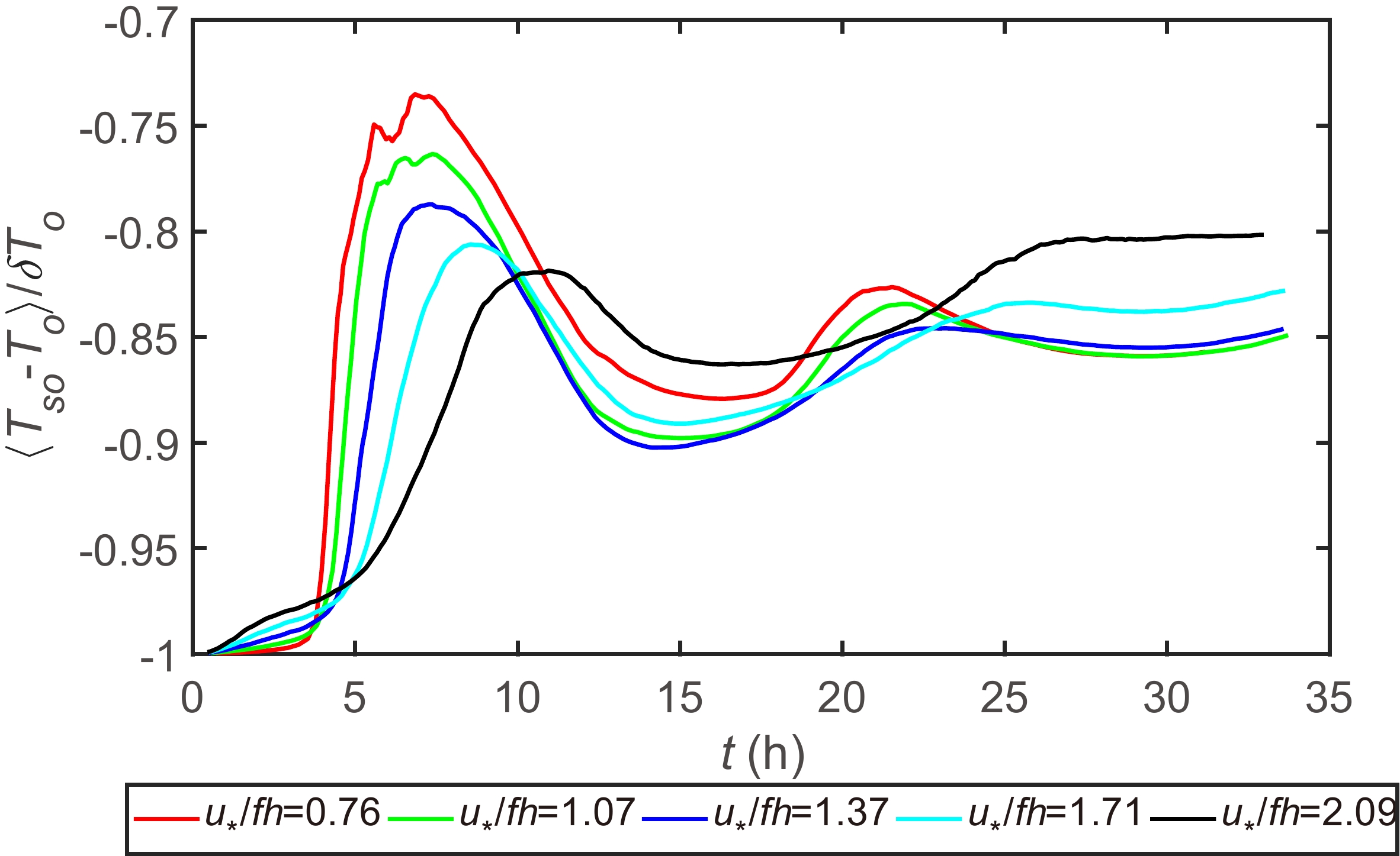
Figure 15. Temporal variation of the normalized average temperature
$ \left\langle{{T}_{\mathrm{s}\mathrm{o}}-{T}_{\mathrm{o}}}\right\rangle/{\delta T}_{\mathrm{o}} $ of the cold core center in a near-surface layer of depth −5 m < z < 0 with a change of$ {u}_{*}/fh $ . -
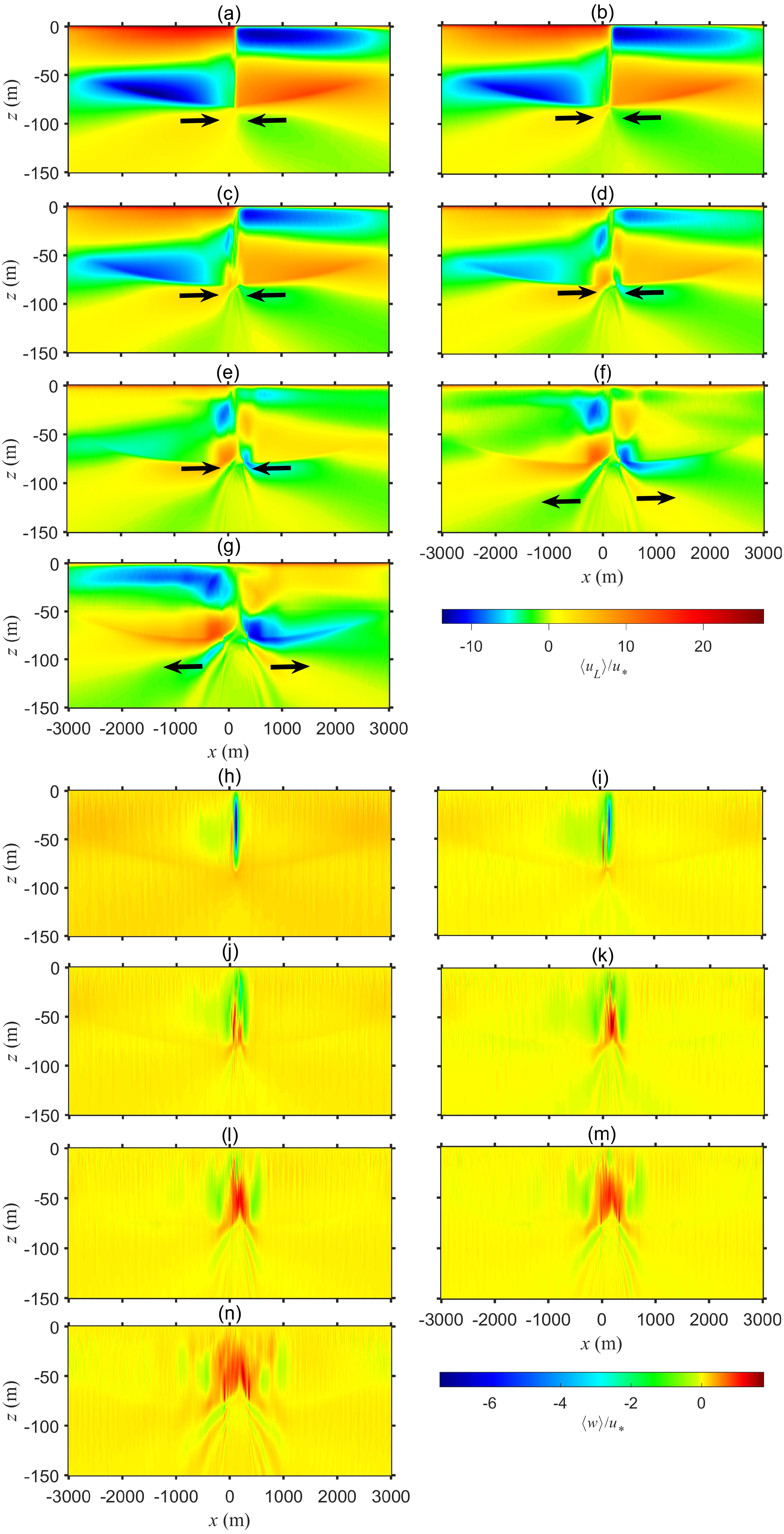
Filament frontolysis is a reverse process compared to filament frontogenesis (McWilliams, 2016). The direction of secondary circulations for filament frontogenesis is opposite to that for filament frontolysis (McWilliams, 2016). Hence, the conversion of filament frontogenesis to filament frontolysis is induced by a change in the direction of secondary circulations. In this section, we take
$ {u}_{*}/fh $ = 0.76 as an example to show a change in the direction of secondary circulations. Figure 13 shows the change in direction of secondary circulations with time. At the time stamp of the first arrest (tmnw = 3.37 h) in this simulation (Figs. 13a and h), the basic characteristics of secondary circulations are that the upper branches of the cross-filament currents flow toward the filament center, the lower branches of the cross-filament currents flow away from the filament center, and the main vertical current in the cold core range is a downwelling jet. The basic structure of secondary circulations at the time stamp of the first arrest (tmnw = 3.37 h) in this simulation (Figs. 13a and h) is consistent with the previous studies of McWilliams et al. (2015) and Sullivan and McWilliams (2018, 2019). Furthermore, it is worth noting that a clear upwelling jet appears near the left edge of the downwelling jet below z = −24 m (Fig. 13h). An upwelling jet near the left edge of the downwelling jet also appeared in the simulations of Sullivan and McWilliams (2018, 2019), but they did not discuss the upwelling current in their analysis. This upwelling jet is caused by the fact that the cross-filament currents below the upper mixed layer flow toward the left edge of the downwelling jet. This significant upwelling current essentially results from the unbalanced secondary circulations caused by the wind and wave fields in the interior of the upper mixed layer.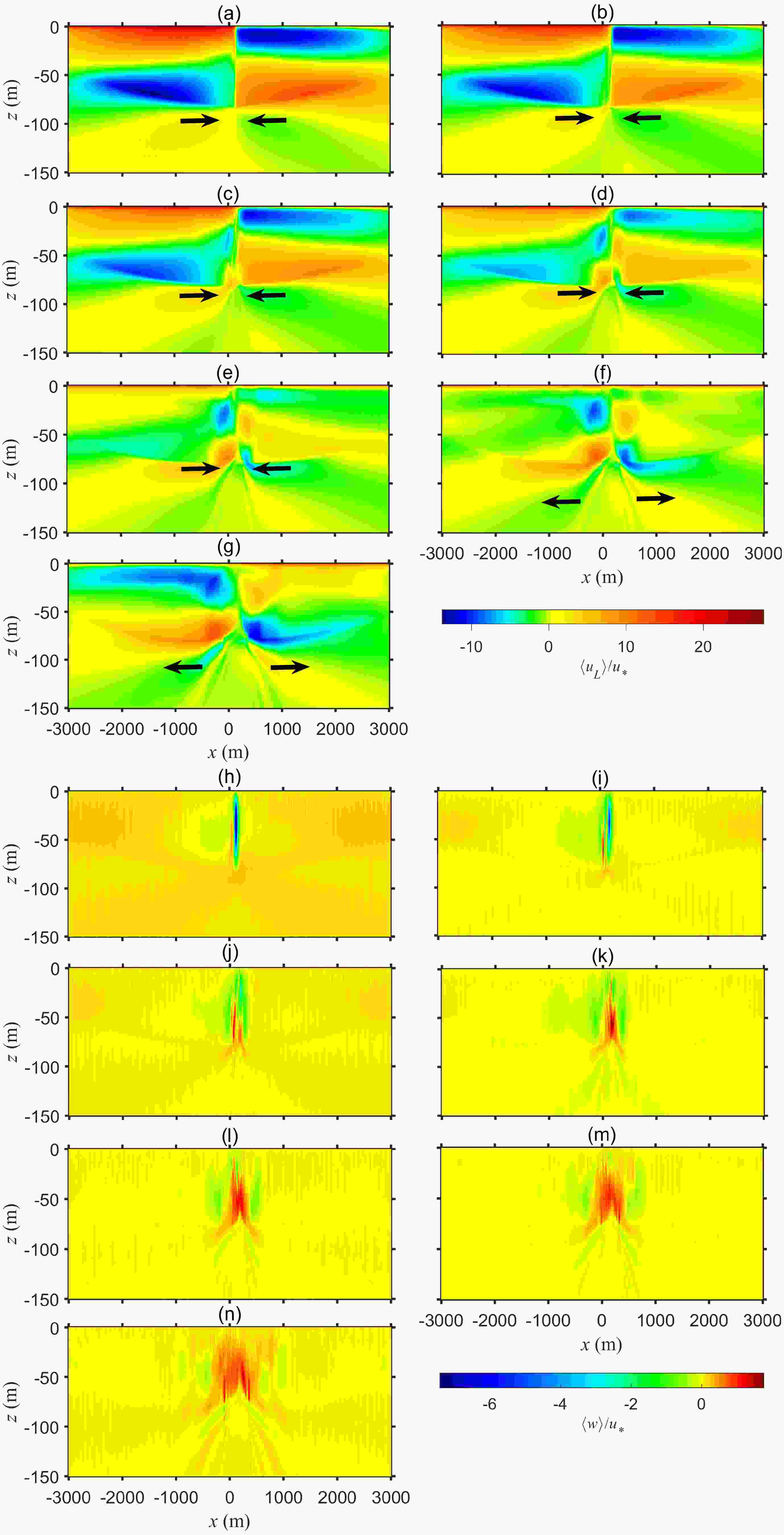
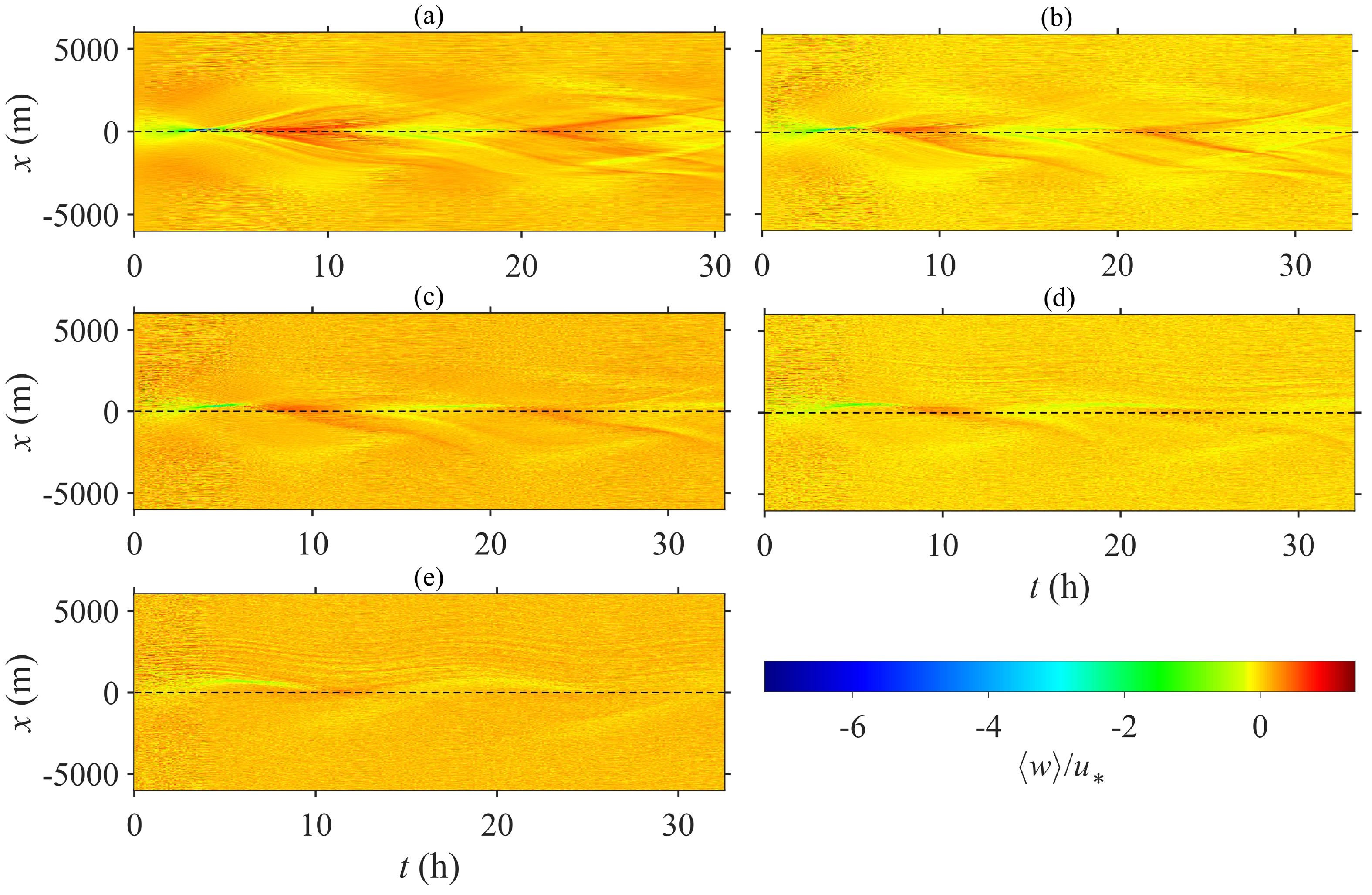
Figure 13. Conversion of the submesoscale current directions with time for
$ {u}_{*}/fh $ = 0.76. The normalized average flow fields of (a–g) the cross-filament currents$ \left\langle{{u}_{L}}\right\rangle/{u}_{*} $ and (h–n) the vertical currents$ \left\langle{w}\right\rangle/{u}_{*} $ at t = tmnw = 3.37 h and t = 3.91, 4.40, 4.96, 5.52, 6.26 and 7.18 h, respectively. The black arrows in (a–g) indicate the direction of the cross-filament currents below the upper mixed layer.Here, we illustrate a change process of the secondary circulation directions. As the time varies from t = tmnw = 3.37 h to t = 4.96 h, in the interior of the upper mixed layer the intensity of the secondary circulations—that is, the upper/lower branches of the cross-filament currents flow toward/away from the cold core, becomes weak, while below the upper mixed layer the intensity of the cross-filament currents flowing toward the cold core becomes strong (Figs. 13a–d). Thus, the downwelling jet weakens and the upwelling jet enhances (Figs. 13h–k) with the time changing from t = tmnw = 3.37 h to t = 4.96 h. Then, as the time changes from t = 4.96 h to = 7.18 h, the secondary circulations with the upper/lower branches of the cross-filament currents flowing toward/away from the cold core change into the secondary circulations with the upper/lower branches of the cross-filament currents flowing away from/toward the cold core (Figs. 13d–g). Meanwhile, the downwelling jet transforms into the upwelling jet (Figs. 13k–g). Hence, this result indicates a change in the direction of secondary circulations. In addition, below the upper mixed layer, the cross-filament currents flowing toward the cold core changes into that flowing away from the cold core (Figs. 13d–g), which will contribute to next conversion of the upwelling jet to the downwelling jet in the zone of the cold core (not shown). This result implies that if the filament frontogenesis does not induce the broken period of the cold filament within half of an inertial period (
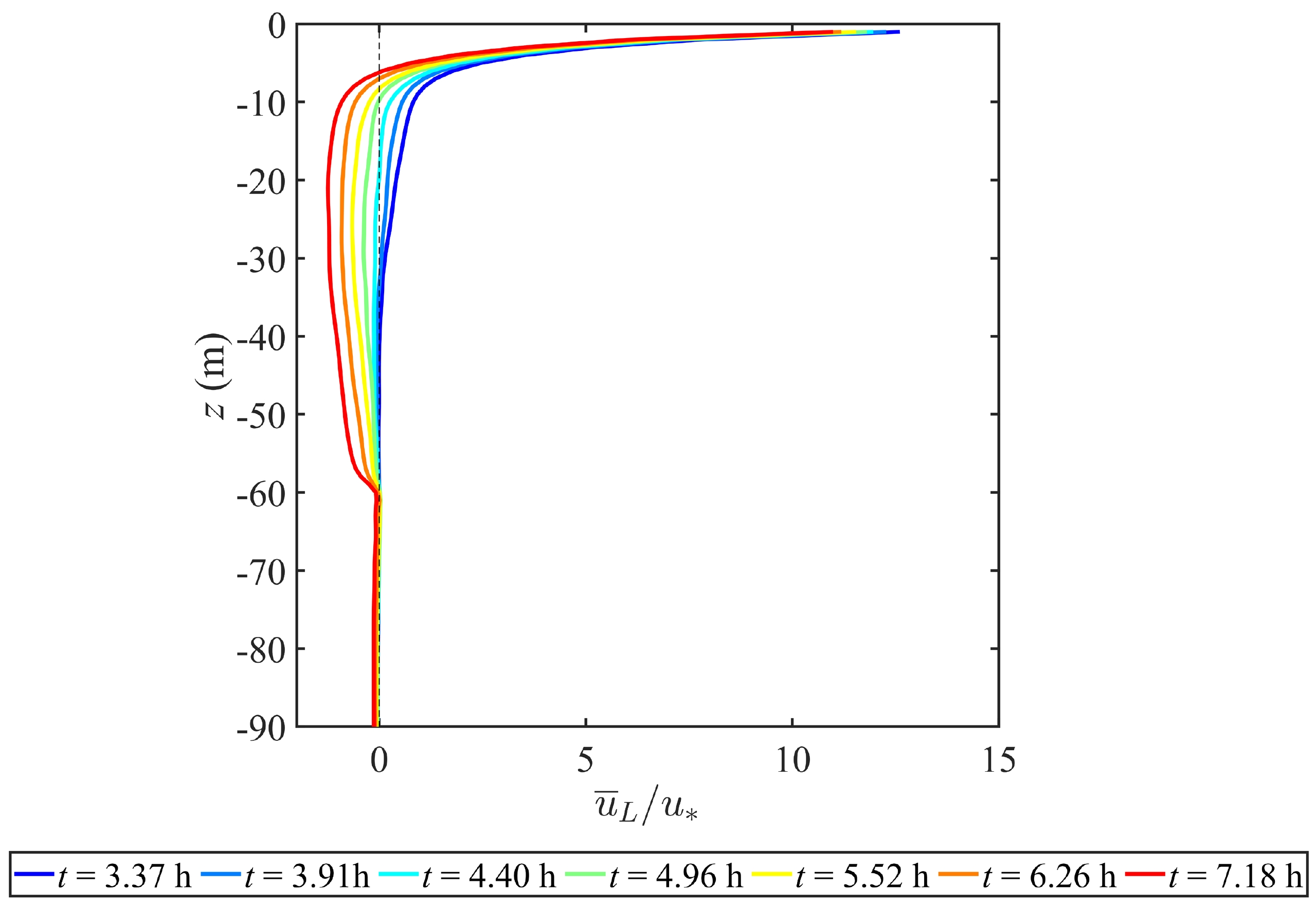
$ \pi /f $ ≈ 7 h) considered here, the filament frontolysis will happen in the next half of an inertial period (Figs. 9 and 11). Thus, the amplitude of the Coriolis parameter plays an important role in the frontogenetic trend of the cold filament.To further illustrate the effect of the cross-filament current created by the wind and wave fields on the asymmetries of secondary circulations and the relation between the directions of the cross-filament horizontal currents induced by the wind and wave fields and associated with the TTW relation, respectively, Fig. 14 shows the vertical profiles of the horizontal average (x–y plane average) cross-filament current
$ {\bar{u}}_{L}/{u}_{*} $ ($ {\bar{u}}_{L}=\bar{u}+{u}_{\mathrm{s}} $ is Lagrange velocity, in which an overbar represents the x–y plane average) created by the wind and wave fields in the remote fields of the cold filament at different time stamps corresponding to those in Fig. 13. At tmnw = 3.37 h, positive$ {\bar{u}}_{L}/{u}_{*} $ (Fig. 14) may strengthen (weaken) the positive (negative)$ \left\langle{{u}_{L}}\right\rangle/{u}_{*} $ branch of the left (right) secondary circulation above z = −30 m and has a weak effect on the left and right secondary circulations below z = −30 m (Fig. 13a). Then, with the time varying from tmnw = 3.37 h to t = 7.18 h, negative$ {\bar{u}}_{L}/{u}_{*} $ gradually appears and the amplitude and range of the negative$ {\bar{u}}_{L}/{u}_{*} $ increases, while the amplitude and range of the positive$ {\bar{u}}_{L}/{u}_{*} $ decreases, as shown in Fig. 14. Hence, the superposition of the$ {\bar{u}}_{L}/{u}_{*} $ (Fig. 14) and$ \left\langle{{u}_{L}}\right\rangle/{u}_{*} $ (Fig. 13) at different time stamps always breaks the symmetry of the left and right secondary circulations. A comparison of$ {\bar{u}}_{L}/{u}_{*} $ (Fig. 14) with$ \left\langle{{u}_{L}}\right\rangle/{u}_{*} $ (Fig. 13) suggests that, because of the presence of the cold filament, the change in the direction of the upper$ \left\langle{{u}_{L}}\right\rangle/{u}_{*} $ branch of the right secondary circulation with time induced by the Coriolis parameter (Fig. 13) is opposite to that of the$ {\bar{u}}_{L}/{u}_{*} $ created by the wind and wave fields in the remote fields of the cold filament (Fig. 14). This result indicates that the presence of the cold filament complicates the flow structures and the changes in the flow directions with time.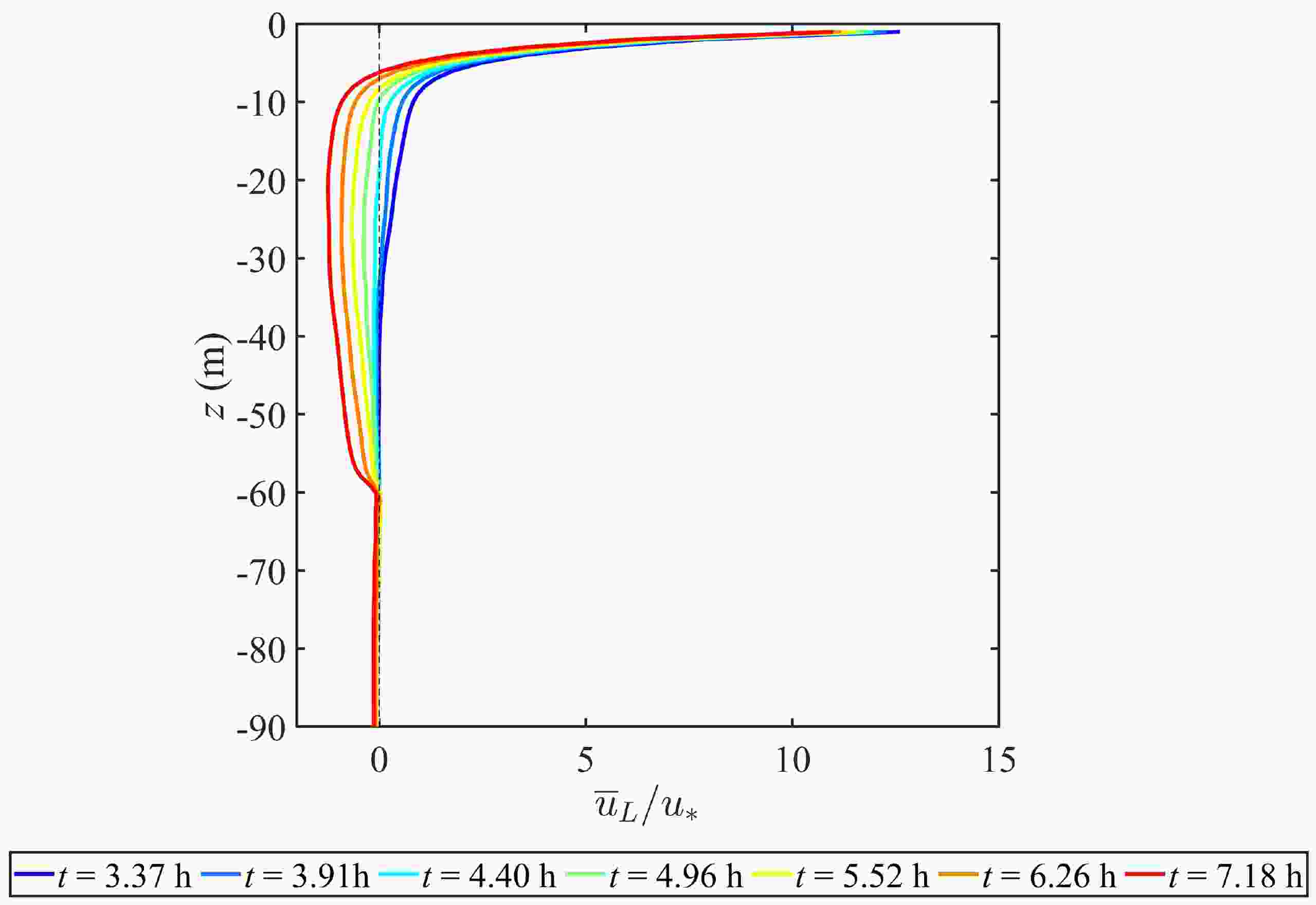
Figure 14. Vertical profiles of the normalized cross-filament currents
$ {\bar{u}}_{L}/{u}_{*} $ created by the wind and wave fields in the remote fields of the cold filament at t = tmnw = 3.37 h and t = 3.91, 4.40, 4.96, 5.52, 6.26 and 7.18 h, respectively, consistent with those in Fig. 13. -
A comparison of the variations in the ageostrophic secondary circulation
$ \left(\left\langle{{u}_{L}}\right\rangle,\left\langle{w}\right\rangle\right)/{u}_{*} $ (Figs. 9 and 11) and the temperature$ \left\langle{{T}_{\mathrm{s}\mathrm{o}}-{T}_{\mathrm{o}}}\right\rangle/\delta {T}_{\mathrm{o}} $ (Fig. 12) shows that, after the first period of filament frontogenesis and frontolysis, the effect of filament frontolysis significantly reduces with an enhancement of the wind and wave fields indicated by an increase of$ {u}_{*}/fh $ . Notably, as$ {u}_{*}/fh $ changes from$ {u}_{*}/fh $ = 1.37 to$ {u}_{*}/fh $ = 2.09, the downwelling current (the negative$ {\left\langle{w}\right\rangle}_{p}/{u}_{*} $ ) gradually plays a leading role in the vertical flow of the cold core zone (Fig. 2a and Fig. 11e) after the first period of the conversion of the secondary circulation directions (Figs. 2a, 9e and 11e), though the weak upwelling current (the positive$ {\left\langle{w}\right\rangle}_{p}/{u}_{*} $ ) still appears in the latter half of the secondary inertial period (Fig. 11e). Thus, the temperature$ \left\langle{{T}_{\mathrm{s}\mathrm{o}}-{T}_{\mathrm{o}}}\right\rangle/\delta {T}_{\mathrm{o}} $ in the cold core center has a significant rise after t = 23.1 h with$ {u}_{*}/fh $ varying from$ {u}_{*}/fh $ = 1.37 to$ {u}_{*}/fh $ = 2.09, as shown in Fig. 15. This result illustrates that, if the wind and wave fields are strong enough, the effect of filament frontolysis on the cold filament frontogenetic trend may be strongly inhibited by the wind and wave fields after the first period of filament frontogenesis and frontolysis.Furthermore, the filament frontogenesis and frontolysis (Figs. 9 and 11) may periodically break and restore the structure of the cold filament (Fig. 12), which should be an important reason for the lifetime of some submesoscale cold filament processes reaching a few days. The submesoscale currents and cold filament structures feature complex changes with variations in time and the strength of the wind and wave fields in this simulation, which implies that submesoscale processes need to be studied further to provide more information for parameterizing their effects on large-scale circulations. Bodner et al. (2023) advanced the parameterization of submesoscale processes to include the interactions with boundary layer turbulence through the turbulent convective velocity (
$ {w}_{*} $ ) and friction velocity ($ {u}_{*} $ ). Sullivan and McWilliams (2018, 2019) also showed that the submesoscale currents and frontogenesis levels of a cold filament are clearly different, when the direction of winds and waves is perpendicular and parallel to the filament axis. The results in this paper only illustrate the impact of the magnitude of the cross-filament wind and wave fields on the frontogenesis and frontolysis of a cold filament, and thus the effects of a change in the direction of the wind and wave fields on cold filament frontogenesis needs to be studied in the future.A density front with a one-side density (or buoyancy) gradient across its axis can be considered to be one half of a cold (dense) filament with two-side density (or buoyancy) gradients. The change in the direction of secondary circulations of a cold filament with time due to inertial oscillation should also be suitable for that of a density front in theory. The frontogenic process of a density front is beyond the scope of this article. We will study the frontogenic process of a density front in the future.
-
The differences in the cold filament frontogenetic trend as driven by different strengths of the cross-filament wind and wave fields were simulated by LES. An increase in the wind and wave fields may further break the symmetries of the submesoscale flow fields and suppress the level of cold filament frontogenesis. The periodic changes of the secondary circulation directions—that is, the conversion between convergence and divergence of the surface cross-filament currents with the downwelling and upwelling jets underneath the surface layer—are caused by the inertial oscillation. This leads to the filament frontogenesis and frontolysis periodically sharpening and smoothing the horizontal gradient of the submesoscale flow fields, respectively.
The lifecycle of cold filament frontogenesis may include multiple stages of filament frontogenesis and frontolysis due to the inertial oscillation induced by the Coriolis parameter in this simulation. The simple concept of cold filament frontogenesis only including the onset, arrest, decay, and broken periods (Sullivan and McWilliams, 2018, 2019) is not suitable for the simulation considered here. Hence, the basic stages of cold filament frontogenesis in Sullivan and McWilliams (2018, 2019) need to include the frontogenesis and frontolysis caused by inertial oscillation with a large value of the Coriolis parameter.
The present study shows that the amplitudes of the wind and wave fields and Coriolis parameter may modulate the magnitude, shape, structure and direction of the submesoscale flow fields. Future work on the different cold filament characteristics (e.g., the horizontal temperature gradient and the width of the cold core region) and Coriolis parameters is required to uncover the variations of the subumesoscale currents of cold filaments from various aspects. The study of submesocale processes can be used to explain the impact of these processes on the functioning of the oceanic system (McWilliams, 2021) and to parameterize their effects on oceanic circulation evolutions in large-scale oceanic circulation models (Capet et al., 2008c).
Acknowledgements. This research was supported by the National Natural Science Foundation of China (Grant Nos. 92158204, 41506001 and 42076019) and a Project supported by the Southern Marine Science and Engineering Guangdong Laboratory (Zhuhai) (Grant No. 311021005). The LES model was provided by the National Center for Atmospheric Research. All numerical calculations were carried out at the High Performance Computing Center (HPCC) of the South China Sea Institute of Oceanology, Chinese Academy of Sciences.
| Experiment | $ {u}_{*}/fh $ | $ {U}_{a} $ (m s−1) | $ {u}_{*} $ (10−2 m s−1) | $ {u}_{{\mathrm{os}}} $ (10−1 m s−1) | $ {\delta }_{s} $ (m) | $ {{\mathrm{La}}}_{{\mathrm{tur}}} $ | $ h $ (m) | $ f $ (10−4 s−1) |
| Exp.1 | 0.76 | 5 | 0.57 | 0.63 | 2.13 | 0.3 | 60 | 1.25 |
| Exp.2 | 1.07 | 7 | 0.80 | 0.88 | 4.15 | 0.3 | 60 | 1.25 |
| Exp.3 | 1.37 | 9 | 1.03 | 1.14 | 6.92 | 0.3 | 60 | 1.25 |
| Exp.4 | 1.71 | 11 | 1.28 | 1.42 | 10.32 | 0.3 | 60 | 1.25 |
| Exp.5 | 2.09 | 13 | 1.57 | 1.74 | 14.42 | 0.3 | 60 | 1.25 |


 AAS Website
 AAS WeChat