


 DownLoad:


-
Microphysics parameterization (MP) uncertainty remains a substantial source of numerical weather prediction (NWP) model error. One to two hydrometeor categories, demarcated by smaller cloud droplets and larger rain drops, can simulate spherical liquid particles with water density without much error. In contrast, parameterizations of ice particles in MP schemes continue to lag in sophistication relative to the complex geometrical spectra of observed ice habits. While ice crystal diagrams have documented observed habits for a given ambient temperature and ice supersaturation, the oscillatory nature of plates and columns with changes in temperature [as well as often-observed asymmetrical crystals and complex polycrystal structure (Bailey and Hallett, 2009)] preclude an exact, quantitative relationship linking ice crystal geometry to the ambient thermodynamic state. Aggregates of crystals may also form additional habits, with even more distinct habits if these ice particles rime (e.g., Magono and Lee, 1966; Heymsfield and Kajikawa, 1987; Pruppacher and Klett, 2010). Therefore, ice habits are inevitably oversimplified in NWP models, as it is impossible to parameterize every observed ice type with a few ice hydrometeor categories, such as the typically used cloud ice, snow/aggregates, graupel and/or hail.
The evolution of the particle size distribution (PSD) of a hydrometeor category in NWP models is typically modelled in either a bulk or spectral bin framework. Bulk MP schemes (BMPs) assume certain forms of hydrometeor PSDs containing a few free parameters (e.g., Lin et al., 1983; Ulbrich, 1983; Chen and Sun, 2002), while spectral bin MP schemes (SBMs) discretize the PSDs into spectral bins, generally predicting the evolution of either the PSDs themselves or moments in each bin (e.g., Hall, 1980; Reisin et al., 1996; Geresdi, 1998). SBMs’ discrete PSD bins allow the parameterization of particle attributes (e.g., axis ratio, density) with greater flexibility and precision than BMPs across the hydrometeor spectra, albeit at potentially higher computational costs. For more details, readers are referred to a comprehensive review of bulk and spectral bin schemes by Khain et al. (2015).
Despite many complex observed geometric modes of ice particles, MP schemes attempt to represent the ice spectra across a limited number of ice categories [e.g., cloud ice, snow, graupel, hail (Geresdi, 1998; Milbrandt and Yau, 2005a, b)]. BMPs include spherical (e.g., Ferrier, 1994; Morrison et al., 2009) and non-spherical crystal/snow (e.g., Cox, 1988; Hong et al., 2004) more consistent with observations (e.g., Mitchell et al., 1990). BMPs may contain constant (e.g., Ferrier, 1994) or predicted rimed ice density (e.g., Mansell et al., 2010). Further, the Predicted Particle Properties [P3 (Morrison and Milbrandt, 2015; Milbrandt et al., 2021)] and Ice-Spheroid Habit Model with Aspect-Ratio Evolution [ISHMAEL (Jensen et al., 2017)] BMPs remove distinct ice categories in favor of free-evolving ice particles in each category (although ISHMAEL contains a separate aggregate category for ice property preservation), reducing ad-hoc simulated ice conversions.
SBM PSD discretization allows for greater precision of ice particle and process parameterization compared to BMPs. Young (1974) and Takahashi (1976) partitioned ice crystal size bins into x- and z-dimensions, while separate ice crystal habits as hydrometeor categories (e.g., columns, dendrites) were also added to some SBMs (Khain and Sednev, 1996; Khain et al., 2004). The expansion from 33 to 43 bins within the Hebrew University Cloud Model (HUCM) SBM “full” version and improved graupel to hail conversion facilitated large rimed ice particles and reflectivities as simulated by a polarimetric radar simulator in deep convection (Ryzhkov et al., 2011). Still, increasing ice complexity using SBM hydrometeor representation does not always guarantee more accurate simulations relative to BMPs (e.g., Fan et al., 2017; Xue et al., 2017) because of a large number of uncertainties with the MP processes involved. While these papers and others (e.g., Kumjian et al., 2014; Shpund et al., 2019) demonstrate reasonable ability of SBMs to simulate deep convection, SBMs (and BMPs) require detailed assessment and understanding of hydrometeor evolution when applied to different types of convective storms.
Supercell microphysical processes are typically dominated by rain and rimed ice given the storm’s deep convective updraft (e.g., Kumjian and Ryzhkov, 2008). Simulated cloud water, cloud ice, and snow provide pathways to rain and rimed ice creation and growth [see Fig. 4 in Morrison et al. (2020)], highlighting their potential roles in particle evolution within supercell thunderstorms. Further, the limited three-dimensional idealized supercell simulation studies that exist using the Weather Research and Forecasting [WRF (Skamarock et al., 2008)] model coupled with HUCM “full” microphysics [HU-SBM (Khain and Lynn, 2009; Heikenfeld et al., 2019)] have mainly focused on model sensitivities (e.g., aerosol concentration) related to, rather than in-depth evaluations of, microphysical processes controlling SBM hydrometeor evolutions. In this study, we examine hydrometeor evolutions in idealized supercell simulations using the HU-SBM and two-moment NSSL and Thompson BMP schemes within the community WRF model. We investigate their underlying representations and MP processes primarily responsible for significant differences found in the simulations. Such a study can help clarify how each MP scheme simulates complex ice spectra and their impact on the liquid spectra, and provide guidance on improving the schemes’ representation and evolution of ice with a limited number of hydrometeor categories. Insights gained from analyzing idealized simulations can help guide future SBM/BMP improvement when applied to real cases by establishing a link between MP treatments and the expected results of storm simulation.
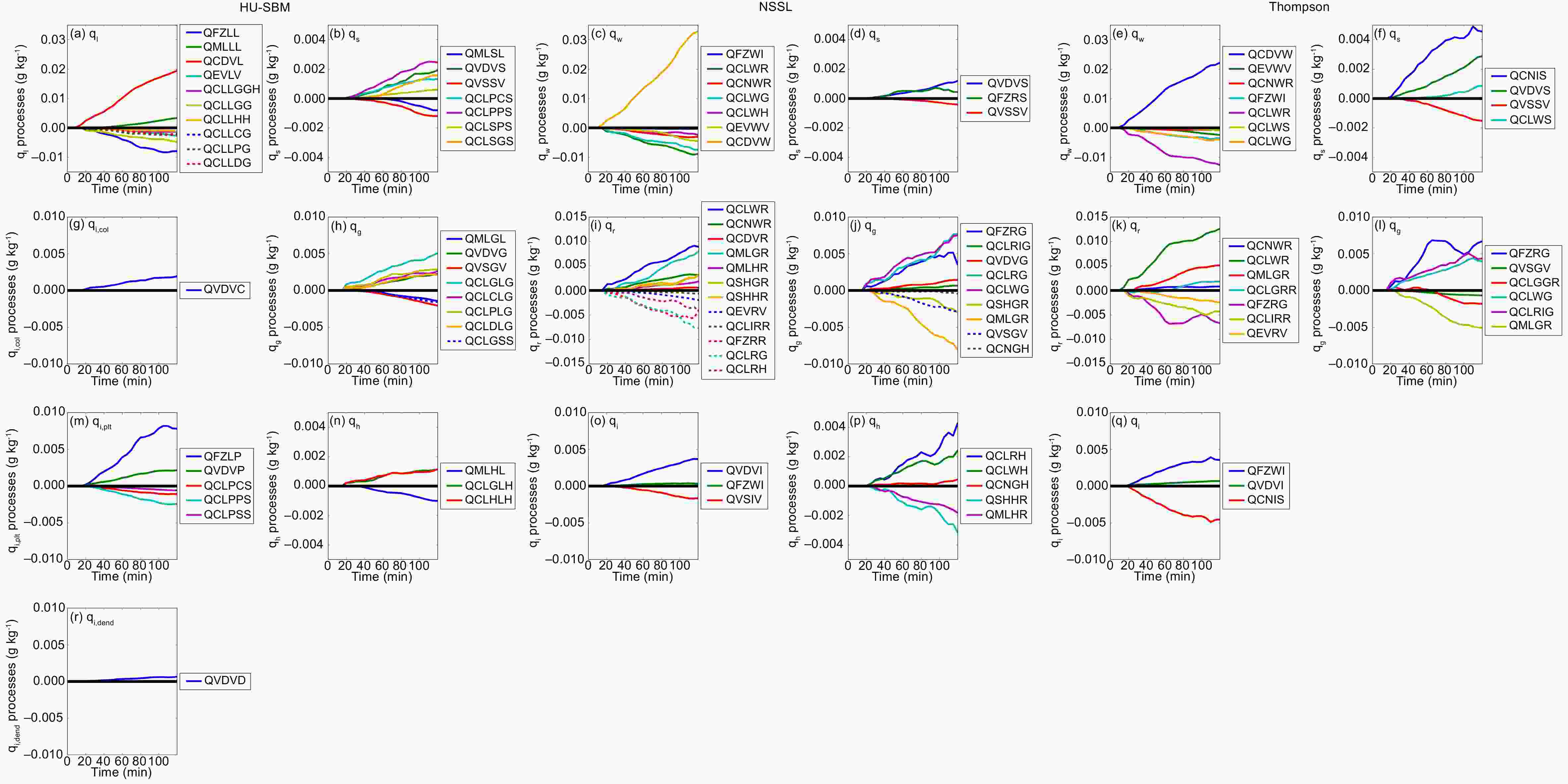
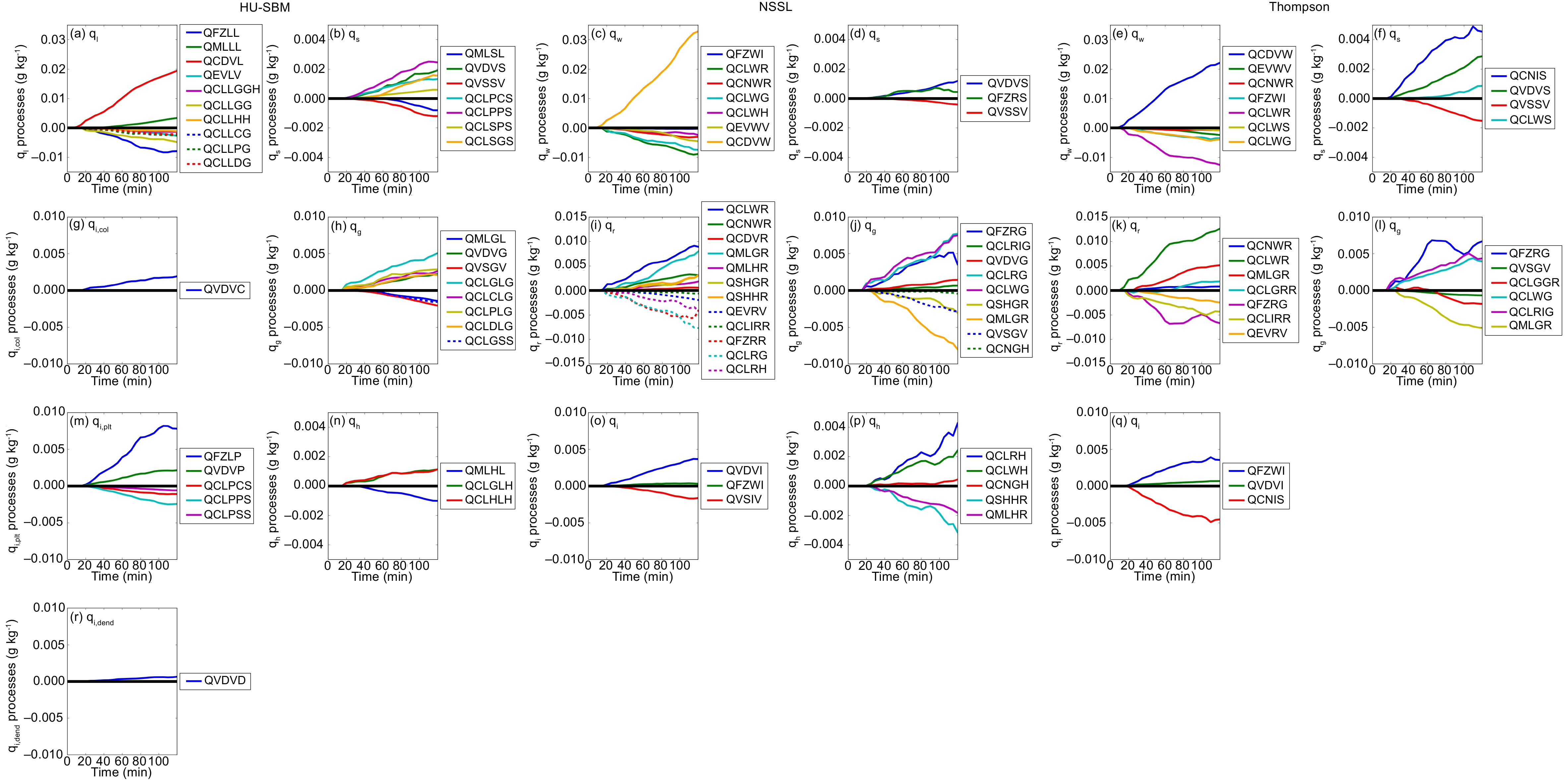
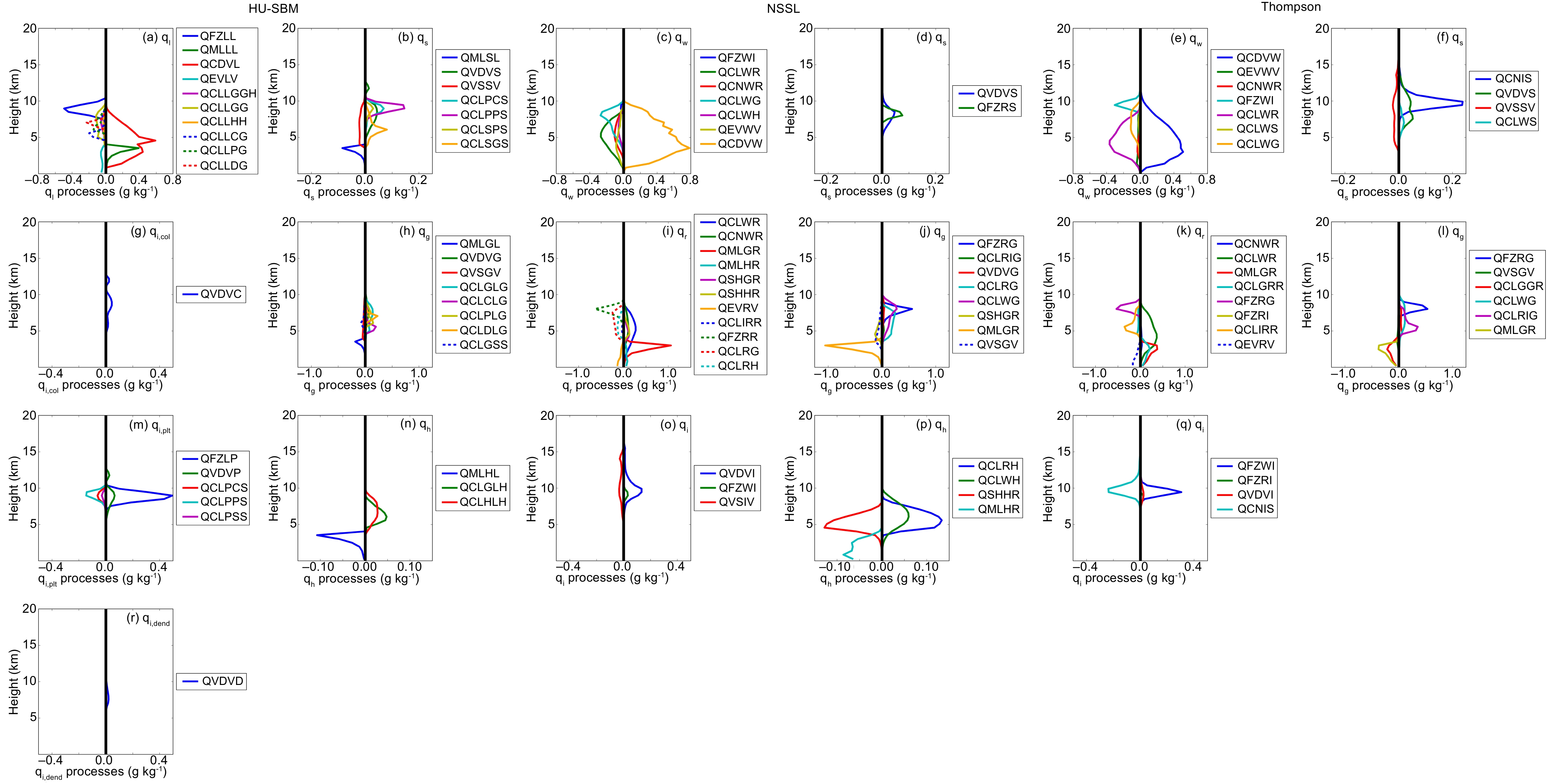
Figure 4. Domain-averaged 5-min accumulated mixing ratio process rates (units: g kg−1) for the (left two columns) HU-SBM, (middle two columns) NSSL, and (right two columns) Thompson microphysics schemes. Plot labels indicate the relevant hydrometeor.
The rest of this paper is organized as follows: section 2 details the simulation model setup; section 3 compares simulated precipitation and hydrometeor profiles to analyze hydrometeor behavior (e.g., potential relative biases) within the storm; section 4 investigates hydrometeor vertical flux profiles and their link to surface precipitation; and section 5 summarizes and further discusses dynamic and microphysical effects on precipitation in the spectral and bulk frameworks examined in this paper.
-
Idealized simulations of supercell thunderstorms are performed using the compressible, nonhydrostatic WRF model, version 3.7.1 (Skamarock et al., 2008). The model configuration is detailed in Table 1, and is similar to the idealized supercell simulations in Johnson et al. (2016, 2019). Storms are simulated for 2 h on a 200 km × 200 km grid with a 1 km horizontal spacing. The vertical grid extends to 20 km in height with an approximate 500 m grid spacing. The Weisman and Klemp (1982) thermodynamic sounding with a veering quarter-circle wind profile (clockwise shear of 5.23 × 10⁻³ s−1 up to 2.3 km, unidirectional shear of 5.69 × 10⁻³ s−1 above to 7 km) is employed for the atmospheric environment, resulting in a convective available potential energy (CAPE) of approximately 2163 J kg−1 and storm-relative helicity in the 0–3 km layer of approximately 180 m2 s−2. The storm is initiated using an ellipsoidal thermal bubble with a maximum potential temperature perturbation of 3 K. Radiation, land surface, cumulus, and planetary boundary layer parameterizations are turned off.
WRF model configuration Run time 120 min Δt 6 s Sound wave Δt 1 s Model output interval 10 min Horizontal domain 200 km × 200 km Model lid 20 km Δx 1 km Δy 1 km Δz ~500 m Time integration scheme Third order Runge–Kutta Horizontal momentum advection Fifth order Vertical momentum advection Third order Horizontal scalar advection Fifth order Vertical scalar advection Third order Upper level damping 5000 m below model top Rayleigh damping coefficient 0.003 Turbulence 3D 1.5-order turbulent kinetic energy closure Horizontal boundary conditions Open Table 1. WRF model input.
-
As mentioned earlier, three MP schemes with varying degrees of complexity in representing hydrometeors, as available in WRF v3.7.1, are used in the supercell simulations. They are, respectively, the HUCM “full” SBM (Khain and Sednev, 1996; Khain et al., 2004), the fully two-moment NSSL (Mansell et al., 2010), and the partially two-moment Thompson (Thompson et al., 2008) BMP schemes.
The HU-SBM “full” scheme prognoses the PSDs of liquid (one category spanning all drop sizes), three ice crystals (plates, columns, dendrites), (snow) aggregates, graupel, and hail, which are discretized into 33 mass-doubling bins ranging from 3.35 × 10⁻¹¹ to 1.44 × 10⁻¹ g. There are no processes in the HU-SBM “full” scheme that convert ice crystal habit to other habits after nucleation (in which the ice crystal destination is determined by ambient temperature). An alternative “fast” (in contrast to “full”) version of HU-SBM available in WRF prognoses the PSDs of one liquid and fewer ice categories, including ice crystals/aggregates, and graupel/hail, that are discretized into 33 or 43 bins. Studies have shown that the HU-SBM “fast” version has skill simulating deep convection (e.g., Khain et al., 2016; Shpund et al., 2019). In this study, we choose to evaluate the HU-SBM “full” version because of its inclusion of more ice categories (six versus two), which we believe are important for supercell storms. The use of 33 bins with smaller maximum diameters than the available 43 bins in the “fast” version does impose some limitation; therefore, results related to the maximum bin sizes do not necessarily carry over to the “fast” version. Hereafter, HU-SBM with no qualifier refers to the “full” version.
The NSSL BMP prognoses the mass mixing ratio qx and total number concentration NTx (x refers to species) of cloud water, rain, cloud ice, snow, graupel, and hail, and additionally the particle volume of graupel and hail, which can be used to predict the bulk density. The Thompson scheme prognoses the qx of cloud water, rain, cloud ice, snow, and graupel, and the NTx of cloud ice and rain. Among many available BMPs, the NSSL scheme is one of the most sophisticated two-moment BMPs and has been shown to outperform other BMPs in supercell simulations (Johnson et al., 2016, 2019), while the Thompson scheme is employed in the U.S. operational High-Resolution Rapid Refresh forecasting system (Benjamin et al., 2016) and has generally good performance for precipitation forecasting.
It is important to note that the hydrometeors in each MP scheme may contain different assumptions of PSDs and particle properties. Liquid, plates, graupel, and hail in the HU-SBM contain constant bulk densities of 1000, 900, 400, and 900 kg m−3, respectively, across their discretized mass bins, while column, dendrite, and snow bulk densities decrease at larger mass. Rain, graupel and hail in the NSSL scheme assume gamma PSDs (e.g., Ulbrich, 1983) with shape parameters of α = 0, 0, and 1, respectively. Cloud water, cloud ice, and snow have mass-dependent (rather than the commonly utilized diameter-dependent) gamma distributions with shape parameters of α = 0, 0, and −0.8 (Zrnic et al., 1993) respectively. Cloud water, cloud ice, rain, and snow have bulk densities of 1000, 900, 1000, and 100 kg m−3 respectively. Graupel and hail bulk densities are predicted via their bulk prognosed volumes. The Thompson scheme assumes an exponential PSD (gamma PSD with a shape parameter of α = 0) for cloud ice, rain, and graupel, and a gamma PSD (α = 12) for cloud water. Snow in the scheme follows a linear combination of exponential and gamma PSDs (Field et al., 2005; Thompson et al., 2008). Cloud water, cloud ice, rain and graupel have bulk densities of 1000, 890, 1000 and 500 kg m−3, respectively, while snow density decreases with increasing diameter (similar to HU-SBM snow).
-
The supercells simulated using the three schemes are first examined in terms of the simulated horizontal reflectivity ZH through the updraft (Fig. 1). ZH is calculated using the Center for Analysis and Prediction of Storms Polarimetric Radar data Simulator (e.g., Jung et al., 2008; Dawson et al., 2014; Johnson et al., 2016), which utilizes the T-matrix method (Waterman, 1969; Vivekanandan et al., 1991) to calculate scattering amplitudes as a function of the particle diameter and water fraction. The particle diameter is calculated assuming a spherical shape using the mass bins of hydrometeors in HU-SBM. The qx and NTx in the two-moment bulk schemes are utilized to diagnose hydrometeor PSDs, while the water fraction is diagnosed following Jung et al. (2008). For the HU-SBM scheme, the wet snow diameter is recalculated based on the mixed-phase hydrometeors’ new density, taking into account the shrinking of the horizontal dimension of snow with progressive melting as in Jung et al. (2008). Given the ice crystal complexity of HU-SBM, ice crystals are now included in the simulator for the scheme and are assumed to melt when the ambient temperature exceeds 0°C. Columns, plates, and dendrites are assumed to have aspect ratios of observed solid columns (L/d ≤ 2, L for crystal length and d for crystal thickness), solid thick plates, and dendrites, respectively (Matrosov et al., 1996). Oblate (i.e., plates and dendrites) crystal orientation is assumed to follow a two-dimensional axisymmetric Gaussian distribution with a mean canting angle of 0° and standard deviation of 10°, while prolates (i.e., columns) follow a blend of fully chaotic and horizontal random orientation (Ryzhkov et al., 2011). For other hydrometeor orientation assumptions, we refer the reader to Johnson et al. (2016).
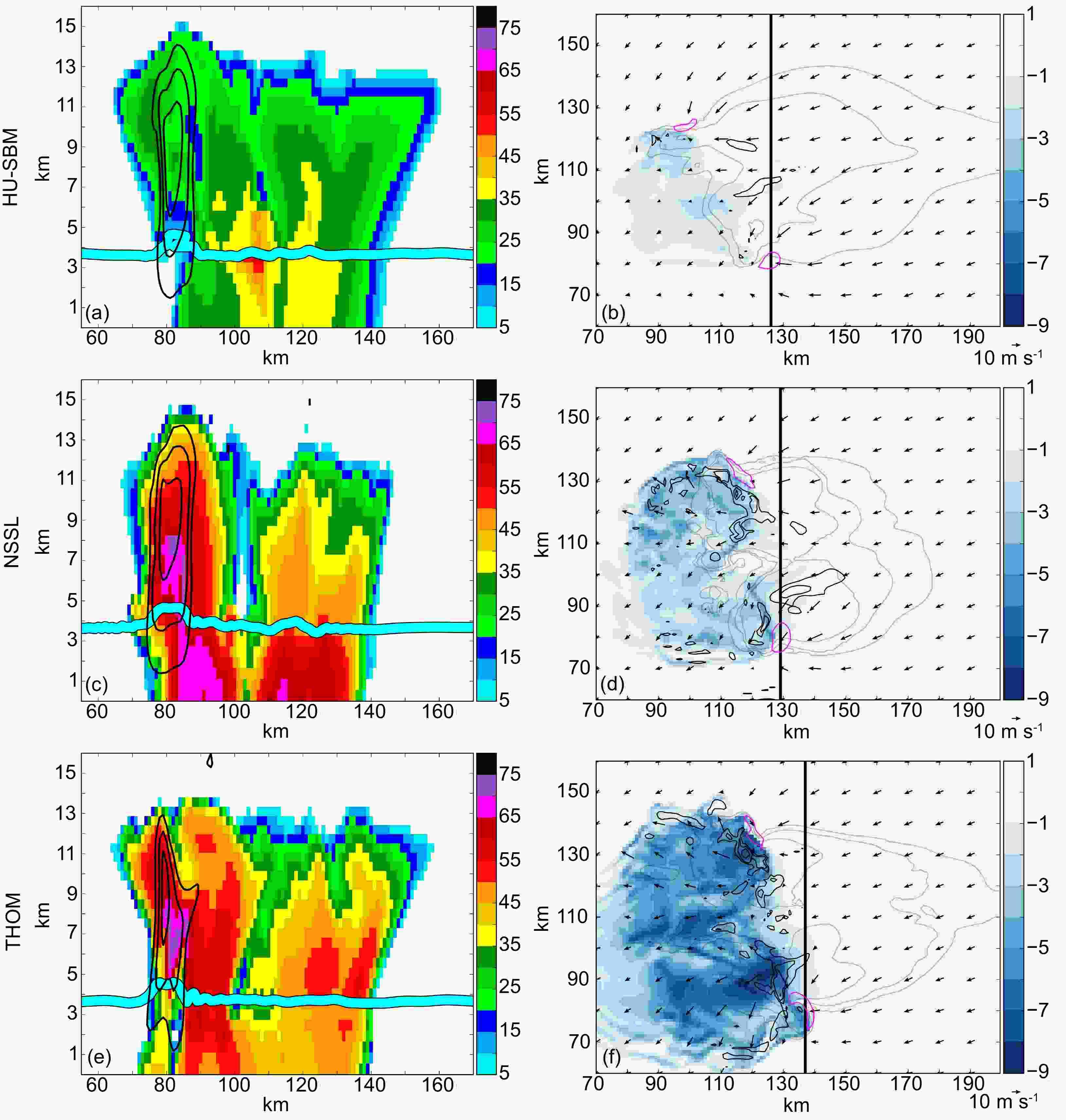
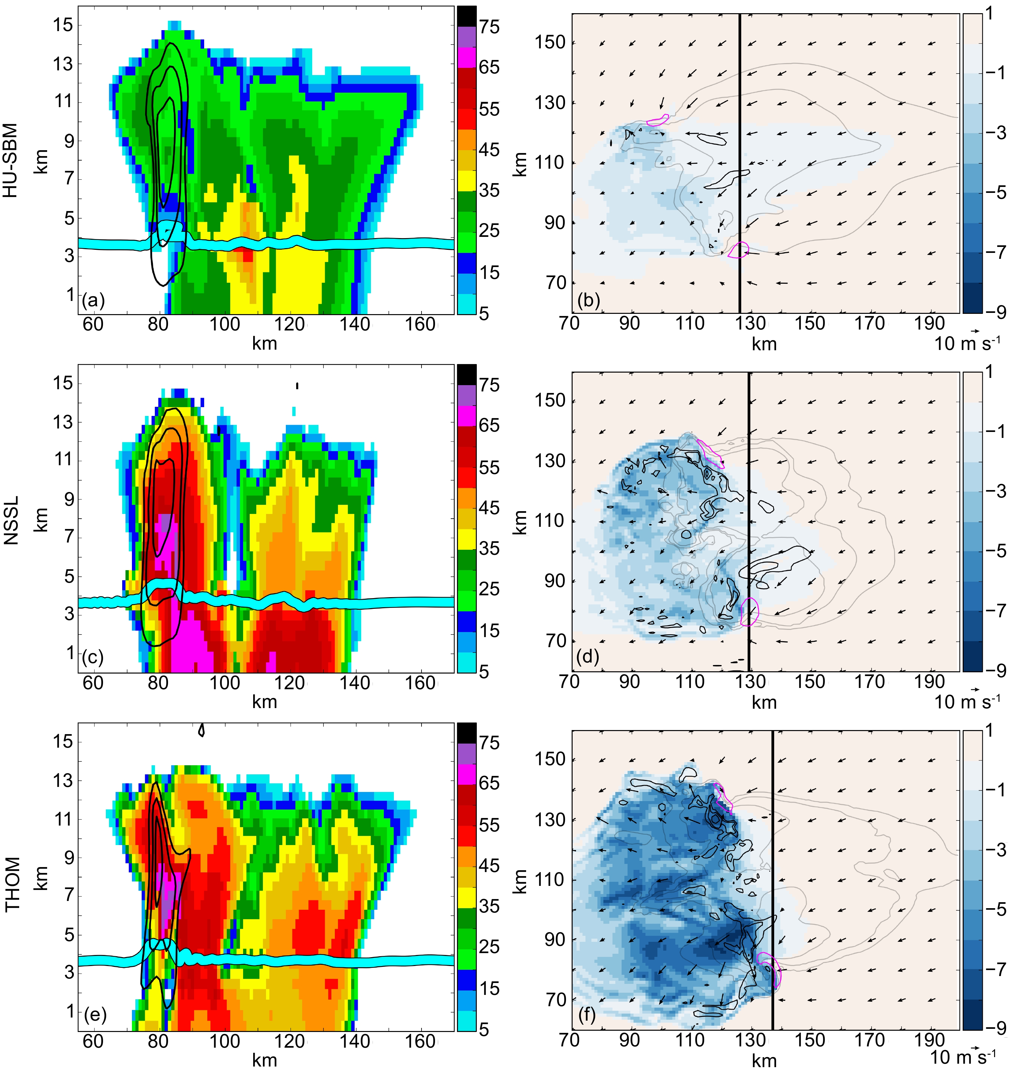
Figure 1. Horizontal reflectivity [ZH (units: dBZ); left column] through each storm’s updraft and potential temperature perturbations Ɵ' (units: K; right column) near z = ~280 m for the (a, b) HU-SBM, (c, d) NSSL, and (e, f) Thompson microphysics schemes at t = 100 min. Blue lines in vertical cross sections denote the 0°C isotherm, while black contours are vertical velocity, which start at 10 m s−1 with a 15 m s−1 interval. Reflectivity contours (grey) are shown in Ɵ' subplots for 15, 30, and 45 dBZ, and the wind field is represented by vectors. Updraft contours at z = ~2 km are shown as magenta contours for w = 10 m s−1, while downdraft contours at z = ~2 km are shown as black contours for w = −10, −5, and −2 m s−1 in Ɵ' subplots. Vertical black lines in Ɵ' plots denote where vertical cross sections are taken.
The storms simulated with the NSSL and Thompson BMPs have noticeably larger reflectivities than those of HU-SBM through their updraft cores at a mature supercell stage (t = 100 min; Fig. 1a, c and e), consistent with the reflectivity calculated in the microphysics schemes using the Rayleigh approximation. As the reflectivity in these simulations is primarily dictated by rain, graupel, and hail (as expected in a deep, convective storm), further hydrometeor analysis will help clarify which parameterizations/processes (e.g., wet growth, fall speed) are primarily responsible for the low reflectivity when HU-SBM is employed compared to the two bulk schemes. We also note that HU-SBM’s (snow) aggregate contribution to reflectivity is larger and more widespread near and below the melting level compared to those in simulations using the two bulk schemes. Because of their small sizes, the contribution of HU-SBM ice crystals to reflectivity is generally small. Differences are also seen in the cold pool structures of the MP storm simulations (Figs. 1b, d and f). The cold pool intensity reflects the downdraft intensity, water loading, and evaporative/melting cooling. Later analyses on the microphysical process rates will reveal differences in evaporative cooling among the simulations. The Thompson simulation, which has the strongest downdrafts, produces the strongest cold pool (Fig. 1f). HU-SBM downdrafts are weaker than those in the NSSL simulation, leading to a much weaker cold pool (Figs. 1b and d). Stronger downdrafts may influence precipitation by transporting more mass to lower levels in addition to hydrometeor sedimentation.
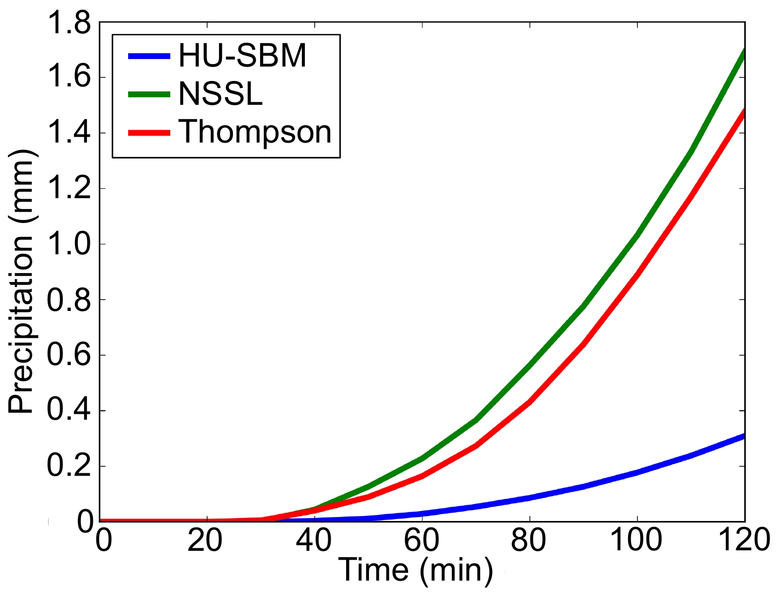
One striking difference between the three simulations differing in microphysics only is the large discrepancy of domain-averaged accumulated precipitation, with the NSSL and Thompson simulations producing similar precipitation amounts that are approximately five times that (~1.45–1.7 mm) of the HU-SBM simulation (~0.3 mm) by the end of the two-hour runs (Fig. 2). We note here that precipitation in the HU-SBM simulation might be delayed, as its domain-averaged accumulated precipitation near t = 200 min is similar to those of the bulk simulations near t = 120 min. HU-SBM precipitation is still smaller than those of the two bulk simulations when extended to 5 h (not shown). We also note that the HU-SBM “fast” version with 43 bins simulates precipitation amounts similar to those in the NSSL and Thompson simulations; however, it is outside the scope of this paper to determine the causes of the simulation differences between the “fast” and “full” versions. The comparatively low amount of precipitation simulated using the HUCM “full” MP has been previously noted in idealized supercell simulations. Khain and Lynn (2009) speculated that the much stronger updrafts (and possibly larger autoconversion rate) in the Thompson simulation compared to those in HU-SBM helped contribute to its larger amount of precipitation. Our HU-SBM simulation contains an updraft speed comparable to those of the NSSL and Thompson simulations (Fig. 1). Falk et al. (2019) noted the HUCM “full” MP simulated more precipitation when using faster snow, graupel, and hail bulk fall speeds applied to its bins, but still less than the amount produced by the bulk simulations. The influence of microphysics was not investigated further. Therefore, an investigation into rain and ice hydrometeor mass and related processes, and vertical hydrometeor fluxes, are needed to understand the key causes of the precipitation differences between the HU-SBM and bulk simulations.
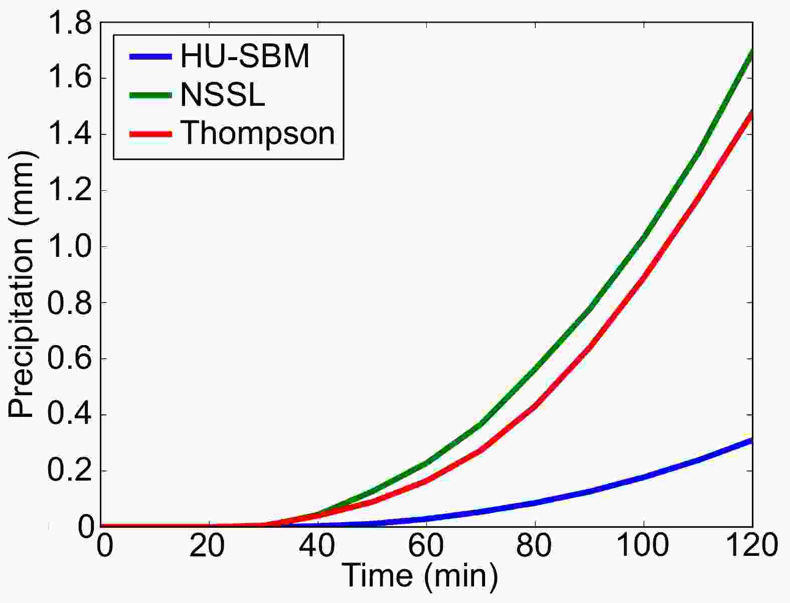
Figure 2. Domain-averaged accumulated precipitation (units: mm) over the duration of the model run for the HU-SBM, NSSL, and Thompson microphysics schemes.
-
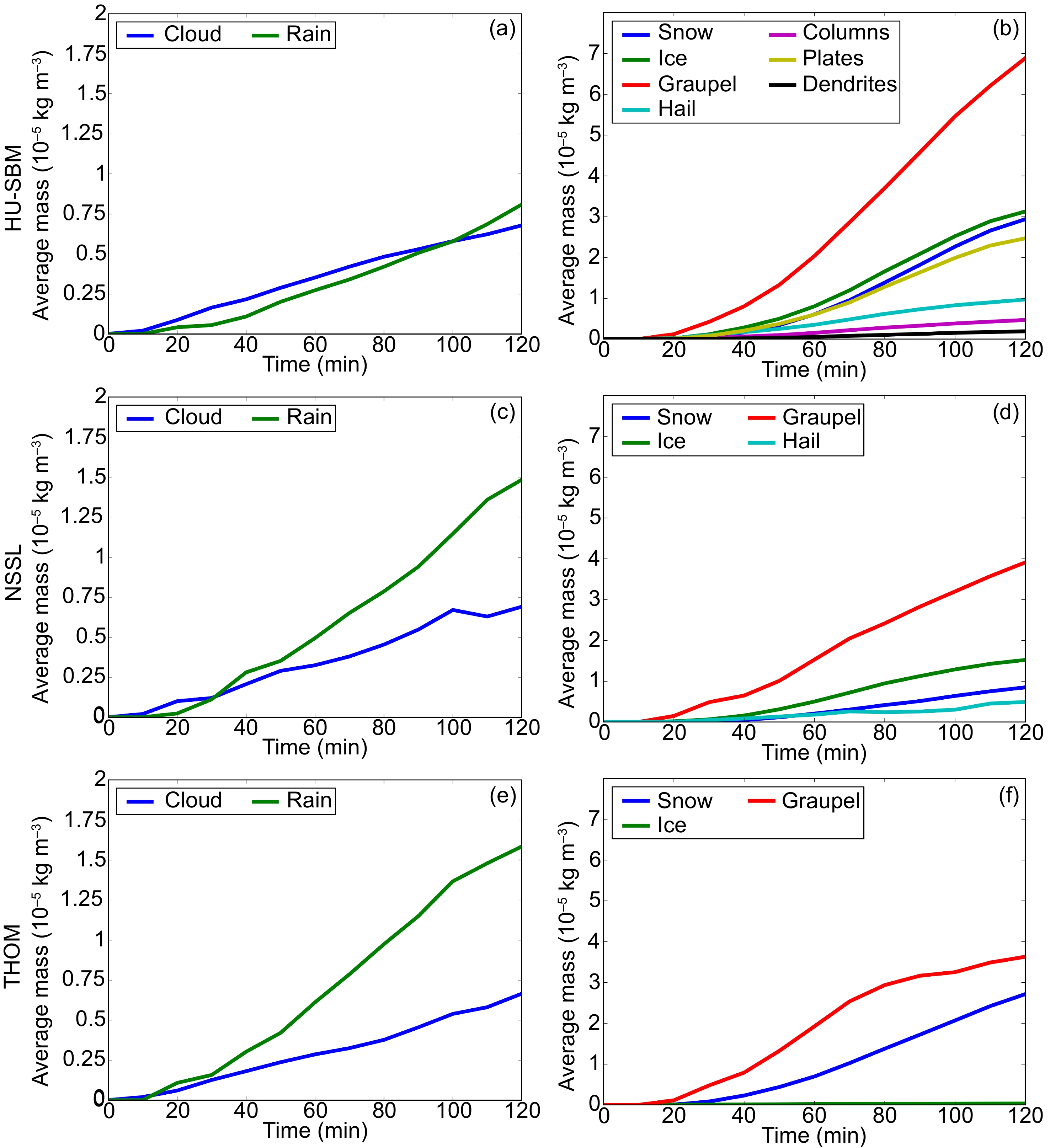
As MP-simulated hydrometeors directly contribute to the amount of available mass to sediment to the surface, it is logical to investigate the temporal evolution of each simulation’s domain-averaged mass (Fig. 3). Figure 4 shows the time series of domain-averaged 5-min accumulated microphysics rates for different species. While there is no traditional cloud water category in HU-SBM because all liquid is contained in its liquid hydrometeor category, HU-SBM does output “cloud water” mass corresponding to liquid bins with a maximum diameter of 0.16 mm, above which it is considered “rain”. We have included both liquid mass partitions to facilitate comparisons with the two bulk cloud water and rain masses. However, these partitions are not included when examining process rates, as processes rarely utilize this delimiter.
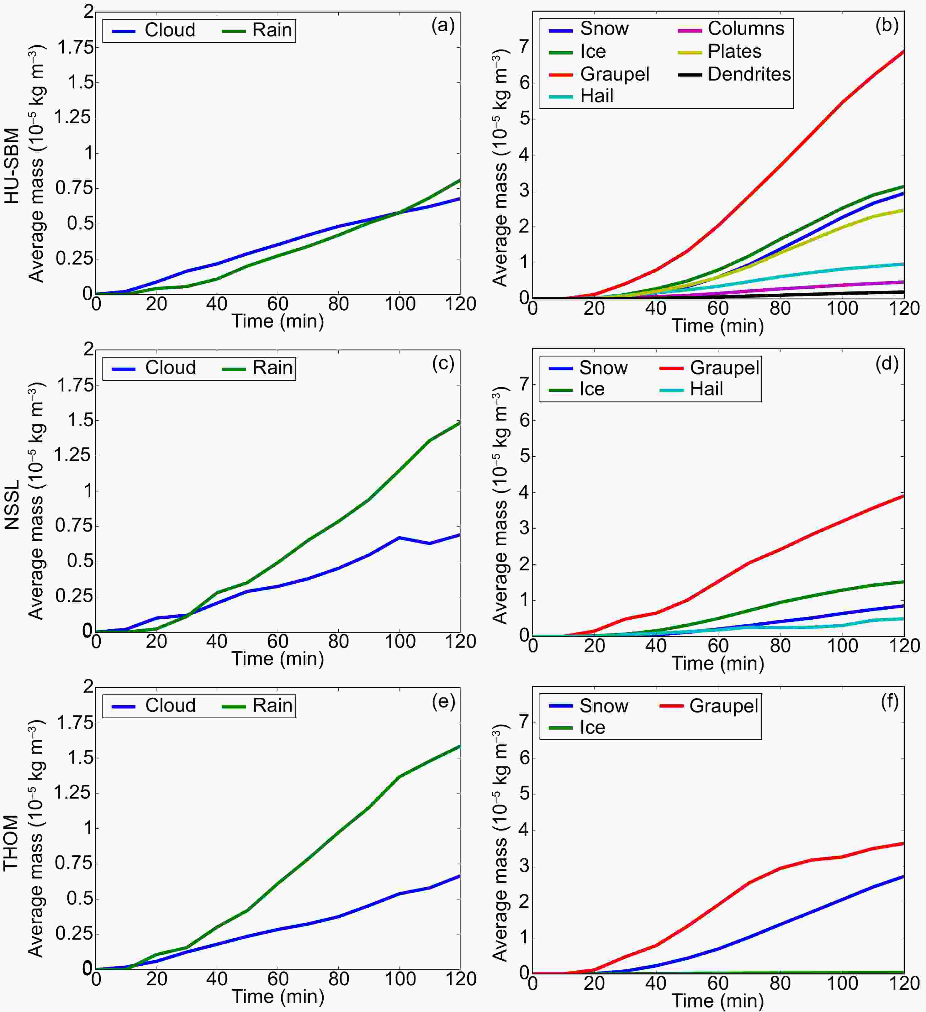
Figure 3. Time series of domain-averaged mass (units: kg m−3) for (a, c, e) liquid and (b, d, f) ice hydrometeors for the (a, b) HU-SBM, (c, d) NSSL, and (e, f) Thompson microphysics schemes over the duration of the model run.
The naming of the process rates in Fig. 4 uses the following conventions: Q refers to the mixing ratio; the next two letters describe the microphysical process [FZ—freezing, ML—melting, CD—condensation, EV—evaporation, CL—collection (or collision in HU-SBM), VD—vapor deposition, VS—vapor sublimation, CN—conversion, and SH—shedding]; and the next two letters generally denote the sink and source mass categories, respectively (V—vapor, L—liquid, W—cloud water, R—rain, C—column, P—plate, D—dendrite, I—cloud ice, S—snow, G—graupel, and H—hail). HU-SBM collisions have the next two letters after CL as the input colliding particles, while the final (or final two) letter(s) are source mass categories from the collision. For liquid, QFZLL and QMLLL denote total freezing and melting liquid mass changes, respectively. In the NSSL simulation, QFZRR and QCLIRR similarly denote total freezing, and rain and ice freezing rain mass changes, respectively. QCLRIG denotes rain and ice freezing to graupel. In the Thompson simulation, QCLGRR denotes possible rain source/sinks for graupel collecting rain, or vice versa depending on the ambient temperature. QCLGGR is similar to QCLGRR, but for graupel mass. Finally, QCLRIG denotes rain and ice freezing to graupel, while QCLIRR represents the rainwater sink from rain and ice freezing.
The cloud water mass is similar in the three simulations over the model run (Figs. 3a, c, e). Condensation of liquid/cloud water dominates the sources for these categories (Figs. 4a, c and e). Cloud water itself likely does not contribute much to accumulated precipitation, but subsequent evolution (e.g., rain collection, riming) can modify it. The rainwater mass is much larger in the bulk simulations, being close to 1.5 × 10⁻⁵ kg m−3 by the end of the model runs, compared to the HU-SBM rainwater mass exceeding 0.75 × 10⁻⁵ kg m−3. A reduction in rainwater mass relative to those in the two bulk simulations is consistent with the smaller precipitation in the HU-SBM simulation. The largest liquid sinks in HU-SBM are either freezing, graupel riming, or collisions with ice particles to form graupel. The largest rain sources in both the NSSL (Fig. 4i) and Thompson (Fig. 4k) simulations are rain collecting cloud water and melting graupel, and are larger than the HU-SBM liquid sources (presumably not including cloud water condensation; Fig. 4a). The Thompson simulation produces more rain than the NSSL simulation over the model run, in agreement with the NSSL rain sinks (e.g., wet growth, freezing) exceeding those in Thompson rain (e.g., freezing, cloud ice-rain freezing). Still, the NSSL simulation precipitates more mass to the surface, which motivates our later examination of vertical hydrometeor and flux profiles.
The amount of cloud ice mass in HU-SBM, which is the sum of its column, plate, and dendrite mass, exceeds the NSSL- and Thompson-simulated cloud ice mass (Figs. 3b, d, f). This is entirely due to the large amount of liquid freezing to plates in HU-SBM (Figs. 4g, m and r). The NSSL and Thompson schemes also freeze liquid (i.e., cloud water) into cloud ice (Figs. 4o and q), although not as much as HU-SBM. The small amount of cloud ice in the Thompson simulation is consistent with prior studies: the scheme is known to aggressively convert cloud ice to snow (e.g., Van Weverberg et al., 2013) as per the scheme’s design (Fig. 4q). The column mass exceeds the dendrite mass in HU-SBM, likely because of its larger nucleation temperature range. The snow mass is similar between the HU-SBM and Thompson simulations, which exceed that in the NSSL simulation. Snow aggregates in HU-SBM form by particle collisions; the large amount of HU-SBM plates provides a collisional source for aggregates, whether with themselves, other cloud ice particles, or aggregates (Fig. 4b). The primary source of NSSL snow is freezing rain (Fig. 4d), which provides a larger source for graupel than snow.
The rimed ice mass is typically largest in HU-SBM, as its simulated graupel mass is nearly two times larger than those of NSSL and Thompson by the end of the model run (HU-SBM graupel of ~7 × 10⁻⁵ kg m−3 versus NSSL and Thompson graupel of ~3.5–4 × 10⁻⁵ kg m−3; Figs. 3b, d, f). Much of HU-SBM’s graupel comes from cloud ice freezing with liquid to graupel, and primarily grows by riming (Fig. 4h). The largest graupel creation source in bulk simulations is freezing rain (although rain and ice freezing to graupel is prominent in the Thompson simulation; Figs. 4j and l), and grow by wet growth. The bulk simulations have similar graupel mass source magnitudes but larger graupel sinks (i.e., melting) at the end of the model run compared to HU-SBM, explaining its larger graupel mass. This also implies graupel production and wet growth is likely not a major deficit of HU-SBM. Thompson’s graupel mass is typically larger than NSSL’s over the model run, except at the end. While this might be related to the large amount of rain freezing in the Thompson simulation and larger NSSL graupel sinks, Fig. 4 does not include the graupel sinks from sedimentation. HU-SBM’s hail mass is larger than that of NSSL at the end of the model run (HU-SBM hail of ~1 × 10⁻⁵ kg m−3 versus NSSL hail of ~0.5 × 10⁻⁵ kg m−3). NSSL’s hail has larger sources (wet growth; Fig. 4p) than HU-SBM’s hail (graupel and liquid freezing to hail, wet growth; Fig. 4n), but also larger sinks (melting and shedding versus HU-SBM’s melting). More HU-SBM rimed ice does not lead to a larger rainwater mass field (i.e., melting) or accumulated precipitation. Again, we note that downdrafts are typically stronger in the bulk simulations than in HU-SBM. This motivates a further investigation into the vertical distributions of hydrometeors, hydrometeor fluxes, and bin/bulk PSD assumptions to determine their effects on precipitation, the results of which will be presented later.
-
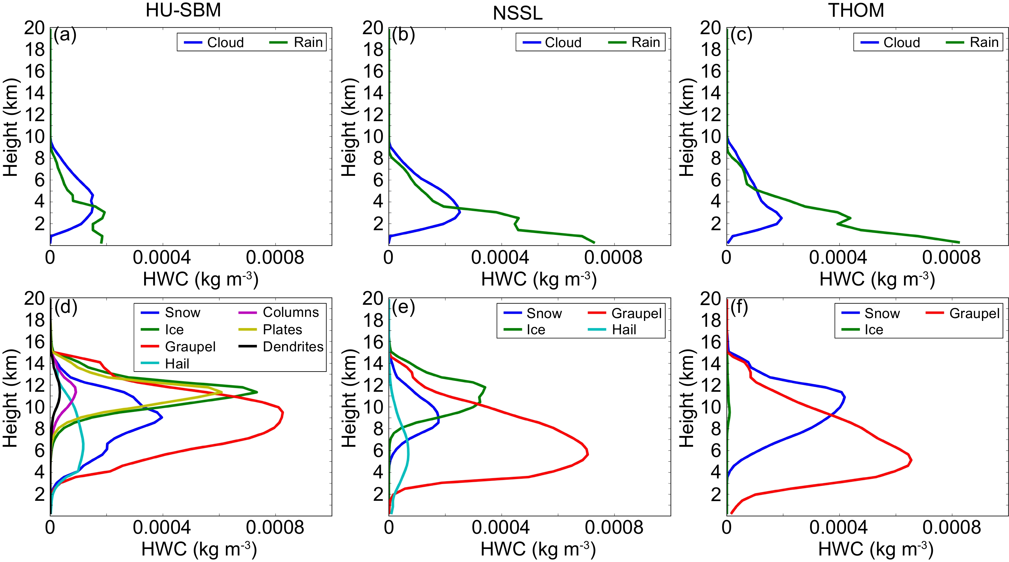
Vertical profiles of hydrometeor water content (HWC) are taken at a mature supercell stage (t = 100 min; Fig. 1) to show their vertical distributions at this time (Fig. 5). At each height level, the horizontal average of water content is calculated over the domain where the condensate mixing ratio exceeds 0.01 g kg−1, to create vertical profiles. While HU-SBM simulates a similar cloud water content over the duration of the storm, the vertical profile of its cloud water content is smaller compared to the NSSL and Thompson simulations (Figs. 5a–c). However, its condensate coverage is larger than those of the NSSL and Thompson simulations (not shown). The NSSL scheme produces more cloud water than the Thompson scheme at t =100 min (Figs. 3c and e), which is also reflected in its vertical distribution. The cloud water content, which is dictated by the condensation rate (Figs. 6a, c and e), peaks near z = ~2–4 km in each simulation. In the bulk simulations, cloud water is depleted near z = 2–4 km by evaporation, rain collection, and autoconversion, while liquid in HU-SBM is generally depleted by evaporation.
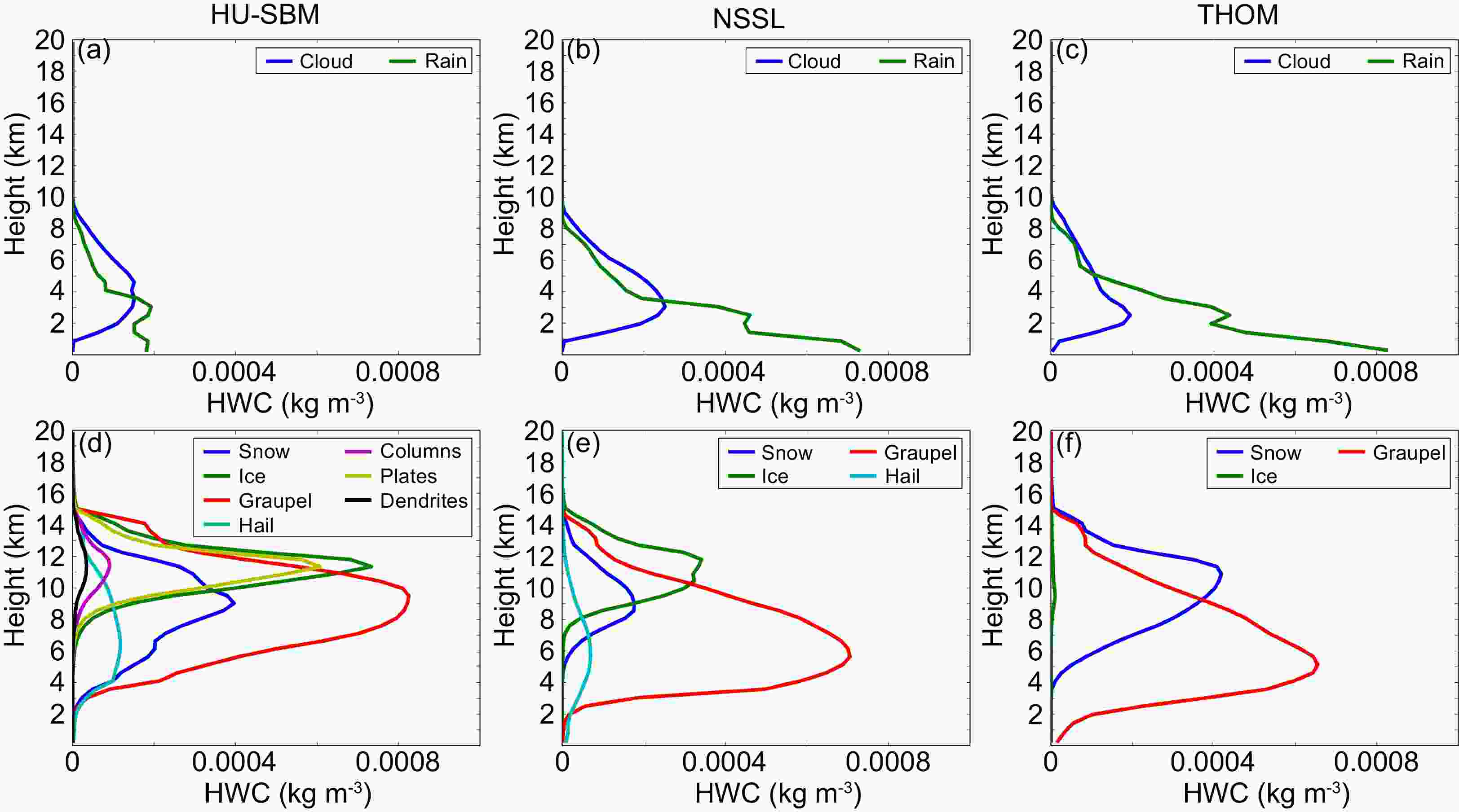
Figure 5. Vertical profiles of horizontally averaged hydrometeor water content (units: kg m−3) for (a–c) liquid and (d–f) ice hydrometeors for the (a, d) HU-SBM, (b, e) NSSL, and (c, f) Thompson microphysics schemes at t = 100 min.
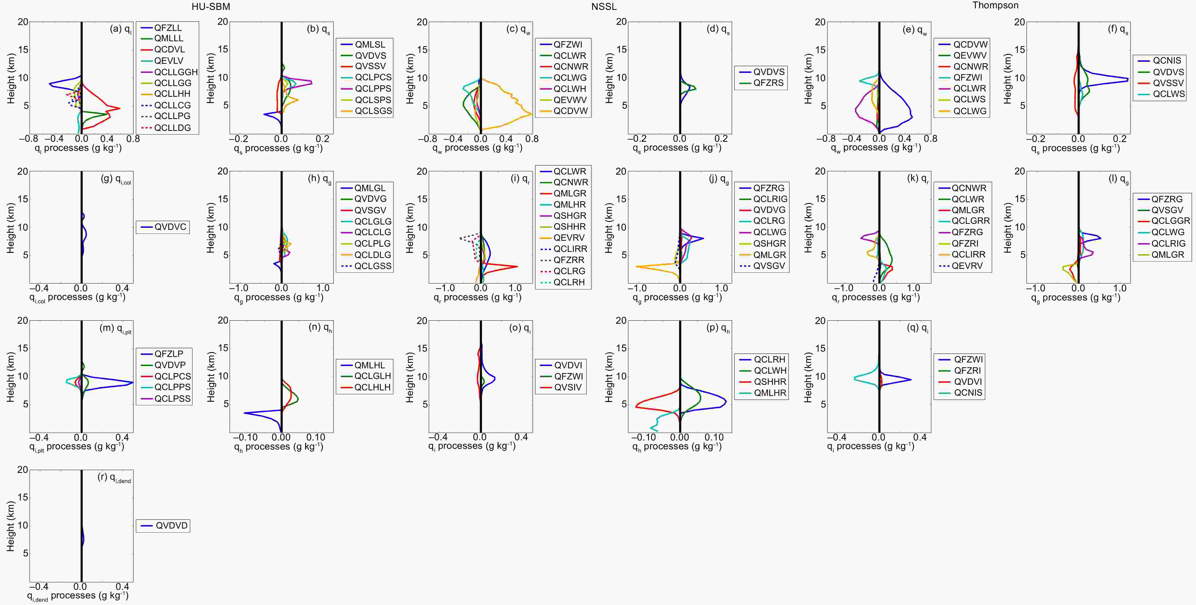
Figure 6. Vertical profiles of horizontally averaged 5-min accumulated mixing ratio process rates (units: g kg−1) for the (left two columns) HU-SBM, (middle two columns) NSSL, and (right two columns) Thompson microphysics schemes at t = 100 min. Plot labels indicate the relevant hydrometeor. The vertical black line in each plot denotes zero.
The rainwater content is much smaller in HU-SBM compared to those in NSSL and Thompson, which is also the case with the domain-averaged masses. The rainwater content in Thompson is generally larger than that in NSSL, similar to the domain-averaged masses. Both bulk simulations have their rainwater content peaks near the surface, while HU-SBM’s rainwater peaks near z = ~3 km. HU-SBM’s rain sources near this peak are presumably melting ice (both rimed ice and snow aggregates), but might include condensation as well. There are small HU-SBM sinks near this height. The rain sources in the BMP simulations (which are larger) are melting rimed ice and collection of cloud water (while Thompson includes rain collecting graupel). These processes peak above the surface, especially cloud water collection. Therefore, the heights of rain peaks in BMP simulations seem to be more related to sedimentation and storm downdrafts, which will be discussed later. We also note here that the low-level rain evaporation rates among the simulations are consistent with the cold pool intensities in Fig. 1 (i.e., Thompson’s rain evaporation is largest).
HU-SBM’s cloud ice water content peaks between z = 11 km and z = 12 km, primarily owing to the plate ice mass (Fig. 5d). This height is similar to that of the peak level of NSSL’s cloud ice (z = ~12 km; Fig. 5e), while Thompson’s ice peaks between z = 9 km and z = 10 km. The cloud ice of HU-SBM and NSSL is primarily created through freezing liquid (Figs. 6m and o). The lower cloud ice peak of the Thompson scheme is the result of its aggressive conversion of cloud ice to snow, especially above 10 km (Fig. 6q). Melting cloud ice does not contribute significantly to liquid in any of the microphysics simulations, which indicates its contribution to precipitation likely derives from conversion to other hydrometeors (e.g., conversion to snow and subsequently melting to rain, three-component freezing to graupel, etc.). Still, snow only noticeably makes it to the melting level in HU-SBM, as its vertical profile is near 0 kg m−3 in the NSSL and Thompson simulations. HU-SBM’s snow from snow–graupel collisions is larger than the snow sources in the BMP simulations near z = ~5 km (Figs. 6b, d and f), in addition to crystal and snow collisions above.
The graupel vertical profiles are noticeably different across the three simulations. For instance, the graupel water content peaks near z = 10 km in HU-SBM, while in the NSSL and Thompson simulations it peaks near z = 6 km and z = 5 km, respectively. While freezing rain provides similar graupel sources near z = 8 km for the bulk simulations, the Thompson scheme also contains a peak in cloud ice and rain freezing to graupel near z = 5 km (Figs. 6j and l). HU-SBM’s graupel is primarily created through crystal–liquid collisions below z = 10 km (Fig. 6h). While HU-SBM’s graupel HWC peak is larger than in the NSSL and Thompson schemes, it is not reflective of the large amount of graupel simulated over the duration of the simulated storm (Fig. 3). Again, HU-SBM’s condensate coverage is larger than in the bulk schemes (not shown). The weak downward graupel flux in HU-SBM inferred from its vertical profile hinders precipitation reaching the ground, as melting rimed ice is the primary source for low-level rain in these supercell simulations. HU-SBM’s hail water content peaks near z = 7 km, while in NSSL it peaks near z = 6 km and is able to reach the surface. HU-SBM’s hail is primarily created from graupel–liquid collisions near z = 6 km (Fig. 6n). NSSL’s hail forms mostly from graupel conversion (Fig. 4), and experiences more wet growth than in the HU-SBM simulation (Figs. 6n and p), allowing for greater hail growth potential despite its large shedding. HU-SBM’s hail melting occurs faster than NSSL’s hail in the melting layer, suggesting either a larger hail size in NSSL and/or greater downward hail transport.
-
The vertical transport of hydrometeors at a mature supercell stage (t = 100 min) is further investigated to elaborate on the roles of storm kinematics, parameterized fall speed, PSD parameterizations, and underlying MP hydrometeor production with regard to precipitation near the surface. The updraft/downdraft HWC flux (defined here as ρwqx), hydrometeor sedimentation (defined as −ρvtqx), and the net vertical hydrometeor flux [ρ(w − vt)qx] are utilized to analyze these roles, where ρ is the ambient air density, qx is the mixing ratio of hydrometeor x (e.g., rain), w is the vertical velocity of the updraft/downdraft, and vt is the mass-weighted mean terminal velocity calculated from each scheme’s fall speed parameterization. All fluxes are averaged at each vertical level over the horizontal domain where the condensate mixing ratio exceeds 0.01 g kg−1 (Fig. 7). Cloud water and ice are not included given their generally small fall speed.
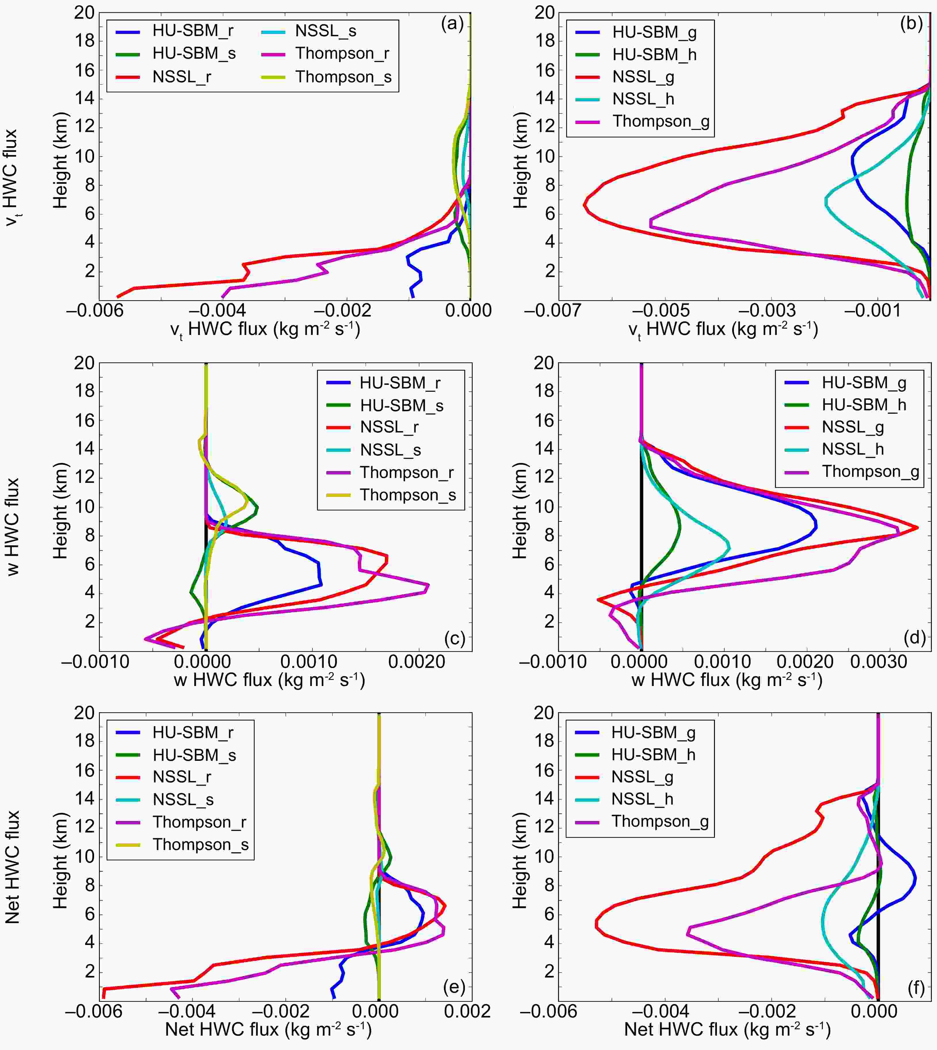
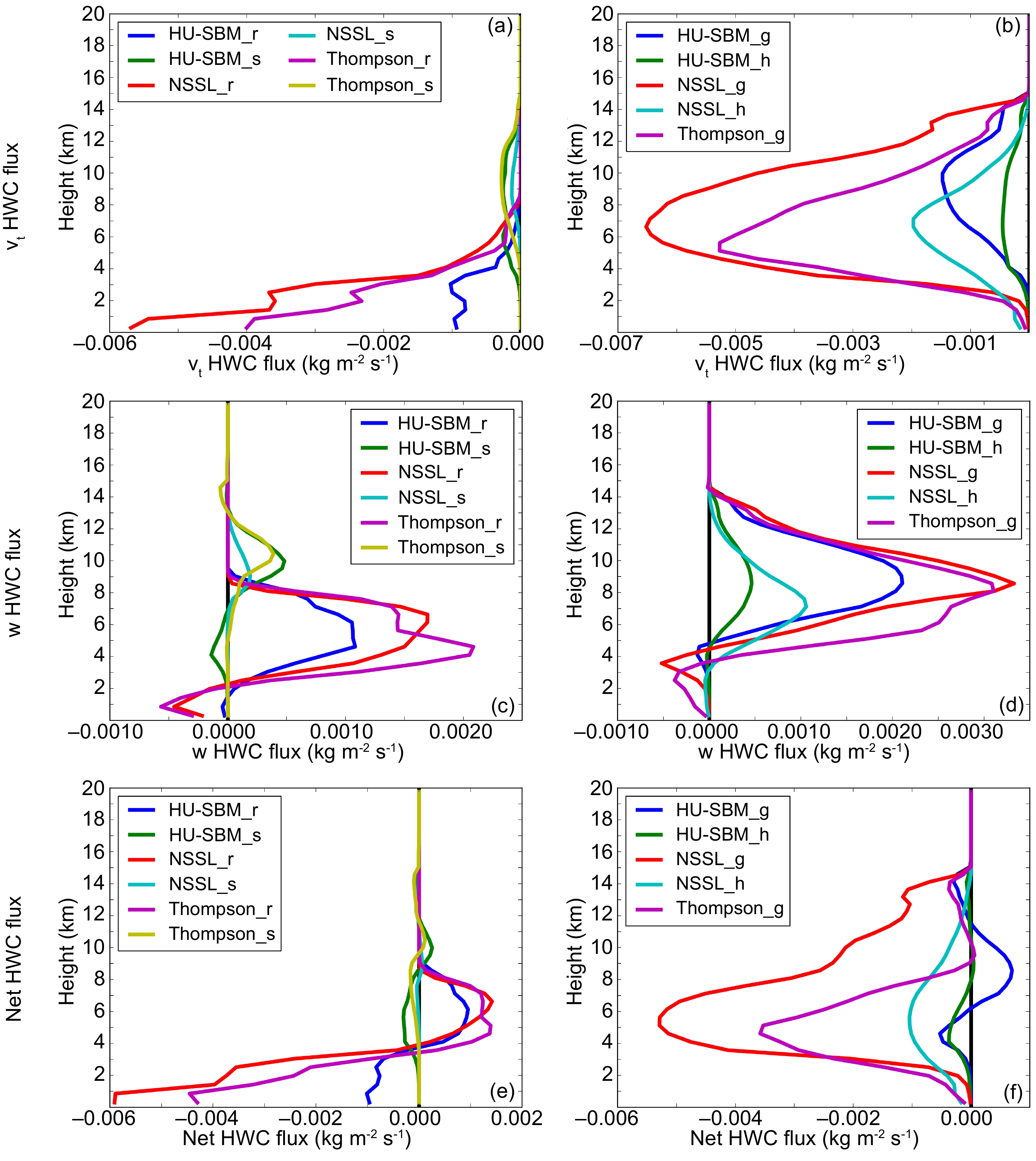
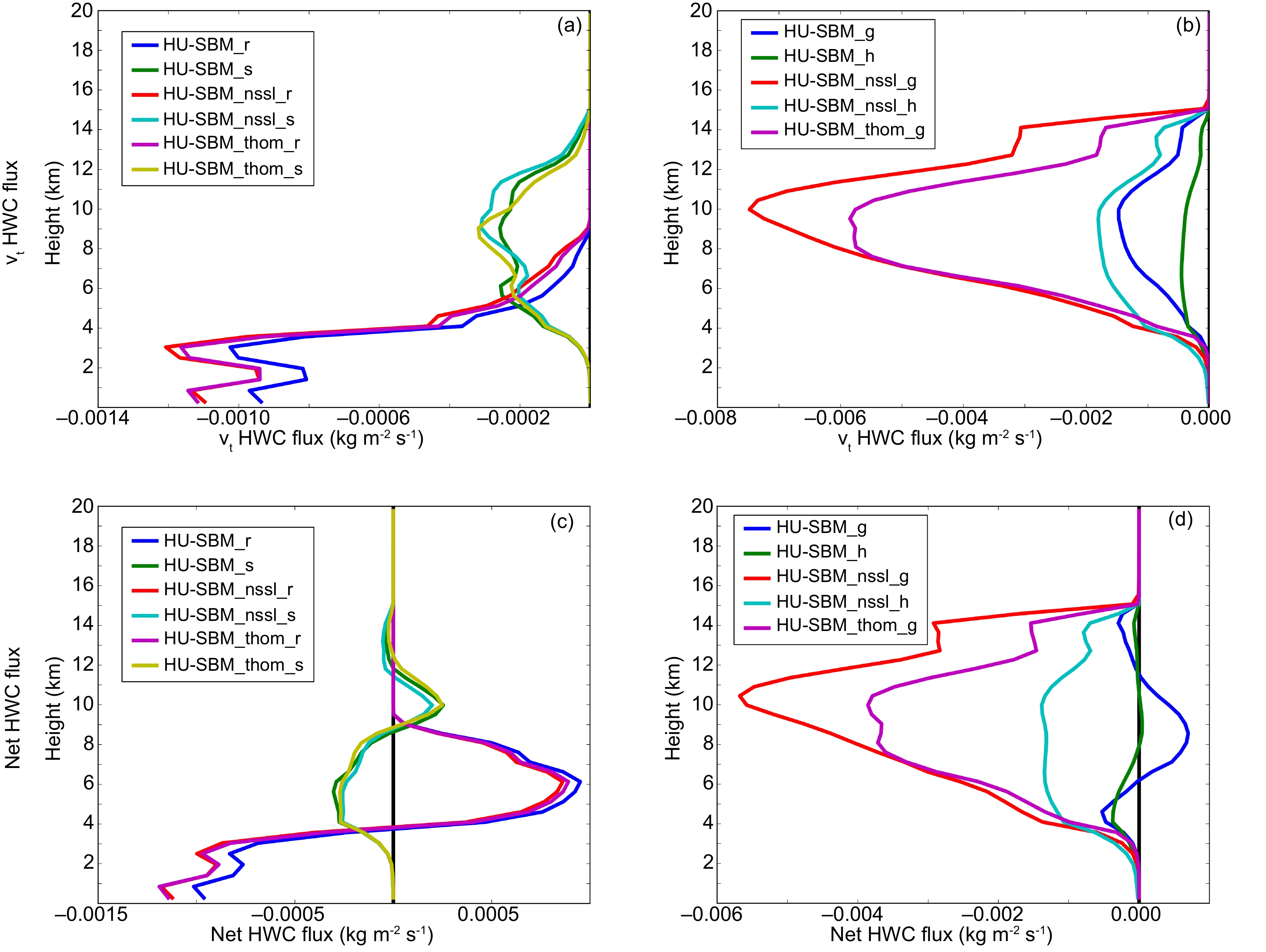
Figure 7. Vertical profiles of horizontally averaged hydrometeor water content fluxes (units: kg m−2 s−1) calculated with (a, b) mass-weighted mean hydrometeor fall speed (vt), (c, d) updraft/downdrafts (w), and (e, f) their net (w – vt) vertical speed for (a, c, e) rain and snow, and (b, d, f) graupel and hail hydrometeors at t = 100 min. PSDs and fall speeds to calculate vt are consistent with each microphysics scheme’s parameterizations.
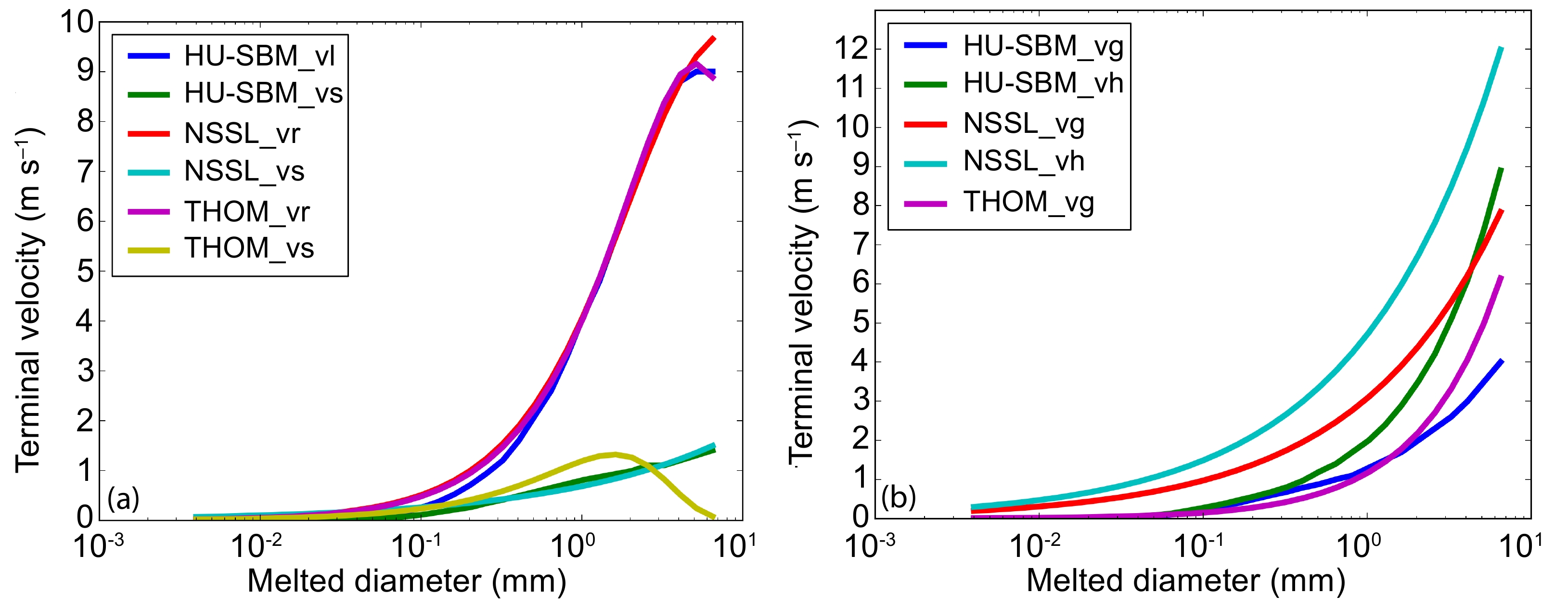
NSSL’s rain sedimentation flux generally has larger magnitude than that of the Thompson scheme below z = ~7 km (Fig. 7a). While neither scheme’s HWC is definitively larger over this depth (Fig. 5b and c) and their rain fall-speed relationships are similar (Fig. 8a), NSSL’s maximum rain vt is larger than that of Thompson below z = ~8 km (not shown). Both bulk rain sedimentation fluxes have larger magnitude than in HU-SBM, which is a consequence of HU-SBM’s comparatively small rainwater content. As Thompson’s snow fall-speed is slightly larger for melted particle diameters < ~2.5 mm (Fig. 8a), its generally larger snow mass results in a larger snow sedimentation flux above z = 7–8 km, below which the larger snow mass of HU-SBM results in a greater sedimentation flux (Fig. 7a). Downdrafts (negative w) containing rain and snow (Fig. 7c) contribute to downward net snow flux near and above the melting level and net rain fluxes near the surface (Fig. 7e). The downward net snow flux in HU-SBM is larger than in the bulk simulations near the melting level, but likely does not contribute directly to precipitation given its small magnitude. HU-SBM’s rain has a smaller downward net flux near the surface compared to the two bulk simulations, partially due to weaker downdrafts. The NSSL simulation’s largest downward net rain flux near the surface helps explain the scheme’s largest accumulated precipitation (Fig. 2).
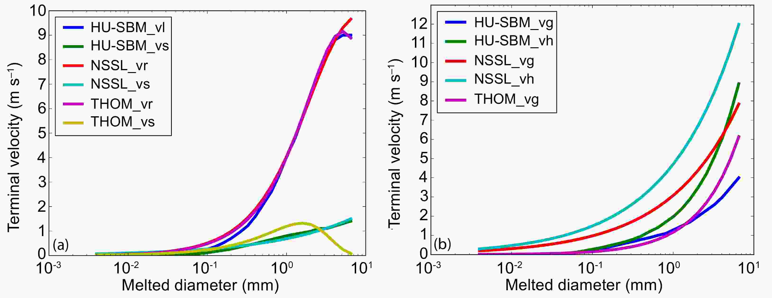
Figure 8. Terminal velocities (units: m s−1) spaced by HU-SBM mass bins [but shown here relative to melted diameter (units: mm)] of (a) rain (or HU-SBM liquid) and snow, and (b) graupel and hail, in the HU-SBM, NSSL, and Thompson schemes. The “_vx” suffix denotes the relationship for hydrometeor x. Terminal velocities are plotted in each microphysics scheme’s reference state (i.e., pressure = 1000 hPa in HU-SBM, air density ρa = 1.225 and 1.185 kg m−3 in the NSSL and Thompson schemes, respectively). NSSL graupel and hail fall speeds are displayed with bulk densities of ρg = 500 and ρh = 900 kg m−3, respectively.
HU-SBM’s rimed ice sedimentation flux is smaller than those of the bulk simulations (Fig. 7b), even though its graupel and hail HWC peaks in the vertical profiles are largest. Its rimed ice fall speeds are smaller than those in NSSL (for equal constant density; not shown), and its graupel fall speed is progressively smaller than Thompson’s graupel for melted particle sizes > ~1.5 mm (Fig. 8b), slowing its downward rimed ice transport. While upward rimed ice fluxes are large (Fig. 7d), large sedimentation fluxes in the bulk simulations result in overwhelmingly downward net rimed ice fluxes (Fig. 7f). HU-SBM’s net graupel flux is upward between z = 6 km and z = 11 km, a result of its slower fall speeds compared to the NSSL and Thompson schemes. Although Thompson’s graupel fall speed is smaller than that of NSSL’s graupel up to ice particle sizes of ~15 mm (for equal constant density; not shown), its larger graupel HWC (and typically larger downward transport in stronger downdrafts compared to HU-SBM and NSSL) provides a generally greater net flux below the melting level. HU-SBM’s hail also has a weaker downward net flux compared to NSSL’s hail, due to faster hail fall speeds in NSSL (Fig. 8b) and stronger downdrafts. The rimed ice contribution to precipitation can also be demonstrated below z = ~4 km, where the net rimed ice flux of each simulation decreases due to melting (although bulk net fluxes are larger).
-
The vertical fluxes of hydrometeors are further analyzed by examining their sensitivity to terminal velocity and bin/bulk PSD parameterization. This is performed in an offline mode, using hydrometeor model fields simulated by the original simulations at a mature stage (t = 100 min). To calculate the mass-weighted mean terminal velocities vt using a bulk scheme formulation from the bin scheme–predicted hydrometeors, the bulk fall-speed formulations are employed and the bulk PSDs are diagnosed using the total bulk mass mixing ratios and number concentrations that were summed over the HU-SBM bins. To calculate vt using HU-SBM’s formulations for the NSSL and Thompson schemes, the bulk hydrometeor species are discretized into 33 mass bins based on their assumed PSDs (from their bulk mass and number concentrations), and then the HU-SBM fall-speed formulations are used. The vertical velocities from the original simulations are used for vertical hydrometeor transport by updrafts/downdrafts.
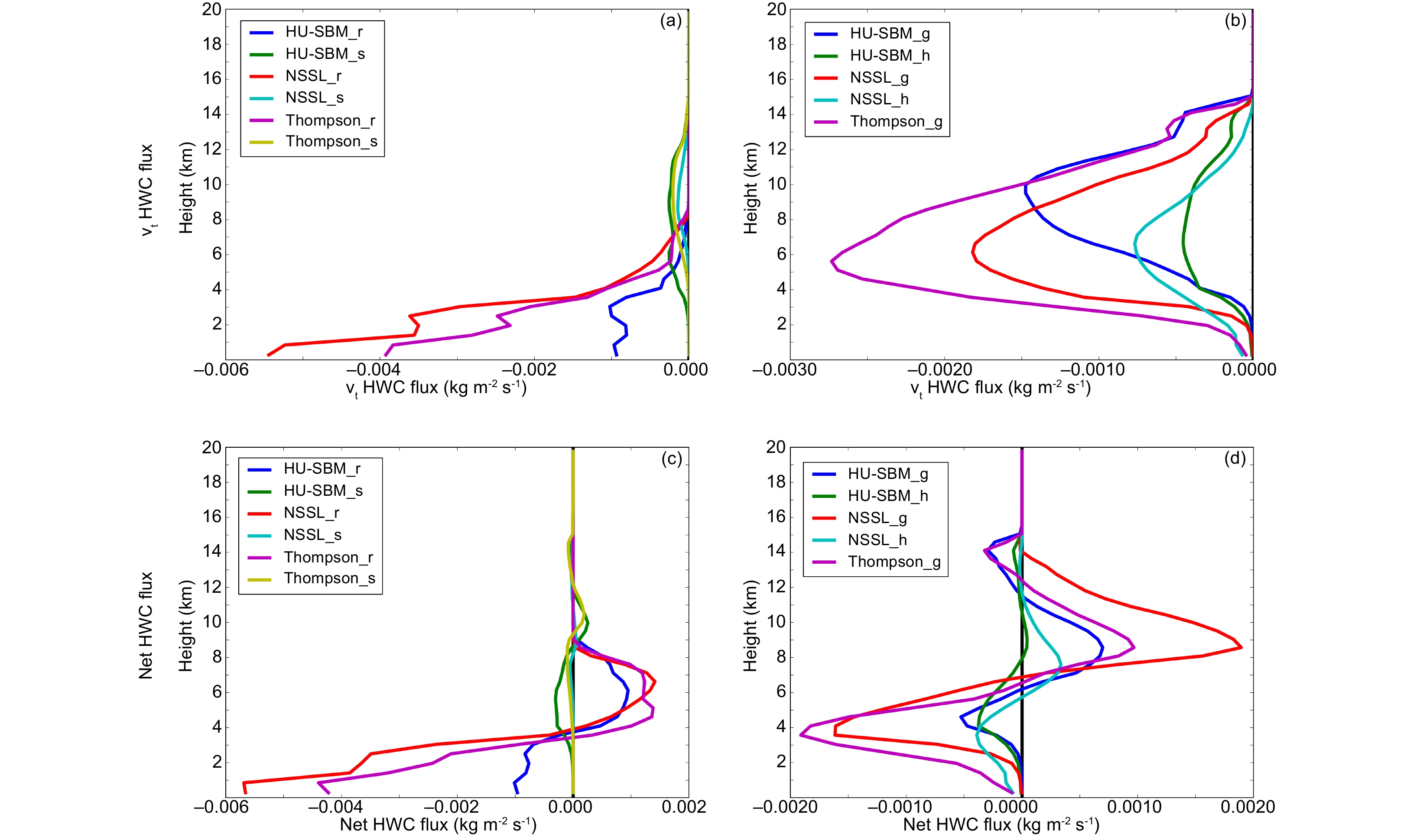
Calculating the rain sedimentation flux using the NSSL and Thompson fall-speed formulations and treating HU-SBM’s rain as bulk rainwater increases the sedimentation flux relative to the flux using the native formulation (Fig. 9a). In the bulk framework, HU-SBM’s rain now effectively has a smooth PSD across all diameters and is rid of its maximum mass limitation. Both bulk schemes assume an exponential distribution of rain with very similar fall speeds (Fig. 8a), highlighting the effects of PSD parameterization on rain flux. Increasing HU-SBM’s rain sedimentation flux also increases its downward net flux toward the surface and reduces its upward flux (Fig. 9c). HU-SBM’s sedimentation and net rain fluxes calculated from the NSSL and Thompson fall speeds and bulk PSD assumptions are still smaller in magnitude than the sedimentation and net rain fluxes of NSSL and Thompson near the surface. This is related to the underlying HU-SBM rain mass field dictated by HU-SBM’s liquid processes (i.e., melting ice particles), resulting in a smaller rain HWC vertical profile compared to the bulk simulations (Figs. 5a–c). HU-SBM’s snow sedimentation flux is generally unchanged near the melting level using the NSSL and Thompson bulk formulations. Although the snow fall speeds of NSSL and Thompson can be faster than those of HU-SBM, constraining HU-SBM to a fixed PSD shape has the potential to introduce more small snow particles. As a result, HU-SBM’s net snow flux is also similar near the melting level when using the NSSL and Thompson bulk formulations.
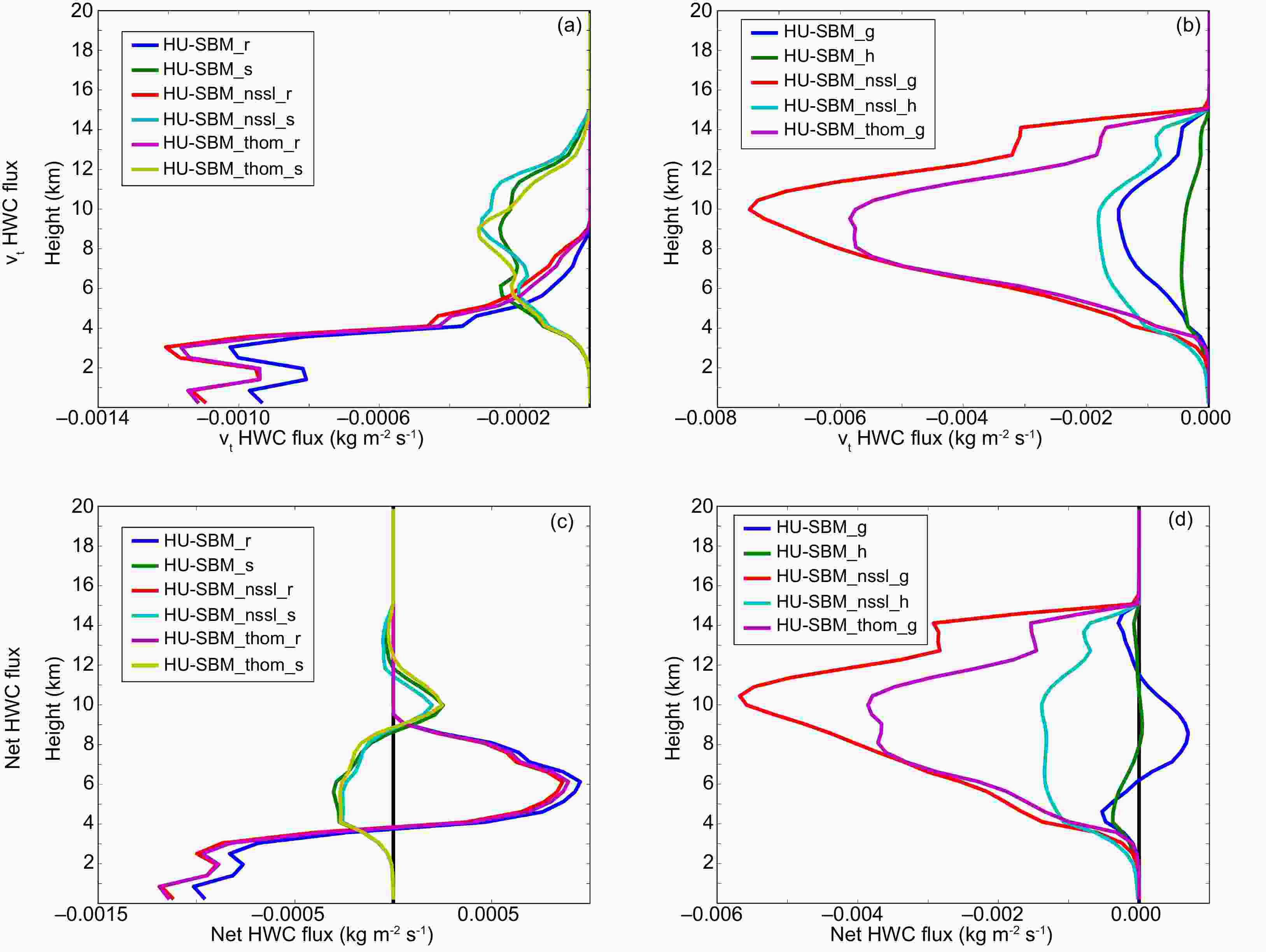
Figure 9. Vertical profiles of horizontally averaged hydrometeor water content fluxes (units: kg m−2 s−1) calculated with (a, b) mass-weighted mean hydrometeor fall speed (vt), and (c, d) their net (w – vt) vertical speed for (a, c) rain and snow, and (b, d) graupel and hail hydrometeors at t = 100 min. HU-SBM PSDs and fall-speed parameterizations to calculate vt follow original HU-SBM parameterizations (HU-SBM_x), or those in the NSSL (HU-SBM_nssl_x) or Thompson (HU-SBM_thom_x) schemes for hydrometeor x.
Replacing HU-SBM’s graupel and hail bins and fall speeds with NSSL’s fall speeds and bulk PSD assumptions (from HU-SBM’s q and NT) significantly increases each category’s sedimentation flux (Fig. 9b). The rimed ice fall speed in the NSSL scheme exceeds that of HU-SBM (for equal constant density; not shown), increasing its downward transport. Using Thompson’s bulk graupel assumptions also increases HU-SBM’s graupel sedimentation flux, although not as much as in NSSL. Thompson’s graupel fall speed is typically smaller than that of NSSL (Fig. 8b). Increasing the rimed ice sedimentation expectedly increases its downward net flux (Fig. 9d), although HU-SBM’s underlying rimed ice production within the simulation precludes net flux increases near the surface relative to NSSL’s hail and Thompson’s graupel. Therefore, while increasing fall speeds in the HU-SBM scheme would increase surface precipitation, precipitation differences across the three microphysics schemes cannot be attributed to fall speed alone.
The NSSL and Thompson rain and snow sedimentation fluxes change subtly when the NSSL and Thompson bulk PSDs are discretized into HU-SBM’s 33 mass bins and the fall-speed formulations of HU-SBM are used in each bin (Fig. 10a). The rain sedimentation fluxes near the surface are reduced slightly in the two bulk simulations. The rain fall-speed relationships are similar among the three schemes (although HU-SBM’s liquid fall speed is slightly slower for drops < 1 mm; Fig. 8a), while HU-SBM’s mass bin discretization contains a maximum rain diameter of 6.5 mm, corresponding to very large raindrops. Thompson’s snow sedimentation flux is slightly reduced, likely attributable to the generally slower HU-SBM fall speed. Therefore, Thompson’s net snow flux above the melting level, and the near-surface NSSL and Thompson net rain fluxes, are slightly reduced (Fig. 10c), but their near-surface net rain fluxes are larger than in the HU-SBM simulation.
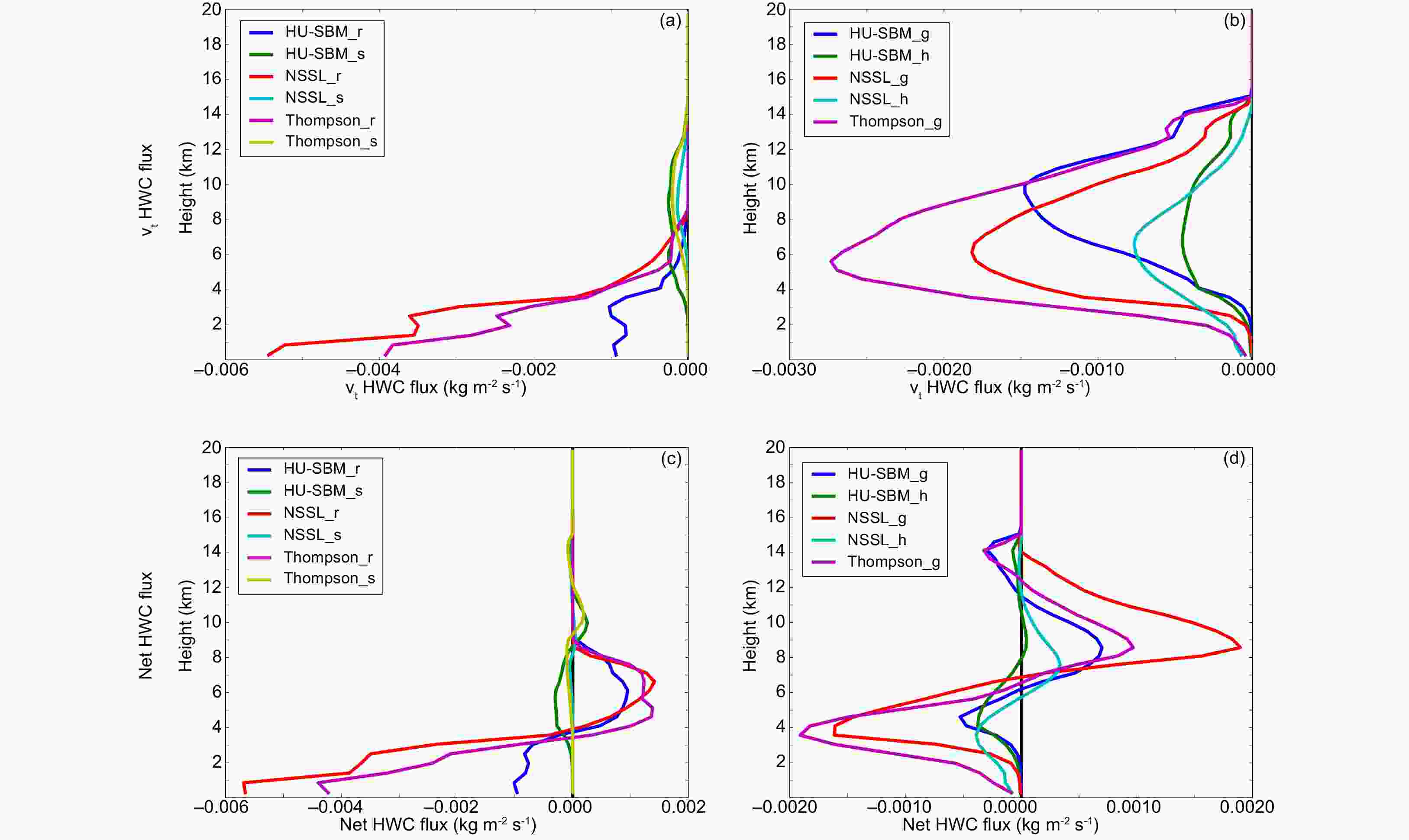
Figure 10. As in Fig. 9 but with NSSL and Thompson PSDs and fall-speed parameterizations following those in the HU-SBM scheme.
In contrast, the rimed ice sedimentation fluxes are reduced significantly for NSSL and Thompson but are still generally larger than those of HU-SBM’s rimed ice below z = ~9 km (Fig. 10b). These reductions can be attributed to slower HU-SBM rimed ice fall speeds relative to those of NSSL, and for melted particles larger than 1.5 mm relative to Thompson’s graupel fall speeds. Another contributing factor could be the maximum mass bins of HU-SBM corresponding to the NSSL and Thompson graupel sizes (at ρg = 500 kg m−3) being equal to 8.19 mm, and NSSL’s hail size (at ρh = 900 kg m−3) being equal to 6.73 mm, reducing the calculated vt due to the truncated PSDs. Again, the rimed ice density in the NSSL is predicted. The resulting increase in upward net flux and decrease in downward net flux of rimed ice to the melting level (Fig. 10d) would reduce rimed ice melting to rain, and subsequently surface precipitation.
-
Idealized supercell simulations are performed in this study using the HU-SBM “full” spectral bin, and NSSL and Thompson bulk MP schemes available within WRF version 3.7.1. The HU-SBM simulation produces much less precipitation than the two bulk simulations over the 2-h simulations, and the behaviors of the schemes in the simulations are analyzed to investigate the main reasons for the precipitation differences. Domain-averaged and vertical profiles of process rates from the different simulations, as well as hydrometeor mass, water content, and vertical fluxes for different species, are examined.
Over the 2-h duration of the simulated storm, the HU-SBM scheme simulates more cloud ice (plates), graupel, and hail, but less rainwater than the bulk simulations. HU-SBM appears to aggressively freeze large amounts of liquid to plate crystals, which can then aggregate to snow or freeze (along with other crystals) with liquid to graupel. Thompson simulates a large amount of snow mass, similar to that in HU-SBM, due to the scheme’s aggressive cloud ice–snow conversion. Graupel in the bulk simulations is primarily sourced from freezing rain, with additional contributions from cloud ice and rain freezing to graupel in the Thompson simulation. The larger HU-SBM graupel HWC peak above the NSSL and Thompson graupel peaks in their vertical profiles (at a mature stage in the simulations; t = 100 min) reflects its maximum mass bin limiting larger particles during three-component freezing or wet growth. Smaller rimed ice particles combined with slower fall speeds lead to quicker updraft ejection. HU-SBM’s hail experiences less wet growth than NSSL’s, which may be due to, or reflective of, a shorter updraft residency time.
The primary source of rain near the surface is from melting rimed ice, although HU-SBM additionally includes melting snow aggregates and the Thompson simulation includes rain collecting graupel. The lower HU-SBM rainwater amount near the surface is due to a greater contribution of slower-falling snow (itself sourced from ice crystals, snow, and graupel collisions) to rain compared to those in the bulk schemes, along with the previously mentioned maximum mass bin limiting rimed ice particle sizes, and generally slower rimed ice fall speeds than those of the bulk schemes. Downward water mass transport is further complicated by HU-SBM’s weakest downdrafts among the schemes, consistent with its smallest low-level evaporation rate.
In offline calculations for a single time (t = 100 min) at a mature stage of simulation, HU-SBM produces the smallest downward net rain flux to the surface because of its lowest rainwater content and weaker downdraft flux. This is likely due to a combination of net snow flux near the melting layer that is larger than those in the bulk simulations, and the smallest net graupel and hail fluxes at the melting level and surface. The smaller HU-SBM rimed ice net fluxes reflect generally slower rimed ice fall speeds and weaker downdraft fluxes. The NSSL simulation has a larger net rain flux to the surface than that in Thompson, explaining its largest precipitation among the three simulations.
Downward net fluxes of rain and rimed ice for HU-SBM are increased when they are calculated using the fall-speed formulations of the NSSL and Thompson bulk schemes. When doing so, the discretized PSDs of HU-SBM are replaced with bulk PSDs (e.g., exponential or gamma distributions) by summing over the spectral bins to calculate q and NT. The net rain fluxes near the surface are still smaller than those in the bulk simulations, while the net rimed ice fluxes near the surface are smaller than NSSL’s hail and Thompson’s graupel net fluxes. This can be attributed to the underlying smaller amounts of qr, qg, and qh as seen in their vertical profiles. Conversely, discretizing the moment-based bulk PSDs in the NSSL and Thompson schemes and calculating the fall speeds for the discretized bins using HU-SBM’s fall-speed formulations reduces the near-surface downward net rain fluxes slightly (due to the slightly smaller HU-SBM fall speed and a maximum rain mass bin limiter). The downward net flux of rimed ice to the melting layer is also reduced, owing to the restrictive maximum rimed ice mass bins employed and typically smaller rimed ice fall speeds in the HU-SBM scheme. Still, the higher rain and rimed ice contents simulated by the bulk simulations (aided by stronger downdrafts) allow their downward net fluxes to typically exceed those in HU-SBM to the melting layer and surface.
We have demonstrated that, in a supercell framework, precipitation differences between MP schemes are more complex than just differences in simulated rainwater content or hydrometeor fall speeds. Understanding the main causes of the differences requires detailed analyses to gain insight on hydrometeor conversions/growth, interactions with storm dynamics (i.e., cold pool and updrafts/downdrafts), and subsequent vertical transport of hydrometeors. An important consideration for SBMs is the number of hydrometeor mass bins, to allow for sufficient rimed ice growth within the scheme, especially for intense deep convection. Supercell storms tend to produce a large amount of rimed ice particles that contribute significantly to precipitation production. Adequate rimed ice wet growth facilitated by fast rimed ice fall speeds can ensure greater ice mass flux to the melting level and eventually to the surface after melting. Significant snow contribution to precipitation in supercells may be problematic and may require particle evolution adjustment (such as enhancing riming/wet growth given the large amount of plates from freezing liquid by HU-SBM that generally aggregate to snow, reducing snow–graupel collisions that convert graupel to snow), as snow particles sediment much slower than rimed ice. More rain in the melting layer sourced from rimed ice may provide dynamic feedback by strengthening downdrafts through evaporation, resulting in more negatively buoyant air. Such insights are valuable to NWP researchers for model tuning, given the complexity of MP schemes from hydrometeor creation to surface precipitation. Comparisons of real-case supercell simulations to observations may further refine supercellular process representations and parameterizations by comparing the simulation with available observations. This is a subject for future work.
Acknowledgements. This research was primarily supported by a NOAA Warn-on-Forecast (WoF) grant (Grant No. NA16OAR4320115). We thank the two anonymous reviewers, whose feedback improved the quality of this manuscript.
| WRF model configuration | |
| Run time | 120 min |
| Δt | 6 s |
| Sound wave Δt | 1 s |
| Model output interval | 10 min |
| Horizontal domain | 200 km × 200 km |
| Model lid | 20 km |
| Δx | 1 km |
| Δy | 1 km |
| Δz | ~500 m |
| Time integration scheme | Third order Runge–Kutta |
| Horizontal momentum advection | Fifth order |
| Vertical momentum advection | Third order |
| Horizontal scalar advection | Fifth order |
| Vertical scalar advection | Third order |
| Upper level damping | 5000 m below model top |
| Rayleigh damping coefficient | 0.003 |
| Turbulence | 3D 1.5-order turbulent kinetic energy closure |
| Horizontal boundary conditions | Open |
 AAS Website
 AAS WeChat