


 DownLoad:


-
Due to the development of atmospheric radiative transfer models and data assimilation (DA) techniques, satellite data have become one of the main sources of observations used in numerical weather prediction since the 1990s (Derber and Wu, 1998; Shi et al., 2021). According to the European Centre for Medium-Range Weather Forecasts, satellite data account for more than 90% of all data used for assimilation (Bauer et al., 2010). Typhoons pose great threats to people’s lives and to economies in coastal areas all over the world every year (Pielke and Landsea, 1998; Shen and Min, 2015; Shen et al., 2021a, b; Zhou et al., 2021; Song et al., 2022), but their formation and evolution happens mostly over open ocean where conventional observations are sparse. In recent years, it has been found that assimilating radiances from geostationary satellites has the ability to improve the forecasting of typhoons since they are able to provide almost continuous four-dimensional information about the atmosphere. For example, Zou et al. (2015) and Zhang et al. (2016) directly assimilated imager radiances from the Geostationary Operational Environmental Satellite and achieved drastic improvements in terms of the thermodynamic fields, such as temperature and moisture, as well as the dynamic fields, including wind and geopotential, thus reducing the forecast errors of the track and intensity of tropical cyclones. Minamide and Zhang (2018) and Honda et al. (2018) assimilated the all-sky infrared radiances from Himawari-8 with a convection-permitting scale at 10-min intervals to capture the rapid intensification process of Super Typhoon Soudelor (2015) in a numerical model.
However, due to the uncertainty in cloud and precipitation data (Bauer et al., 2006; Kim et al., 2010; Geer and Bauer, 2011; Okamoto et al., 2014; Zhang et al., 2016, 2022c; Xian et al., 2019; Xu et al., 2021; Li et al., 2022b; Zhu et al., 2022), usually, only infrared radiances unaffected by cloud are assimilated, meaning clear-sky assimilation has been widely used both operationally and in scientific research (Hoppel et al., 2013; Kazumori, 2014; Jones et al., 2018; Wang et al., 2018; Zhu et al., 2019; Shen et al., 2021a, b). Detection of “clear radiance” suitable for clear-sky DA is crucial (McNally, 2002). The common approach is to utilize imagers from visible and near-infrared channels to determine pixels affected by clouds (Ackerman et al., 1998). For example, Gao et al. (2003) discovered that the 1.38-µm near-infrared channel of MODIS can be applied to detect high clouds in the polar region during daytime. Another widely used group of cloud detection schemes involves distinguishing cloudy and clear pixels by the difference in the observed radiance and the equivalent clear-sky radiance (Smith and Frey, 1990). Huang et al. (2004) proposed the minimum local emissivity variance technique to obtain the optimal estimation of single-layer cloud emission by calculating the local variance of the cloud spectral emissivity of a specific pressure layer in the background field. McNally and Watts (2003) proposed a method to detect cloud using high-spectral infrared sounders radiances and reported a residual of less than 0.2 K. Based on the variational method, Auligné et al. (2014a, b) presented the multivariate and minimum residual (MMR) method to retrieve three-dimensional cloud fractions so as to conduct cloud detections, in which the minimization method is used to fit the observation and the cloud conditions of each model layer are retrieved via building the cost function (Xu et al., 2014, 2015). Based on the particle filter (PF) algorithm (van Leeuwen, 2010; Karlsson et al., 2015), Xu et al. (2016) developed a cloud detection method comparable to the MMR method since both methods originally need to retrieve cloud fractions. It was found that cloud retrievals from both schemes are rather consistent, and the PF scheme is more computationally efficient. Although studies on cloud retrieval or detection are well-established and have achieved promising results with the PF and MMR methods, the impacts of these different cloud detection schemes on satellite radiance DA, especially in typhoon initialization, needs further investigation.
China’s FY-4 series of satellites are the country’s second generation of geostationary meteorological satellites. As the pioneering satellite, FY-4A was launched on 11 December 2016 and put into operation on 1 May 2018. It is located above the equator at 104.7°E and adopts three-axis stabilization for control. Compared with the first generation FY-2 series, the temporal resolution has doubled, providing a full-disc scan every 15 min, which is beneficial for monitoring rapidly developing mesoscale synoptic systems (Yang et al., 2017). It is equipped with several advanced instruments, including the Advanced Geosynchronous Radiation Imager (AGRI), the Geostationary Interferometric Infrared Sounder, the Lightning Mapping Imager, and the Space Environment Package. Among them, the performance of AGRI is much better than that of the infrared radiometer loaded on the first generation FY-2 series satellites, in terms of higher temporal and spatial resolution (Zhang et al., 2019, 2022a; Niu et al., 2023). Researchers have mainly focused on the calibration, quality estimation, and precipitation retrieval with AGRI data (Wang et al., 2020; Zhu et al., 2020; Hu et al., 2021; Tang et al., 2021; Yu et al., 2021; Xu et al., 2022, 2023; Zhang et al., 2022b). However, the application of AGRI radiance DA, especially in typhoon initialization, is less well studied.
In this paper, therefore, we present the impact on typhoon forecasts of assimilating clear-sky FY-4A AGRI radiances of two water vapor channels with a channel-sensitive cloud detection scheme based on the PF algorithm after implementing the interface of FY-4A AGRI radiance assimilation. To the best of our knowledge, the application of FY-4A AGRI DA in typhoon predictions has scarcely been studied and is thus worthy of in-depth investigation. Based on multiple typhoon cases, the mechanism of improvement in analyses and forecasts of typhoons is also discussed.
The rest of the paper is arranged as follows: Section 2 gives a brief introduction to the radiance DA methods, including the different cloud detection schemes, quality control, and bias correction. Section 3 provides details of the typhoon cases, the features of the FY-4A AGRI radiance, and the experimental design. Analysis and forecast verification of the typhoons is presented in section 4, followed by conclusions and future perspectives in section 5.
-
In this study, the 3DVar DA method of the WRFDA system is adopted (Barker et al., 2012). To obtain the best estimate of the atmospheric state, the 3DVar assimilation method minimizes a scalar cost function,
where
$ {\bf{x}} $ is the analysis vector,$ {{\bf{x}}_{\mathrm{b}}} $ is the background vector,$ {{\bf{y}}_0} $ is the observation vector,$ {\mathbf{B}} $ is the background error covariance, and$ {\mathbf{R}} $ is the observation error covariance.$ H $ is the observation operator to project variables from the model space to the observation space. Radiative Transfer for Television and Infrared Observation Satellite (RTTOV; Saunders et al., 2018) is the radiative transfer model used in this study for AGRI radiance DA. In the following experiments, National Meteorological Center method (Parrish and Derber, 1992) with one-month forecasts is applied to generate the background error covariance and the CV5 (control variable option 5) scheme is employed with the stream function (ψ) and the potential function (φ) as momentum control variables (Lorenc et al., 2000; Wu et al., 2002). Other control variables include the unbalanced temperature, the pseudo relative humidity, and the unbalanced surface pressure. -
In this study, two channel-dependent cloud detection schemes based upon the PF and MMR methods are each compared with a pixel-based cloud detection scheme with a cloud mask product. Former applications of the PF and MMR algorithms mainly focused on cloud retrieval, rather than on cloud detection, to select channels for DA. Therefore, the investigation of the impact of these two cloud detection schemes on DA is novel for clear-sky infrared radiance DA.
-
Based on the Monte Carlo method (Doucet et al., 2001; Arulampalam et al., 2002), the PF algorithm is a sequential importance sampling method that gives the distribution of random state particles extracted from their posteriori probability (Poterjoy, 2016; Xu et al., 2016; Feng et al., 2020).
In a field of view, assuming the model is divided into K levels,
$ {c_{{\text{b,}}1}} $ ,$ {c_{b,2}} $ , …,$ {c_{b,K}} $ are used to represent the vertical effective cloud fractions$ {C_{\text{b}}} $ in the background for each model layer. In particular,$ c{}_{b,0} $ is the background fraction of the clear sky. By this definition, the requirement that each cloud fraction in the background meets is as follows:The prior knowledge of the initial state is given by the probability distribution p(
$ {c_{\mathrm{b}}} $ ) based on the pre-assigned samples$ {C_{{\mathrm{b}},i}} $ ($ \forall i \in [1,n] $ ). Here, n is particle sample size. To be specific, one cloud profile corresponds to one particle. In this study, the initial particles are discretized by setting the one-layer cloud with a value from 100% to 0% (e.g., 100%, 90%, 80%, …, 0%, with 10% as the interval). In a Bayesian con text, the aim is to estimate the filtering distribution p($ {C_{\text{a}}} $ |$ {\mathrm{R}}{\text{a}}{{\text{d}}_{{\mathrm{obs}},\nu }} $ ) given all the observations$ {\mathrm{R}}{\text{a}}{{\text{d}}_{{\mathrm{obs}},\nu }} $ . To be specific,$ {\mathrm{R}}{\text{a}}{{\text{d}}_{{\mathrm{obs}},\nu }} $ is the observed radiance at wavenumber$ \nu $ . Assuming the model is divided into K levels, the simulated cloud$ {\mathrm{R}}{\text{a}}{{\text{d}}_{{\mathrm{cloud}},\nu }} $ is defined aswhere
$ {\mathrm{R}}{\text{a}}{{\text{d}}_{0,\nu }} $ is the simulated clear-sky radiance. A cost function Jo is defined for each particle i to measure how the particle fits the observation:The final analyzed cloud fraction
$ {c_{{\text{a}},k}} $ is updated by the product of$ {c_{{\text{b}},k}} $ and its corresponding posteriori probability, aswhere
$ \forall k \in [0,K] $ ,$ \sigma $ is the specified observation error, and$ {\mathrm{R}}{\text{a}}{{\text{d}}_{k,\nu }} $ is the simulated radiance of the blackbody cloud at wavenumber$ \nu $ at the kth layer of the model. It should be pointed out that the posteriori probability is assumed to follow a Gaussian distribution to feasibly measure the gap between the observation and background information in Eq. (4), although Gaussian distributions of the background and observations are not necessarily required in the PF method. However, a Gaussian PF is also known to be efficient because of its approximation of the posteriori distributions by single Gaussian distributions (Kotecha and Djuric, 2003). To satisfy the constraint of Eq. (2), the final analyzed cloud fractions$ {c_{{\text{a}},k}} $ are normalized by the following formula: -
The MMR method retrieves the effective cloud fraction of each model layer by minimizing the residual of the observed and simulated radiances (Auligné, 2014a, b; Xu et al., 2015). Assuming the model is divided into K levels, the simulated cloud
$ {\mathrm{R}}{\text{a}}{{\text{d}}_{{\mathrm{cloud}},\nu }} $ is defined asThe variational minimization method is adopted to gradually fit radiance observations to obtain the cloud information of the kth model layer by building the following cost function:
It should be noted that both cloud detection methods are conducted based on the two water-vapor infrared and four longwave infrared channels by modeling the cloud in a simple way for each pixel, although only the two water-vapor infrared channels are assimilated. Once the cloud fractions are determined, the cloud detection for each channel is performed afterward. That is, radiances are identified as clear when
$ \left| {{\mathrm{R}}{\text{a}}{{\text{d}}_{{\mathrm{cloud}},\nu }} - {\mathrm{R}}{\text{a}}{{\text{d}}_{0,\nu }}} \right| < 0.01 \times {\mathrm{R}}{\text{a}}{{\text{d}}_{0,\nu }} $ . -
The FY-4A L2-level cloud mask product is released by the National Satellite Meteorological Center with 4-km resolution (Min et al., 2017). Each pixel in the view of the satellite is classified as one of four different categories, including confidently cloudy, probably cloudy, probably clear, and confidently clear, with particular values as 0, 1, 2 and 3, respectively. According to Wang et al. (2019), the quality of the cloud mask product of AGRI is comparable to that of the Advanced Himawari Imager. In this study, different cloud detection schemes are designed based on the cloud classification index of each pixel. For the CLM0 cloud detection scheme, radiances are rejected with a cloud mask index value of 0 (cloudy). For the CLM01 cloud detection scheme, radiances with a cloud mask index value of either 0 or 1 (cloudy or probably cloudy) will be discarded. For CLM012, only radiances with a cloud mask index of 3 (confidently clear) are kept.
-
Considering the features of FY-4A AGRI and some common practices used in radiance quality control (Yang et al., 2016; Geng et al., 2020; Xu et al., 2022), pixels removed in this study are listed as follows: (1) pixels with a zenith angle greater than 60°; (2) pixels with a brightness temperature value greater than 550 K or less than 50 K; (3) pixels with radiance residual errors greater than 15 K; (4) pixels with radiance residual errors greater than three times the standard observation error after bias correction; and (5) pixels over mixed surface types.
-
After quality control, it is crucial to correct the systematic biases of the radiance data. The offline bias correction is performed by the linear combination of some predictors (Harris and Kelly, 2001):
where
$ \widetilde H{\mathbf{(x,\beta )}} $ is the observation operator after the bias correction,$ H{\mathbf{(x)}} $ is the observation operator before the bias correction,$ {\mathbf{x}} $ is the model state vector,$ {\beta _0} $ is a constant part of total bias,$ {\mathrm{\beta }}_{\mathrm{i}} $ is the ith bias correction coefficient and$ {{\mathbf{p}}_i} $ is the ith predictor vector, respectively, and$ {N_p} $ is the total number of predictors. The predictors for bias correction are constant 1000–300 hPa and 200–50 hPa layer thicknesses, total column precipitable vapor, and surface skin temperature. In this study, a half-month offline run is carried out to calculate the bias correction coefficients in the WRFDA system. -
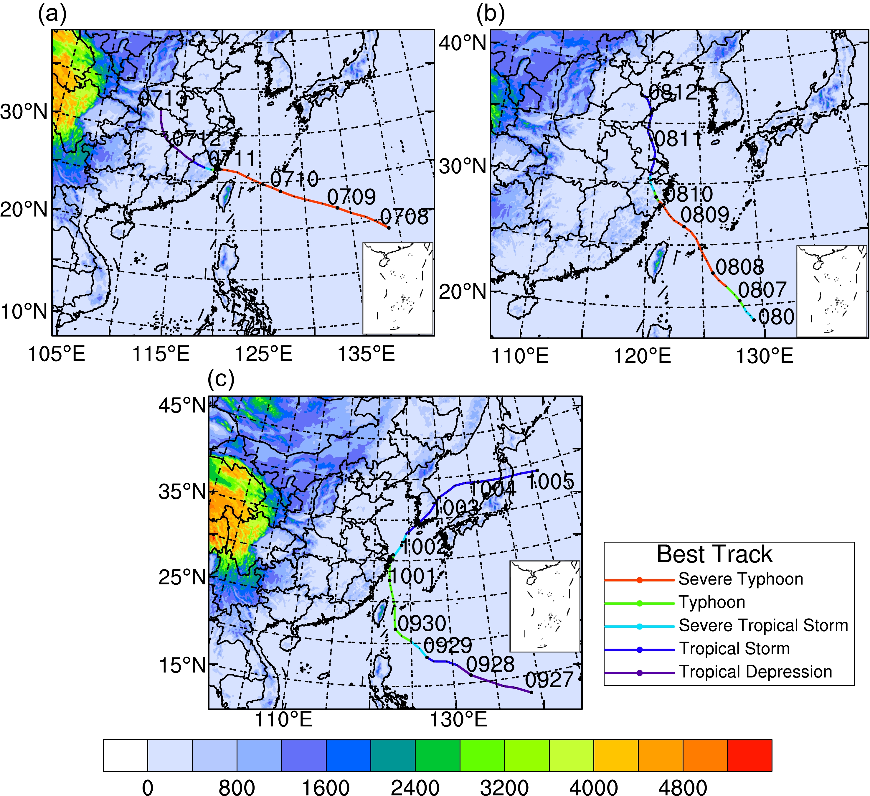
In this study, three typhoons—Maria (2018), Lekima (2019), and Mitag (2019)—are chosen to investigate the impacts of assimilating the FY-4A AGRI radiances on the typhoon initialization. The three typhoons were generated after the operational run of the FY-4A satellite and had destructive effects on the southeast coastal region of China. It is interesting to evaluate the impact of FY-4A AGRI radiance DA considering the variety of the three typhoons, since their landfall locations were rather different with distinct moving directions. The observed tracks of the typhoons are shown in Fig. 1. The best-track datasets used in this study are from the China Meteorological Administration (CMA) (Ying et al., 2014).
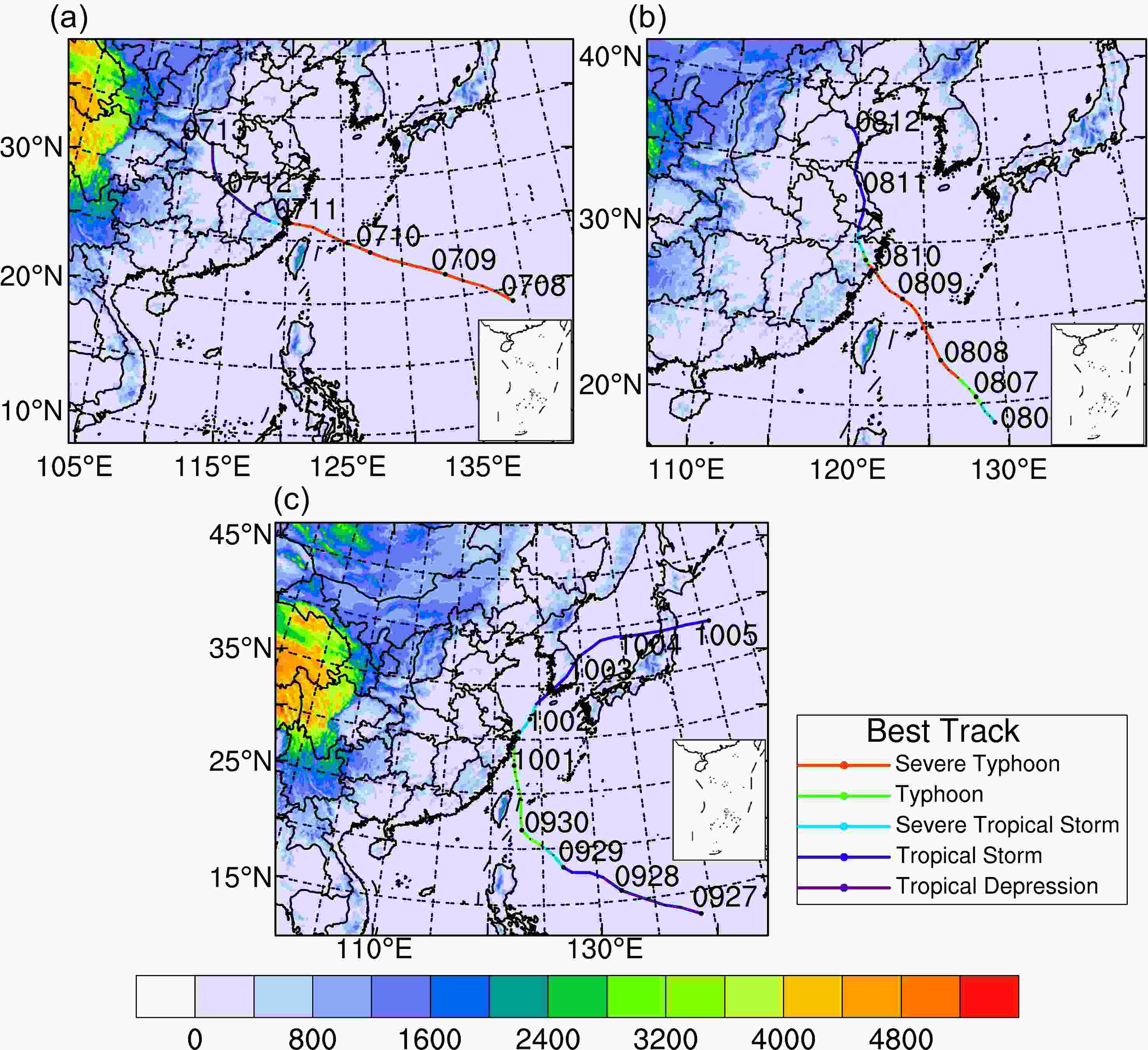
Figure 1. The tracks of Typhoon (a) Maria (2018), (b) Lekima (2019), and (c) Mitag (2019). The areas are the model domains and the filled colors are the terrain altitude (units: m).
Typhoon Maria (2018) was the eighth typhoon in 2018. After its formation, it moved northwest and intensified to a severe typhoon. At about 0000 UTC 11 July, Maria (2018) landed in Fujian, China, and was weakened sharply in the subsequent 12 h due to frictional consumption. According to official statistics, Maria (2018) caused two casualties and $628 million of economic losses (Yin et al., 2021). Typhoon Lekima (2019) was the ninth typhoon in 2019, which was the strongest typhoon to make landfall in China that year (Xu et al., 2022). It landed in Wenling, Zhejiang Province, at 1945 UTC 9 August, with a minimum sea level pressure (MSLP) of 930 hPa and brought large amounts of precipitation to eastern China. Typhoon Mitag (2019) was also a typhoon that occurred in 2019. It was the eighteenth typhoon of the year and initiated at 0000 UTC 28 September. Although it did not cause long-lasting landfall, heavy precipitation occurred in Zhejiang Province.
-
AGRI has 14 spectral bands from visible (0.47 μm) to longwave infrared (13.5 μm) wavelength (Zhang et al., 2018), compared to its predecessor, the FY-2 series satellites, with five infrared bands. Channels 1–6 are visible and near-infrared bands, mainly detecting information on the reflection and scattering of the surface and atmosphere during daytime. Channels 7–8 are mid-infrared bands, which can detect information from the sun, the earth, and clouds. Channels 9–10 are the vapor-absorptive bands, which can reflect the moisture information in the middle and upper atmosphere, while channel 14 is the CO2 absorption band. Channels 11–13 are the atmospheric window channels with low atmospheric absorptivity. The differences in the radiance observations and the simulated radiance from the background with the RTTOV (the observed minus the simulated radiance) are applied to estimate the observation error statistitically for roughly one week every 6 h.
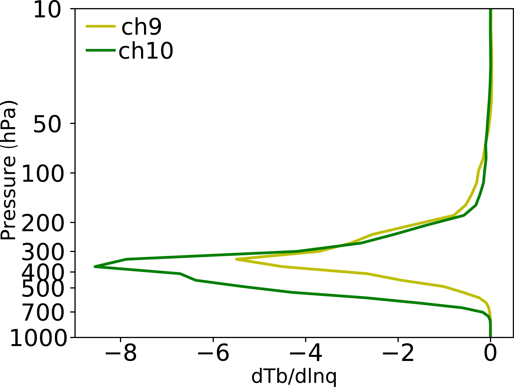
Figure 2 shows the Jacobian functions of the water vapor channels 9 and 10 using the clear-sky atmosphere in the case of Maria (2018). The Jacobian functions explain the sensitivity of the top-of-the-atmosphere radiance to changes in the atmosphere or surface. It can be found that the Jacbians of the water vapor for channel 9 and channel 10 are generally large at higher levels around 300 hPa and 400 hPa, respectively. In this study, the two water vapor absorption channels are assimilated since it has previously been shown that water vapor channels can provide accurate moisture information (Xu et al., 2021).
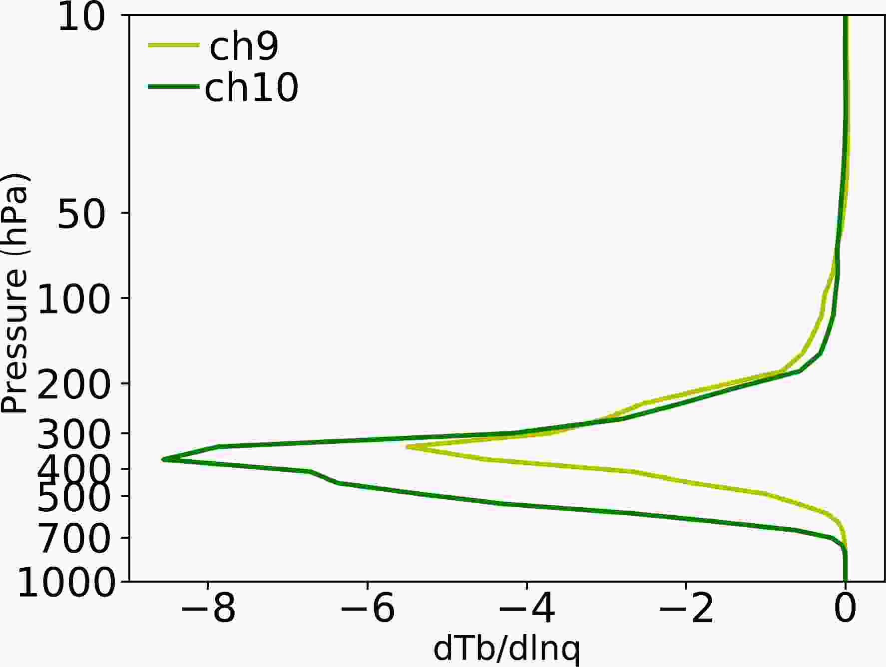
Figure 2. Jacobian of the specific humidity of channel 9 and channel 10.
-
In this study, version 4.3 of the WRF model (Skamarock et al., 2021) is used. The domains for each typhoon case are illustrated in Fig. 1 and their detailed domain settings are listed in Table 1. The initial values and boundary conditions are provided by 0.25° × 0.25° NCEP GFS analysis data. The physics parameterization schemes used in the experiments include the WDM6 microphysics scheme (Lim and Hong, 2010), the Grell–Freitas cumulus scheme (Grell and Freitas, 2014), the YSU boundary layer scheme (Hong et al., 2006), the Dudhia scheme (Dudhia, 1989), and the RRTM scheme (Mlawer et al., 1997) for shortwave and longwave radiation.
Typhoon Model center Horizontal grid (spacing) (lat×lon) Vertical levels (pressure top) Maria (2018) (25°N, 123°E) 501×401 (9 km) 57 (10 hPa) Lekima (2019) (30°N, 123°E) 381×311 (9 km) 57 (10 hPa) Mitag (2019) (30°N, 123°E) 559×469 (9 km) 57 (10 hPa) Table 1. Domain settings.
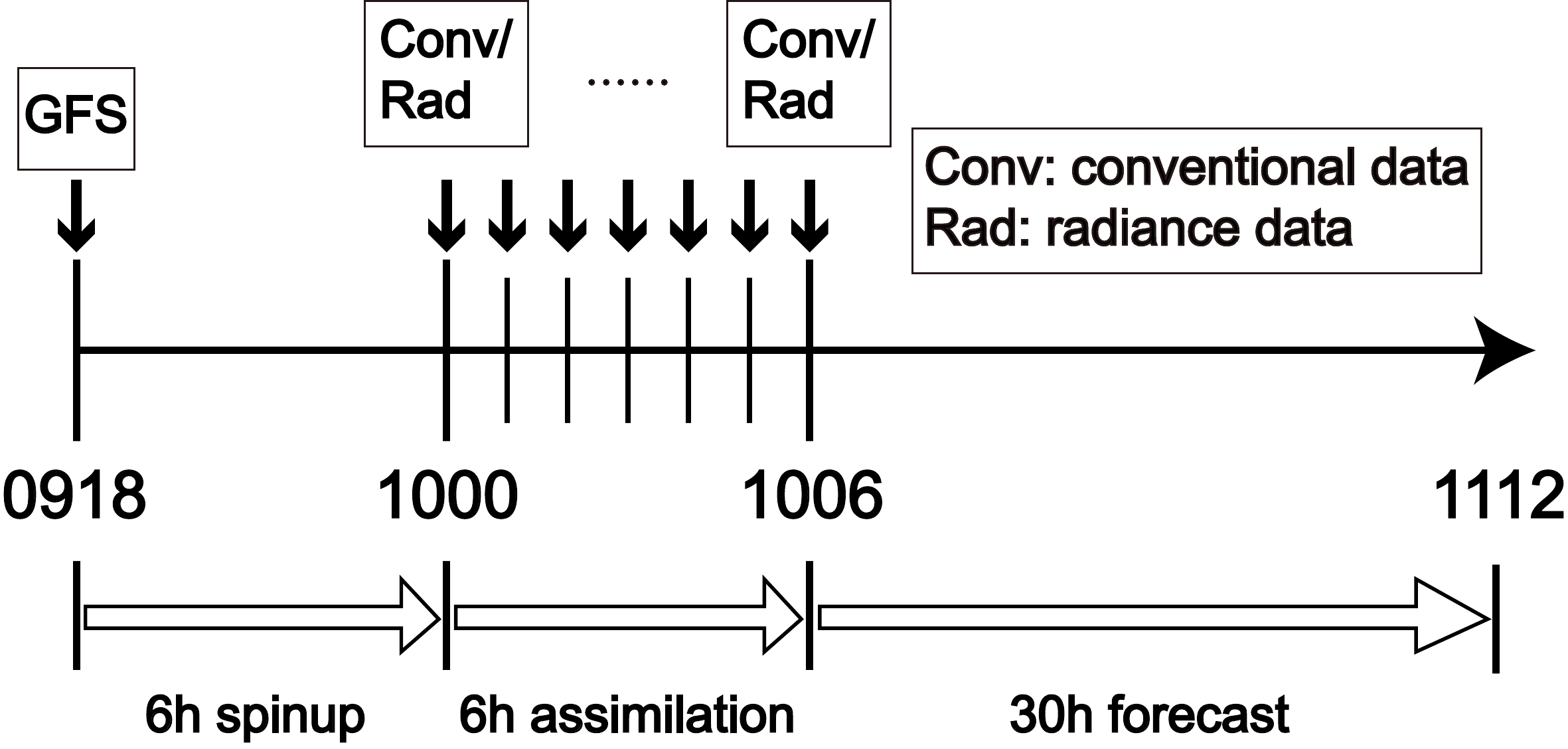
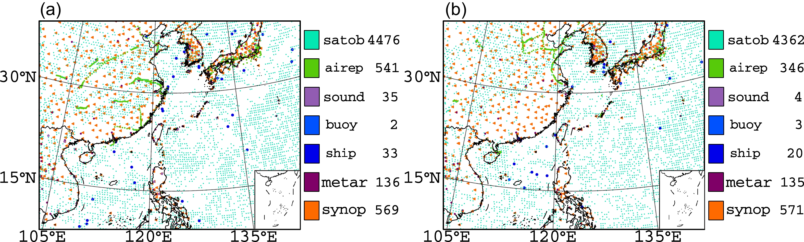
Figure 3 illustrates the experimental flow chart of the Maria (2018) case. Firstly, a 6-h forecast driven by 0.25° GFS data at 1800 UTC 9 July is used as the first guess for the first analysis cycle. In the following 6 h, six assimilation experiments are conducted with hourly intervals. The six experiments differ in their observations assimilated and cloud detection methods employed, as shown in Table 2. The distributions of global telecommunications system (GTS) data used for the Maria (2018) case in the first and the final assimilation are shown in Fig. 4 as an example. A 30-h forecast is carried out from the analysis at 0600 UTC 10 July for each experiment. In order to avoid correlations between adjacent pixels, a thinning mesh with six times the horizontal distance is applied. Similar to the Maria (2018) case, the differences of the Lekima (2019) and Mitag (2019) cases in their experimental setup is their start times and forecast durations. The analysis starts at 1200 UTC 8 August 2019 and a 30-h forecast is performed for Lekima (2019), while the Mitag (2019) case begins the analysis at 0600 UTC 30 September 2019 followed by a 48-h forecast after the DA cycles.
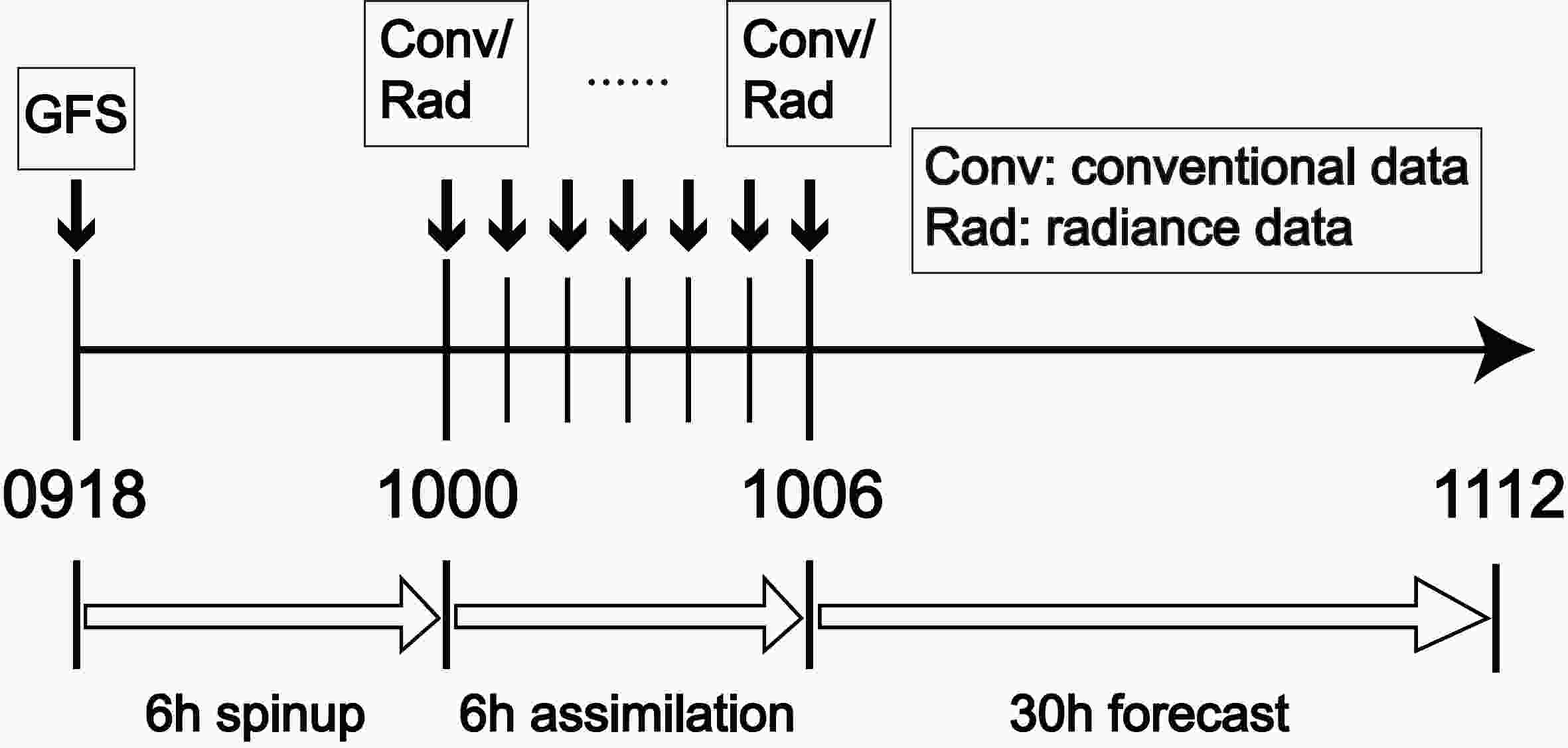
Figure 3. Flow chart of the Maria (2018) case.
Expriment abbreviation Data employed Cloud detection CNTL GTS None PF GTS and AGRI radiances Particle filter MMR GTS and AGRI radiances Multivariate and minimum residual CLM0 GTS and AGRI radiances Reject pixels with value = 0 (cloudy) in cloud mask file CLM01 GTS and AGRI radiances Reject pixels with value ≤ 1 (cloudy and probably cloudy) in cloud mask file CLM012 GTS and AGRI radiances Reject pixels with value ≤ 2 (cloudy, probably cloudy, and probably clear) in cloud mask file Table 2. The experiments.
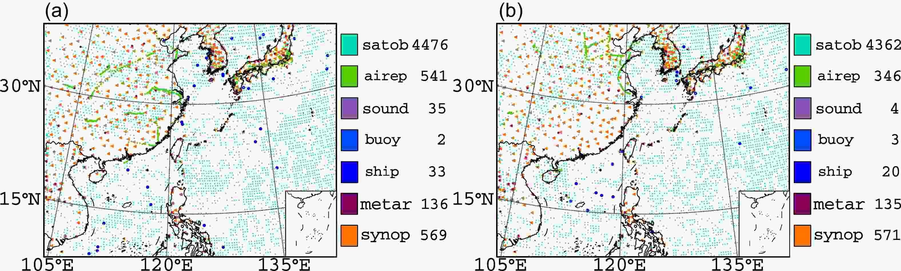
Figure 4. Distributions of GTS observations at (a) 0000 UTC and (b) 0600 UTC 10 July 2018.
-
In this section, the track and MSLP forecast of Maria (2018) is first presented, followed by detailed analyses and diagnoses of Maria (2018). Lastly, the track and intensity forecasts of Lekima (2019) and Mitag (2019) are shown.
-
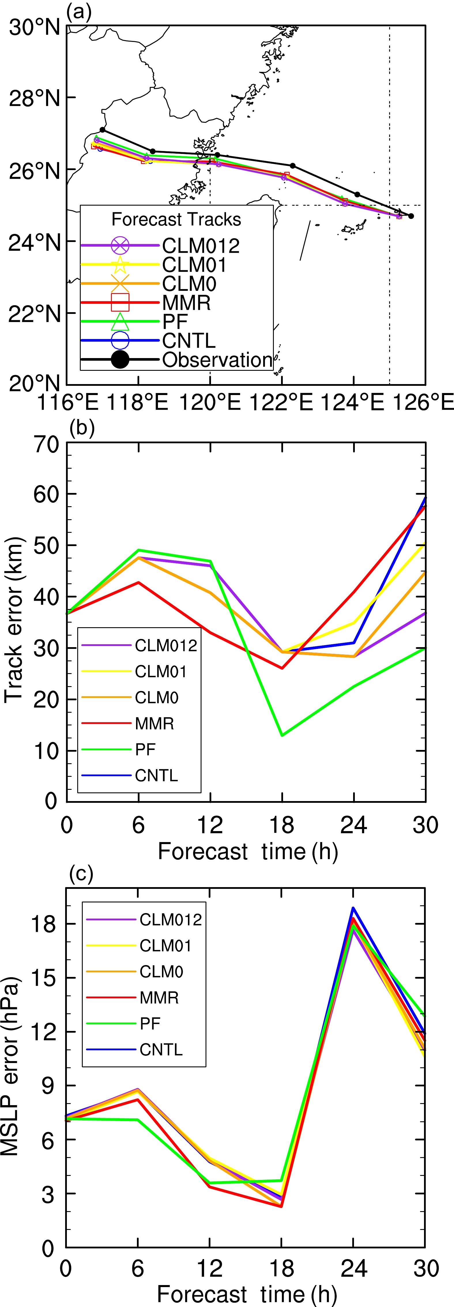
Figure 5 shows the forecast results of all experiments. For the track forecast (Fig. 5a), the differences of all experiments are not evident for the first 12 h. Owing to the weakened northeast pressure gradient, the track of the PF experiment moves more northward, leading to reduced track errors for later hours. This can be shown by the quantitative track error in Fig. 5b. In the first 12 h, the track error of the MMR experiment is the smallest, while the errors of other experiments are comparable. The error of the MMR experiment undergoes a rapid increase in the final 12 h, while the track error of the PF experiment decreases in the final 18 h. For the intensity forecast (Fig. 5c), the PF experiment is superior in the first 12 h, while the intensity errors of all experiments are similar in the remaining time.
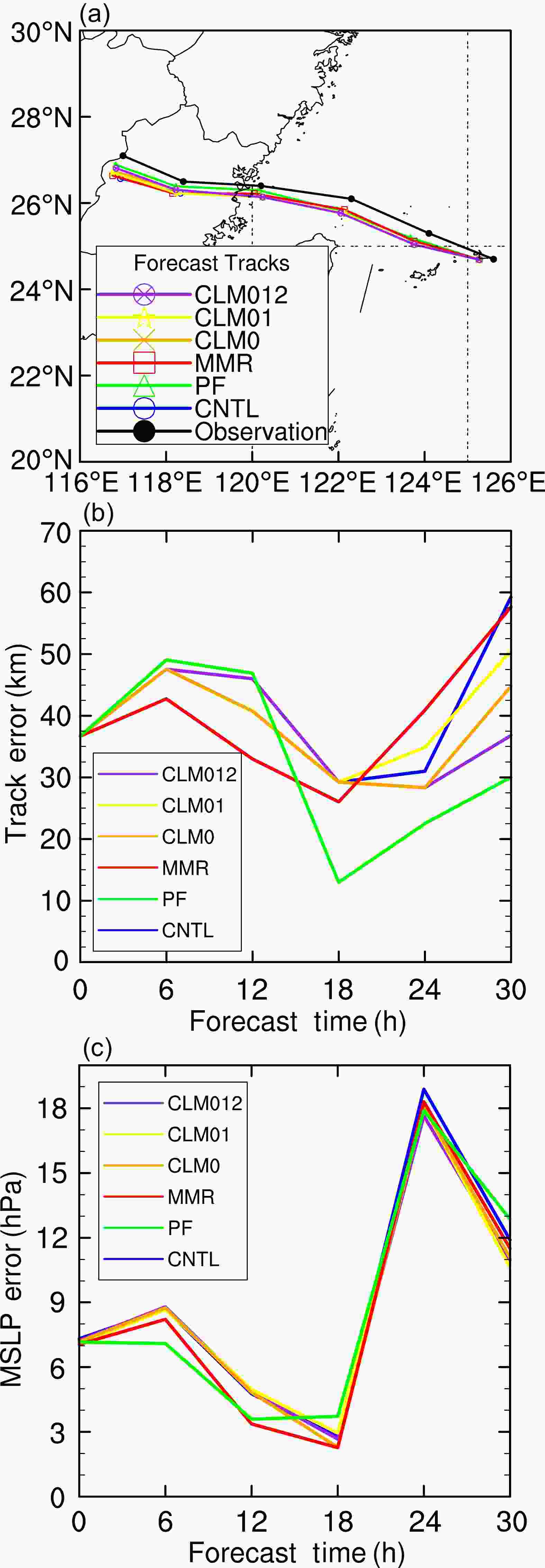
Figure 5. The (a) track forecast, (b) track error (units: km), and (c) MSLP error (units: hPa) of Maria (2018).
-
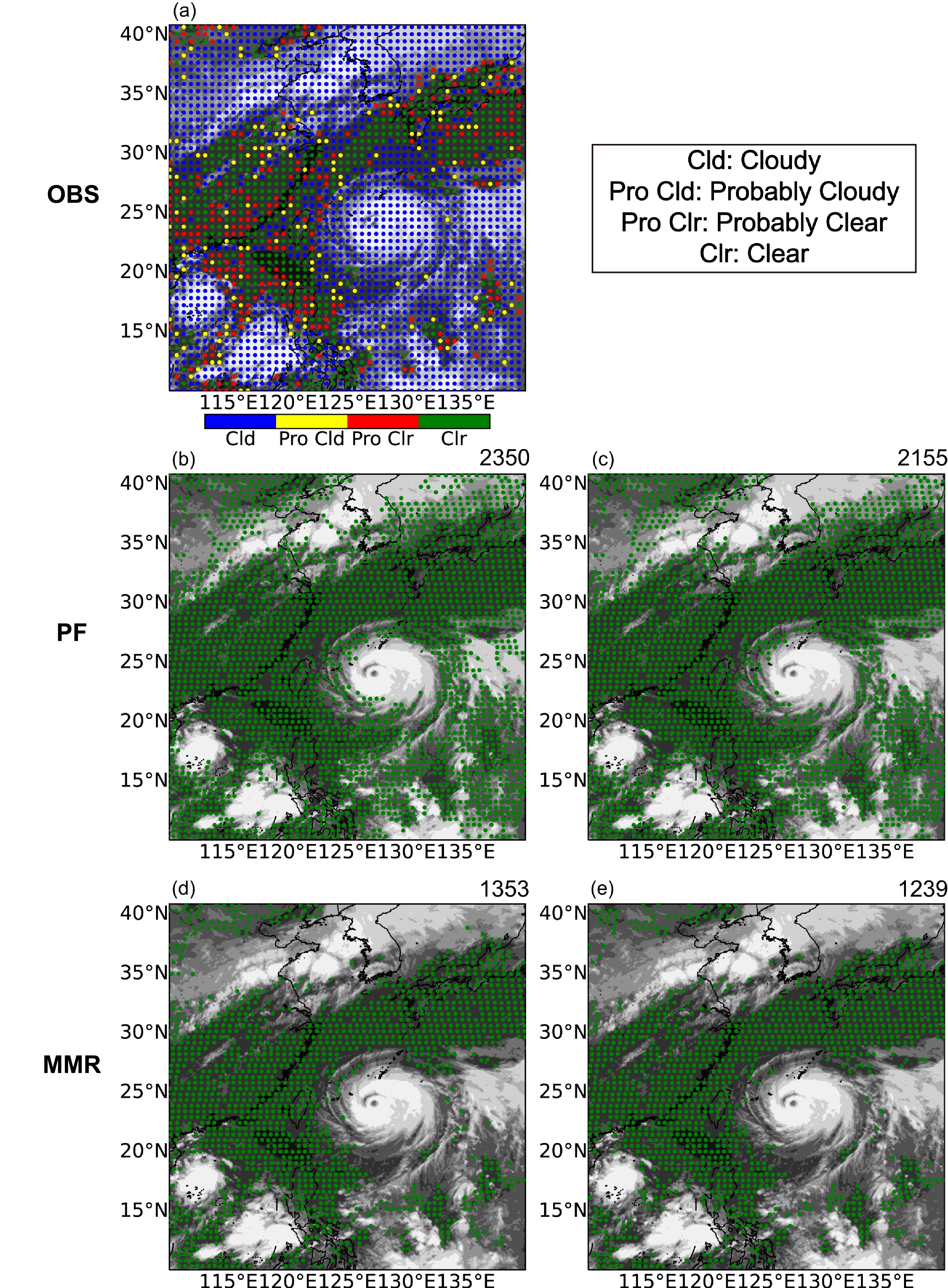
Figure 6a shows the cloud mask information from the FY-4A product, while Figs. 6b–e display the reserved pixels with different cloud detection schemes. The numbers of reserved pixels are marked in the top-right corner in each figure panel. In Fig. 6a, the pixels over the spiral cloud system of Typhoon Maria (2018) and tropical convective clouds are recognized as cloudy. At the edges of these regions, pixels are mainly viewed as probably cloudy or probably clear, while pixels away from these regions are mainly determined as clear. By comparing the PF scheme and the MMR scheme with the same channel (Fig. 6b versus Fig. 6d or Fig. 6c versus Fig. 6e), it can be found that the number of reserved pixels in the PF scheme is overall larger than that in the MMR scheme (2155 versus 1239 for channel 10), especially in the northeast of the typhoon. This is consistent with the cloud height retetrievals from the PF and MMR methods in Xu et al. (2016). In addition, as expected, for the same cloud detection scheme, the number of pixels of channel 9 is larger than that of channel 10, consistent with the higher peaking Jacobian of channel 9 in Fig. 1 with a higher possibility of being free from the contamination of clouds. Overall, the PF scheme reserves the most pixels, while the scheme using cloud masks from the FY-4A product keeps the least pixels.
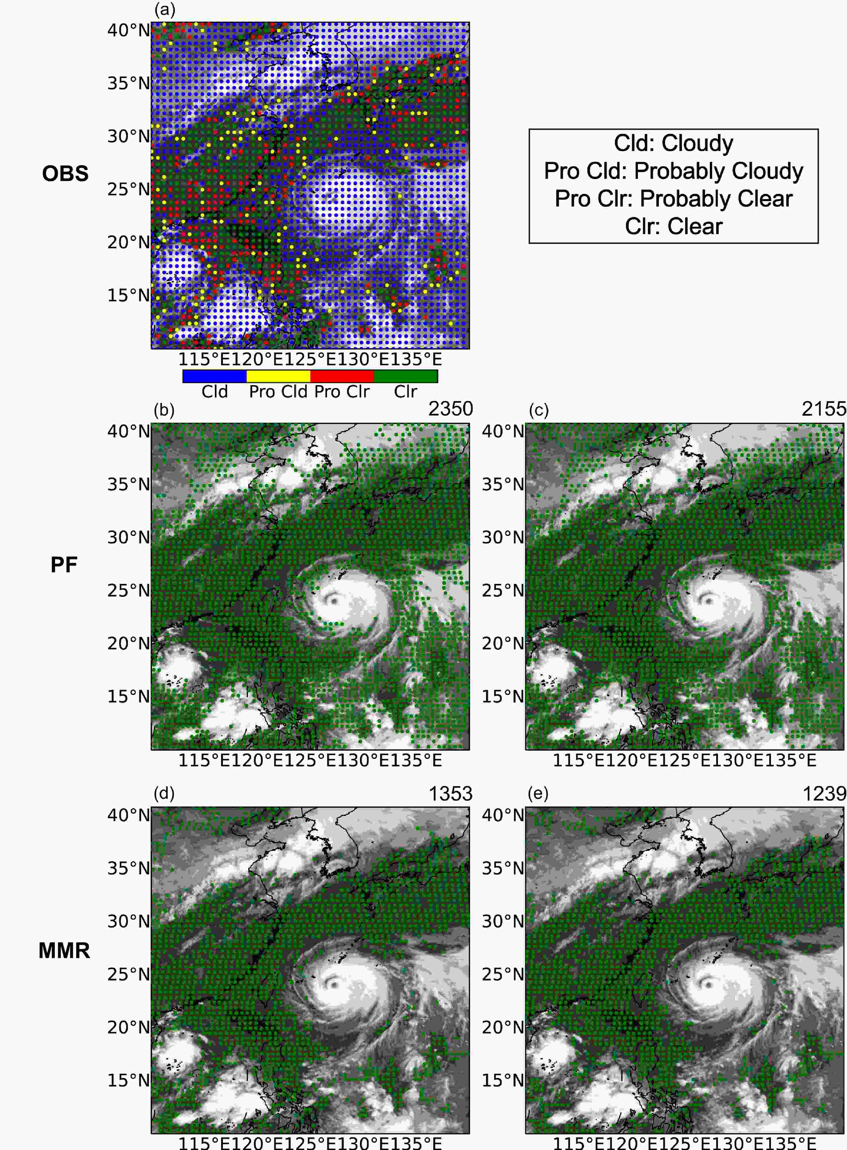
Figure 6. The (a) cloud mask product, (b, c) used pixels of (b) channel 9 and (c) channel 10 with the PF cloud detection scheme, and (d, e) used pixels of (d) channel 9 and (e) channel 10 with the MMR cloud detection scheme, at 0000 UTC 10 July 2018. The number of reserved pixels is marked in the top-right corner of each panel.
-
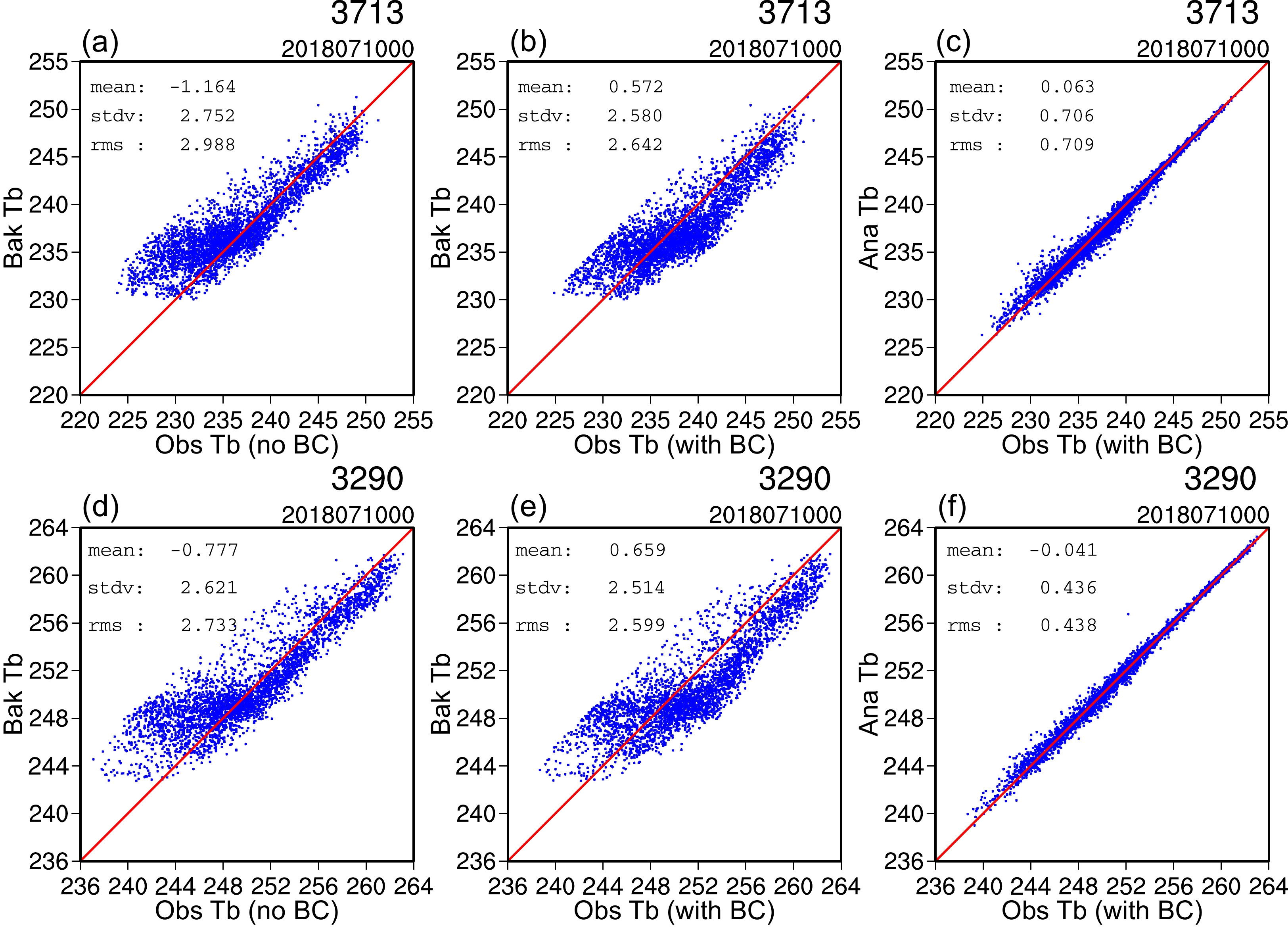
Figure 7 shows the brightness temperature scatterplots of channel 9 and channel 10 with the PF scheme at the first analysis time. Before bias correction (Figs. 7a and d), the brightness temperature simulated by the background field is higher than the observation for most cases. After bias correction (Figs. 7b and e), the relatively higher brightness temperature simulated by the background field is partially corrected. After the analysis (Figs. 7c and f), dots converge more to the diagonal with a smaller dispersion. Evidently, the mean, standard deviation, and root-mean-square values are decreased dramatically. Generally, the brightness temperature simulated by the analysis field matches well with the observations.
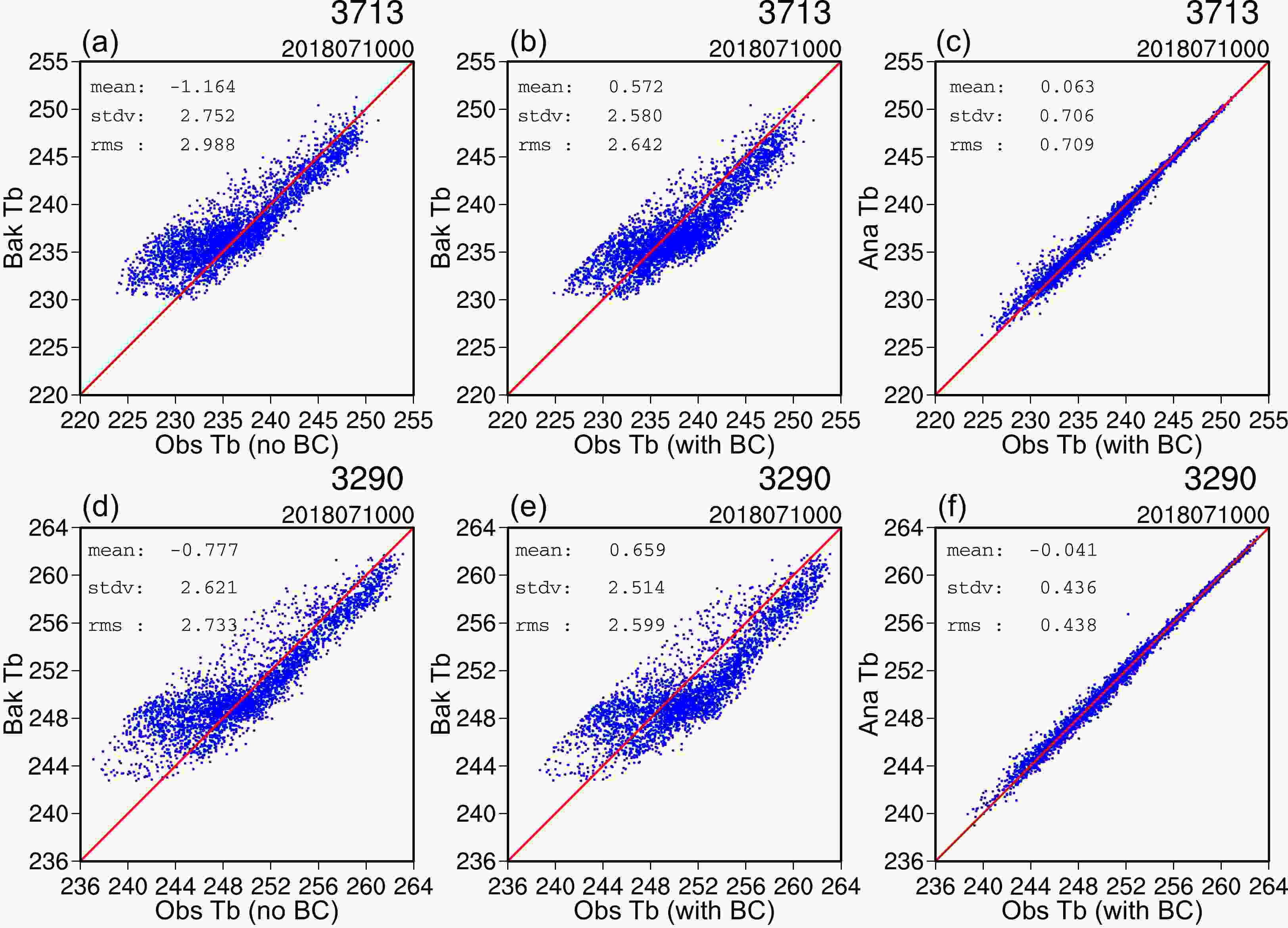
Figure 7. Brightness temperature scatterplots of the background versus observations before bias correction for (a) channel 9 and (d) channel 10; the background versus observations after bias correction for (b) channel 9 and (e) channel 10; and the analysis versus observations after bias correction for (c) channel 9 and (f) channel 10, valid at 0000 UTC 10 July 2018.
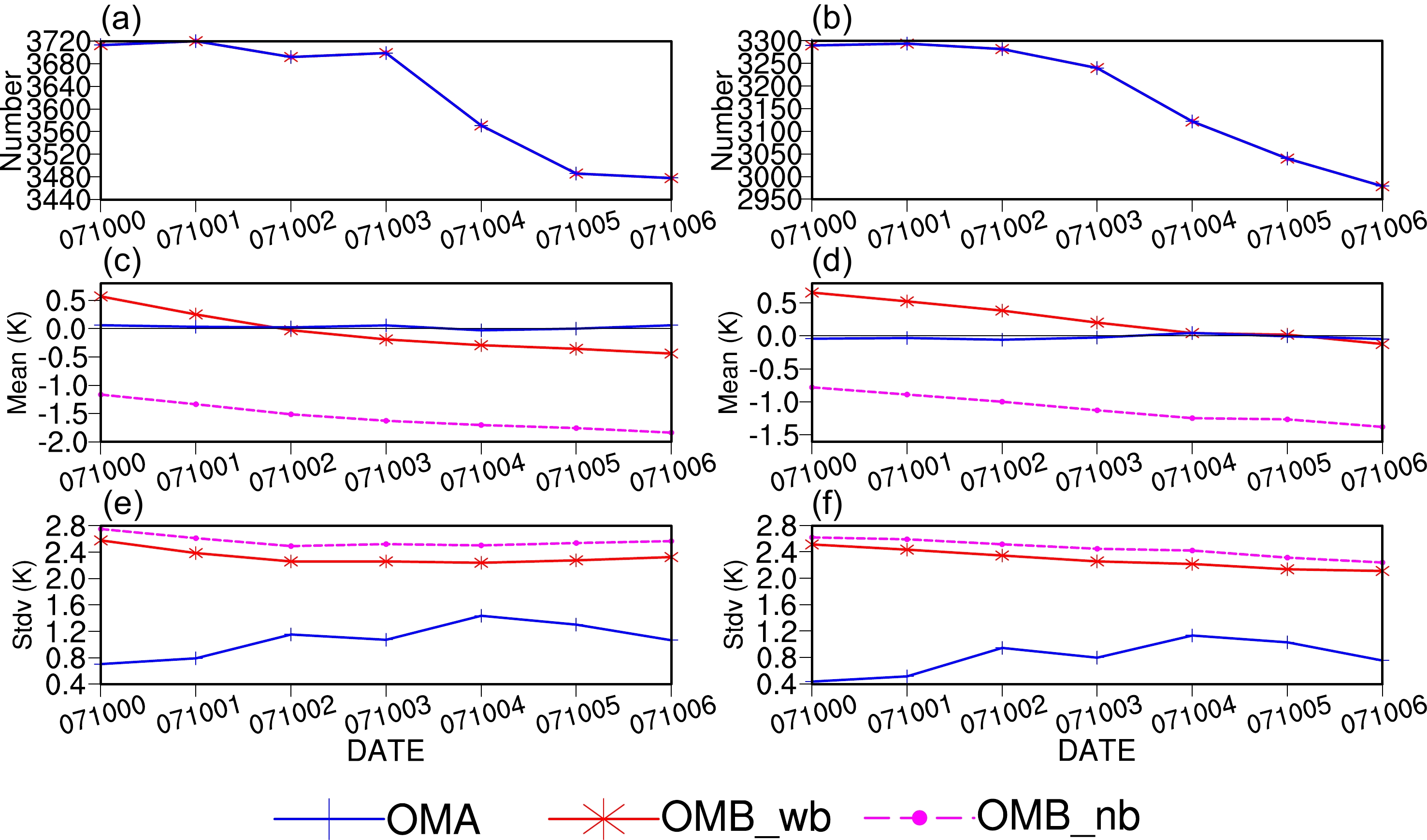
Figure 8 shows the time series of the hourly brightness temperature deviation of observation minus background (OMB) and observation minus analysis (OMA) with the PF scheme from 0000 UTC 10 July to 0600 UTC 10 July. It can be seen that the number of reserved pixels of channel 9 is larger than that of channel 10. In addition, the number of pixels for both channels reduces after 5 cycles. Before bias correction, channel 9 has greater cold biases than channel 10. After bias correction, the biases are systematically reduced with an overall same magnitude for both channels. After bias correction, both the mean and standard deviation of OMB are systematically reduced. After the analysis, the mean of OMA approaches 0 and the standard deviation decreases sharply.
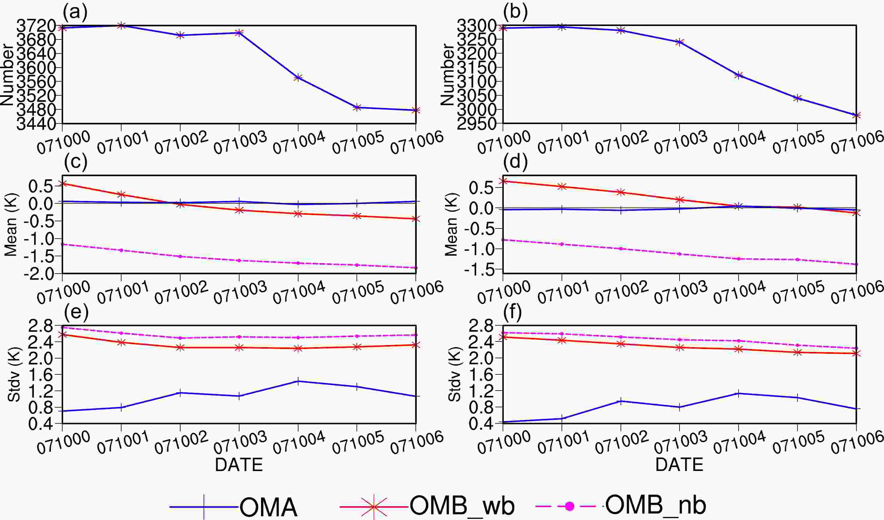
Figure 8. The reserved number of pixels for (a) channel 9 and (b) channel 10; the mean value of OMB for (c) channel 9 and (d) channel 10; and the standard deviation value for (e) channel 9 and (f) channel 10 in different analysis cycles. The blue line is the OMA, the red line is the OMB with bias correction, and the purple line is the OMB without bias correction.
-
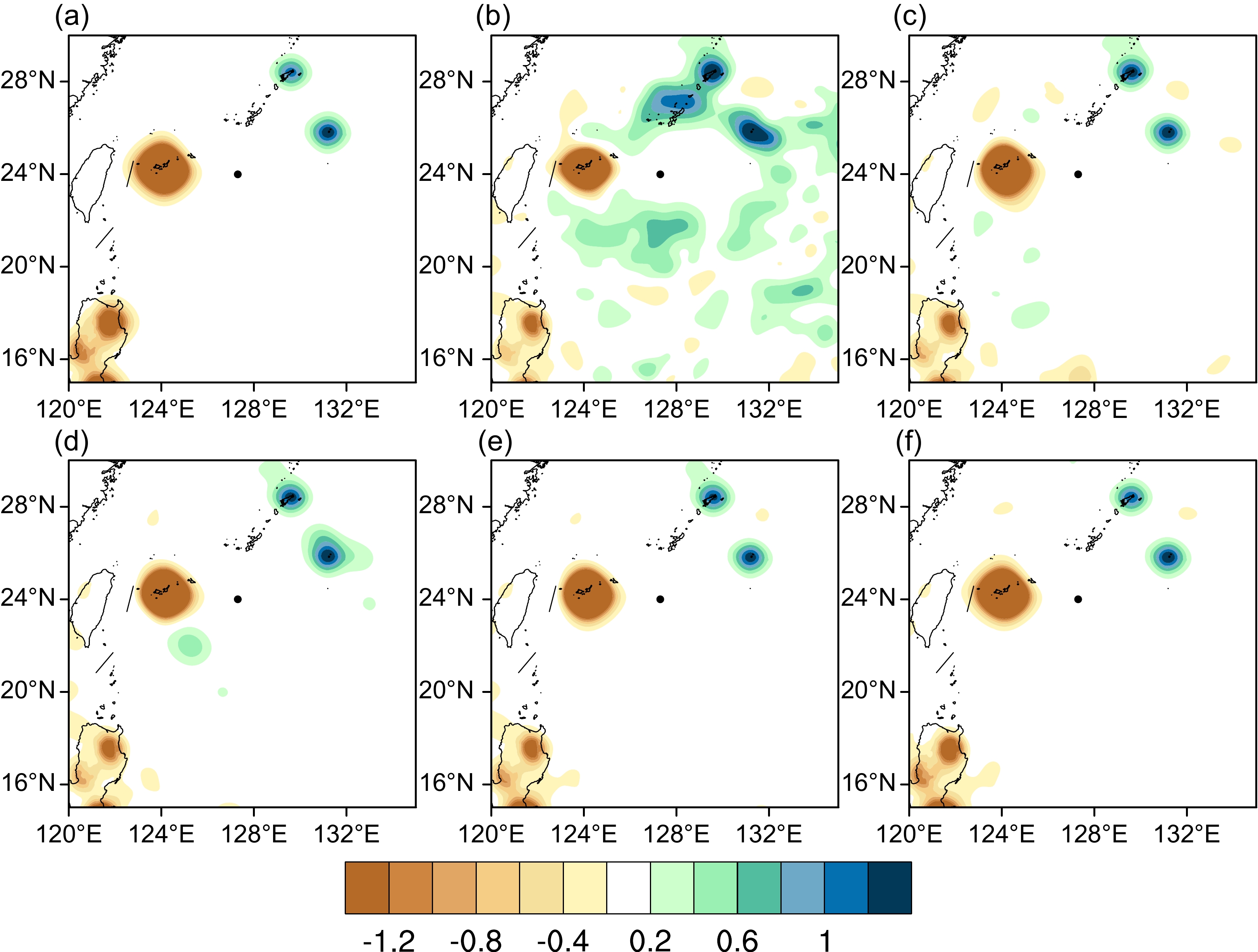
Figure 9 shows the 500-hPa geopotential height increments of all experiments at 0000 UTC 10 July 2018, describing the effects of DA on the upper trough. In the CNTL experiment (Fig. 9a), there is a positive increment to the northeast of the typhoon and a negative increment to the southwest of the typhoon. Under the influence of the pressure gradient, the track of the typhoon in the CNTL experiment tends to be southward. By comparing the two experiments with different channel-sensitive cloud detection schemes (Figs. 9b and c), the pressure gradient near the typhoon in the PF experiment is weakened, while that in the MMR experiment is strengthened. This likely explains the more northward track in the PF experiment than in the MMR experiment in the above forecast. Besides, it is found that the more data are employed, the more obvious the observed geopotential height increment is to the northeast of the typhoon via applying the cloud mask information to different extents (Figs. 9d–f). However, their increment magnitudes are consistently larger than in the PF experiment.
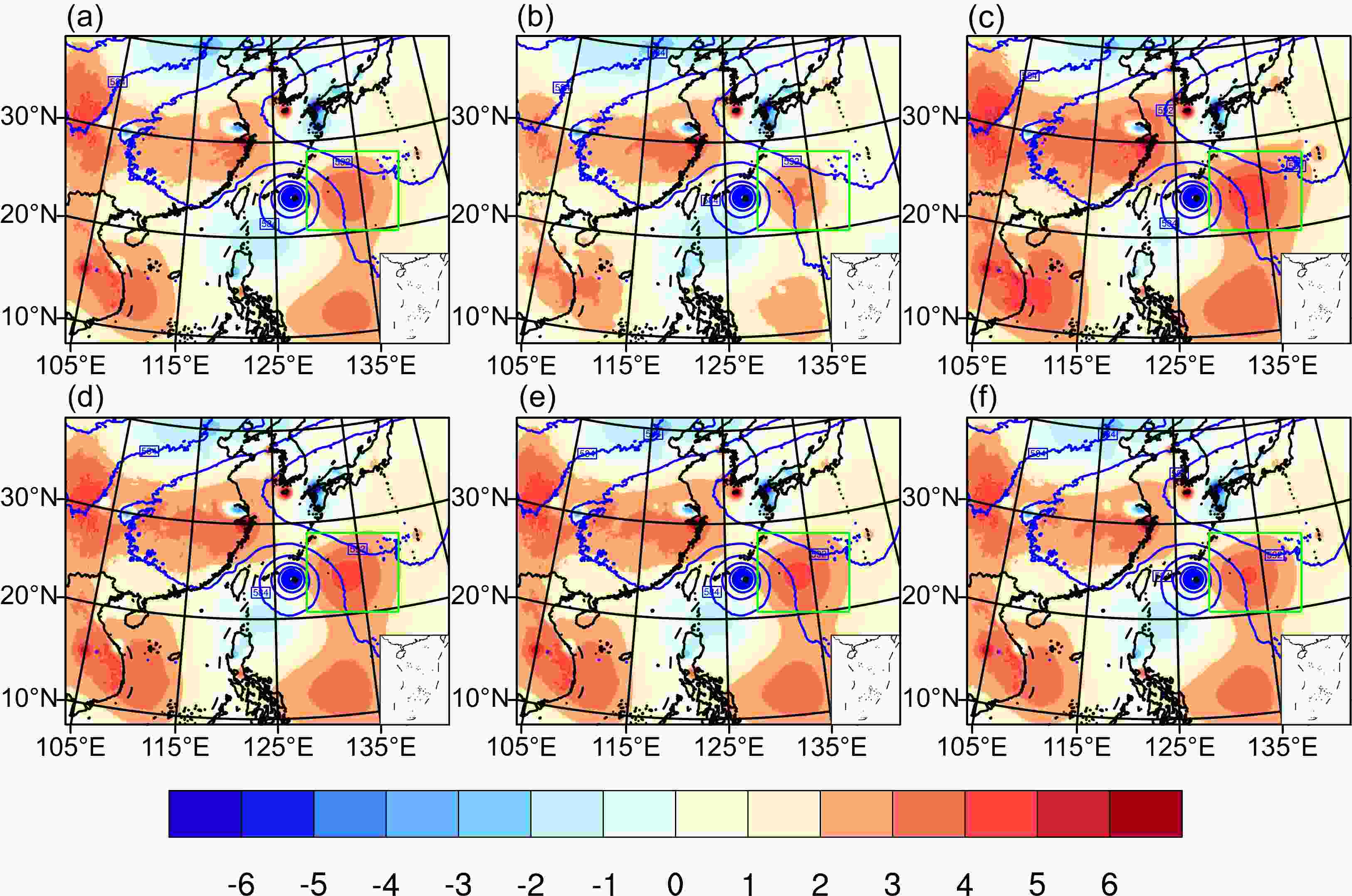
Figure 9. The 500-hPa geopotential height field (units: dagpm) and geopotential height increment (units: gpm) of the (a) CNTL, (b) PF, (c) MMR, (d) CLM0, (e) CLM01, and (f) CLM012 experiments at 0000 UTC 10 July 2018. The blue contours are the geopotential height fields, the green rectangle highlights the differences in geopotential increments, the filled colors are the increment fields, and the black dot represents the location of the typhoon center.
-
Figure 10 shows the 850-hPa temperature increments of all experiments at 0000 UTC 10 July 2018. In the CNTL experiment, no obvious increment is found in the typhoon center. By assimilating the AGRI radiance data, the warm-core structure becomes more apparent in most experiments, with a notable positive temperature increment in the vortex. In comparison, the positive temperature increment in the PF experiment is more obvious both near the typhoon core and to the southwest of the typhoon. Besides, the area of the cold center to the west of the typhoon is slightly reduced, with disconnected contours from −0.1 to 0.
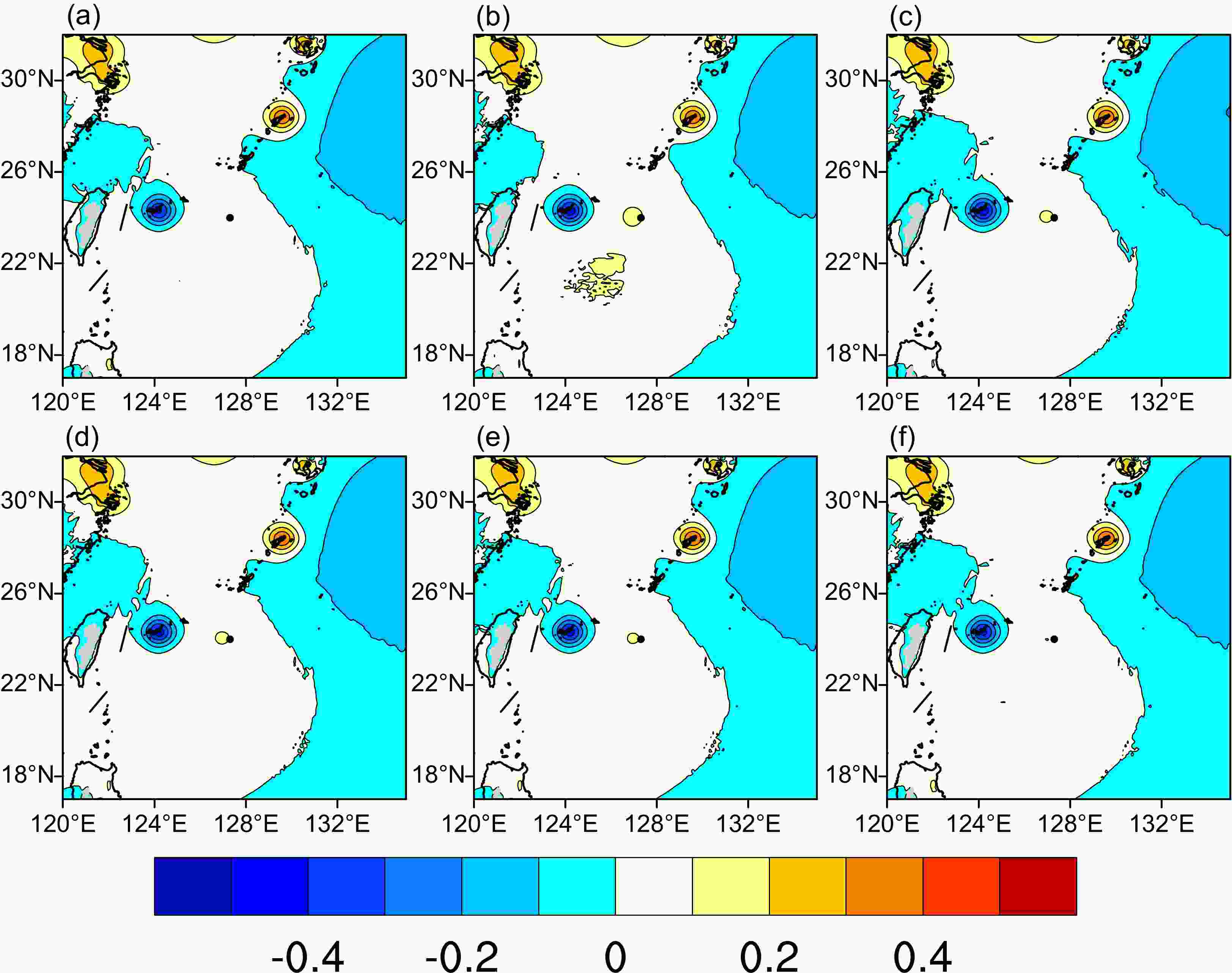
Figure 10. The 850-hPa temperature increment (units: K) of the (a) CNTL, (b) PF, (c) MMR, (d) CLM0, (e) CLM01, and (f) CLM012 experiments at 0000 UTC 10 July 2018. The black dot represents the location of the typhoon center.
-
Figure 11 shows the analysis increments of the water vapor path of all experiments at 0000 UTC 10 July 2018. In the CNTL experiment, a noticeable water vapor increment can be found in the northeast of the typhoon, accompanied by a negative increment in the west of the typhoon. In the PF experiment, the area with a positive water vapor path increment is extended to the outer side of the typhoon core. In the remaining four experiments, the magnitudes of the water vapor path increments are relatively small.
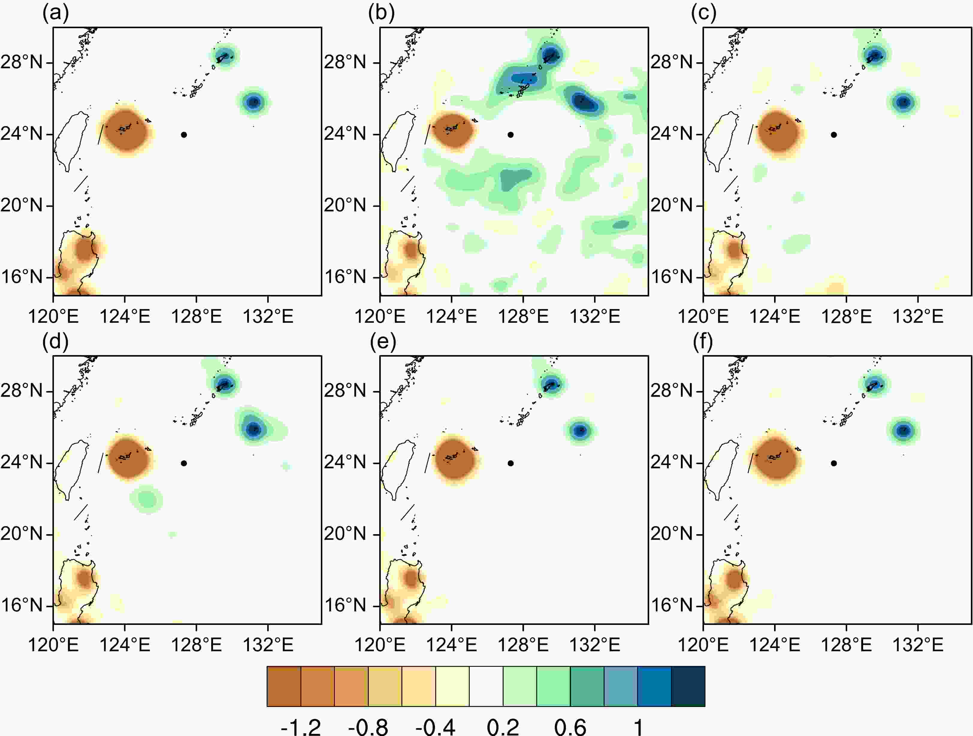
Figure 11. The water vapor path increments (units: g m−2) of the (a) CNTL, (b) PF, (c) MMR, (d) CLM0, (e) CLM01, and (f) CLM012 experiments at 0000 UTC 10 July 2018. The black dot represents the location of the typhoon center.
-
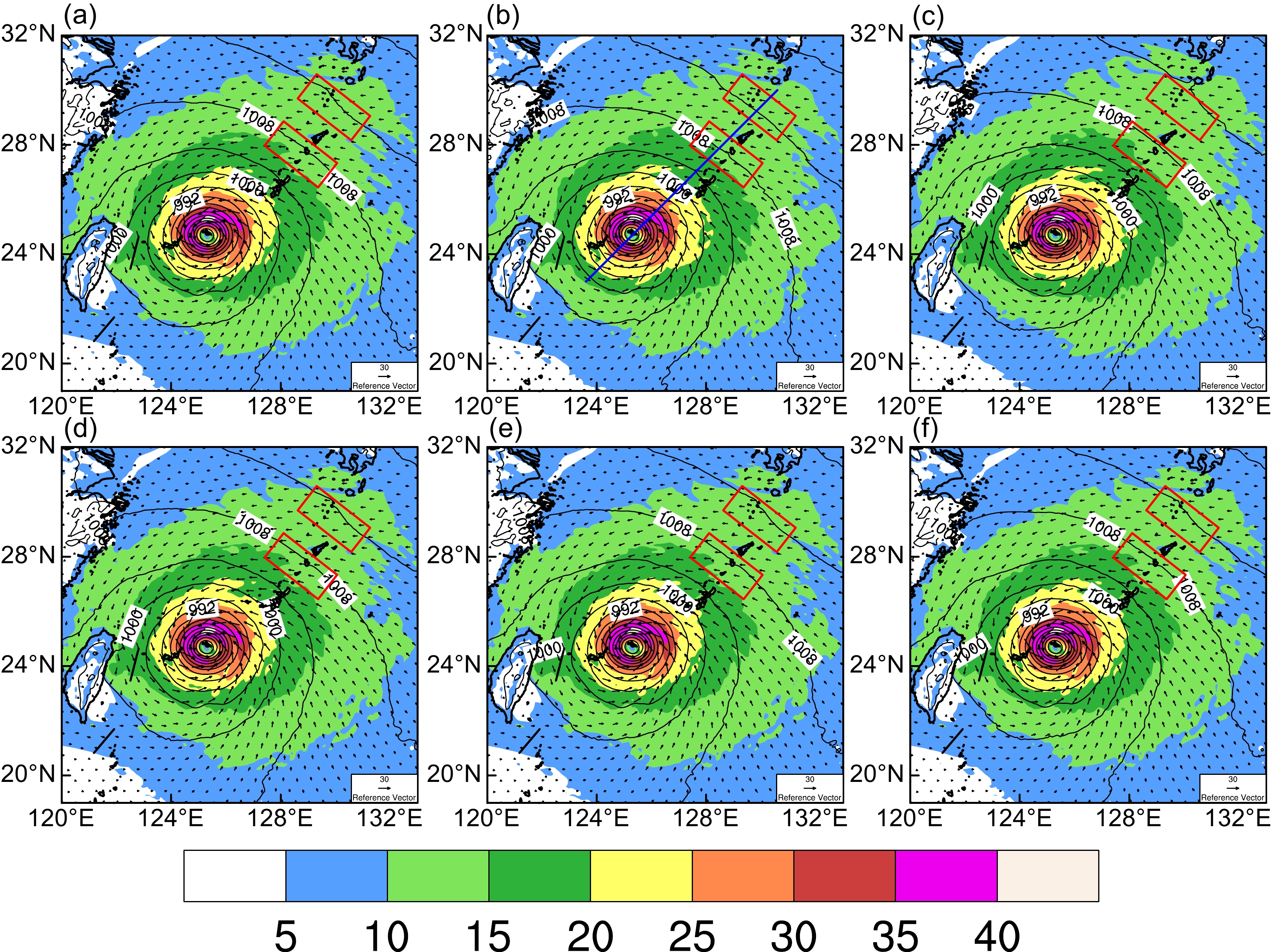
Figure 12 shows the sea-level fields of all experiments at the final analysis time. It can be seen that the 1008 and 1012 isobars marked by red rectangles in the PF experiment are contracted towards the center of the typhoon, which can strengthen the pressure gradient force in the outer side of the typhoon. According to geostrophic theory, the outside wind of the typhoon is also augmented and the area of wind speed varying from 15 to 20 m s−1 is slightly enlarged in the PF experiment. By contrast, the outside isobars are sparse in other experiments, especially in the MMR experiment. With the PF scheme, assimilating AGRI radiances yields a slightly more intensified vortex.
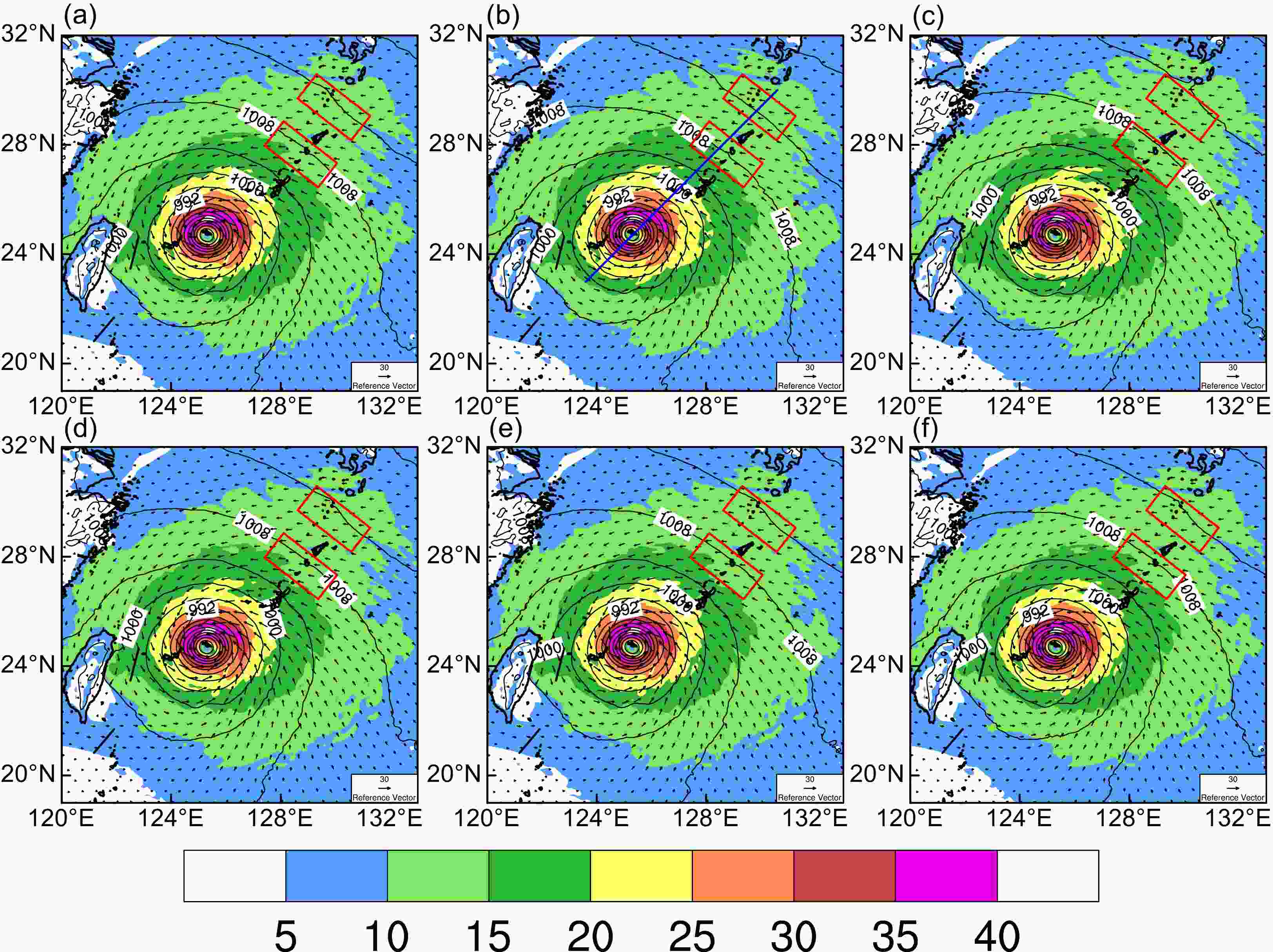
Figure 12. The sea-level fields of the (a) CNTL, (b) PF, (c) MMR, (d) CLM0, (e) CLM01, and (f) CLM012 experiments at 0600 UTC 10 July 2018. The black contours are the sea level pressure (units: hPa), the filled colors and the arrows are the wind speed (units: m s−1), the blue line is the cross-section line used in the next section, and the red rectangles are the highlighted areas.
-
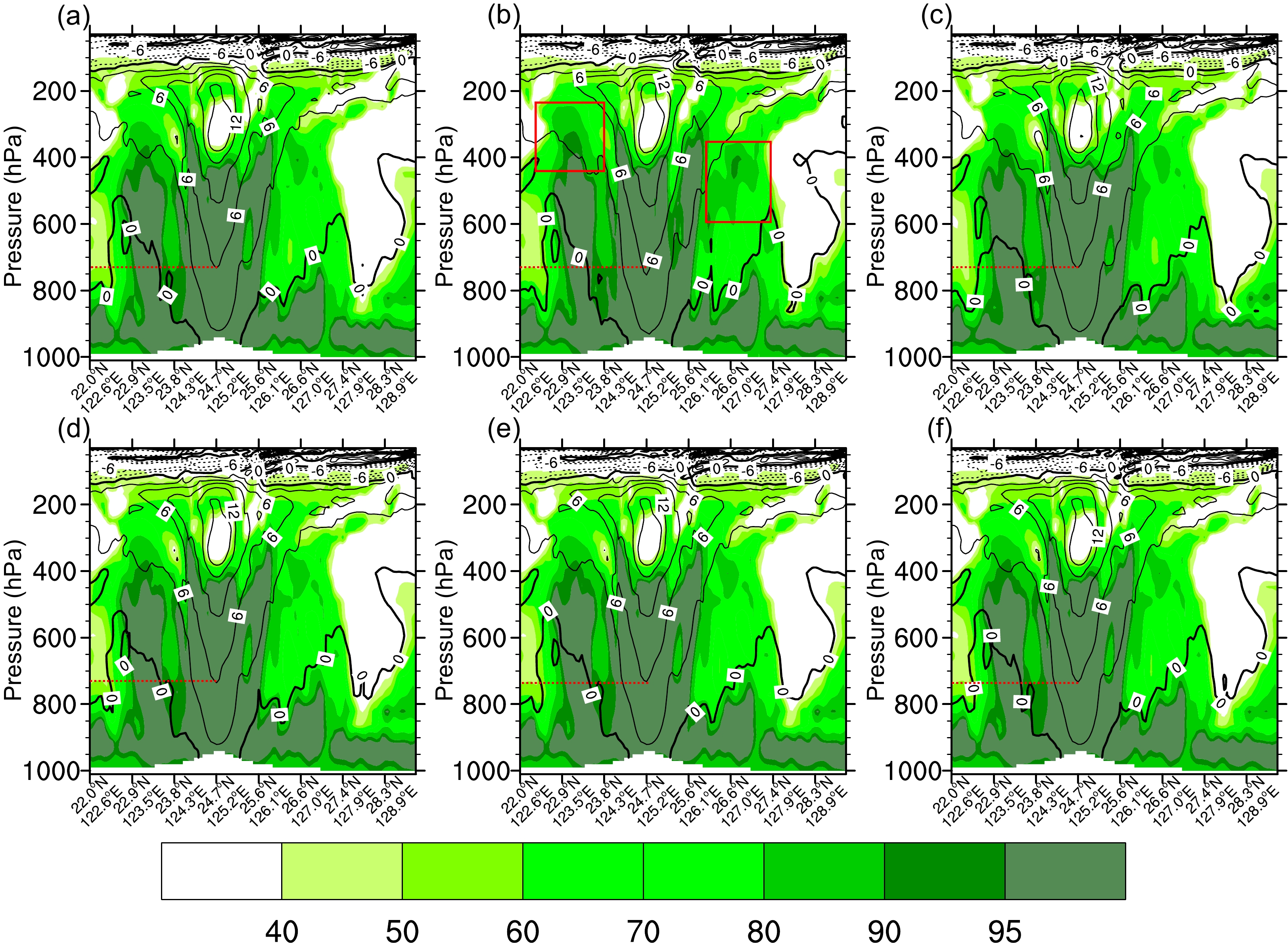
Figure 13 shows the cross section of the potential temperature anomaly and moisture field at the final analysis time. The cross-section line in Fig. 12b is used in all experiments to investigate the vertical structure across the center of the typhoon. It can be found that the lowest height of the 6-K contour is roughly at 750 hPa in the PF experiment, while that in other experiments is between 700 hPa and 750 hPa. The area of temperature anomalies with values of 15 K is expanded slightly as well in the PF experiment. Moreover, the moisture condition of the PF experiment is also favorable, with larger relative humidity observed in the southwest and northeast of the typhoon. The height of values from 80% to 90% in the southwest of the typhoon is elevated to 250 hPa (left-hand rectangle in Fig. 13b) and the originally disconnected values from 80% to 90% in the northeast of the typhoon become continuous (right-hand rectangle in Fig. 13b).
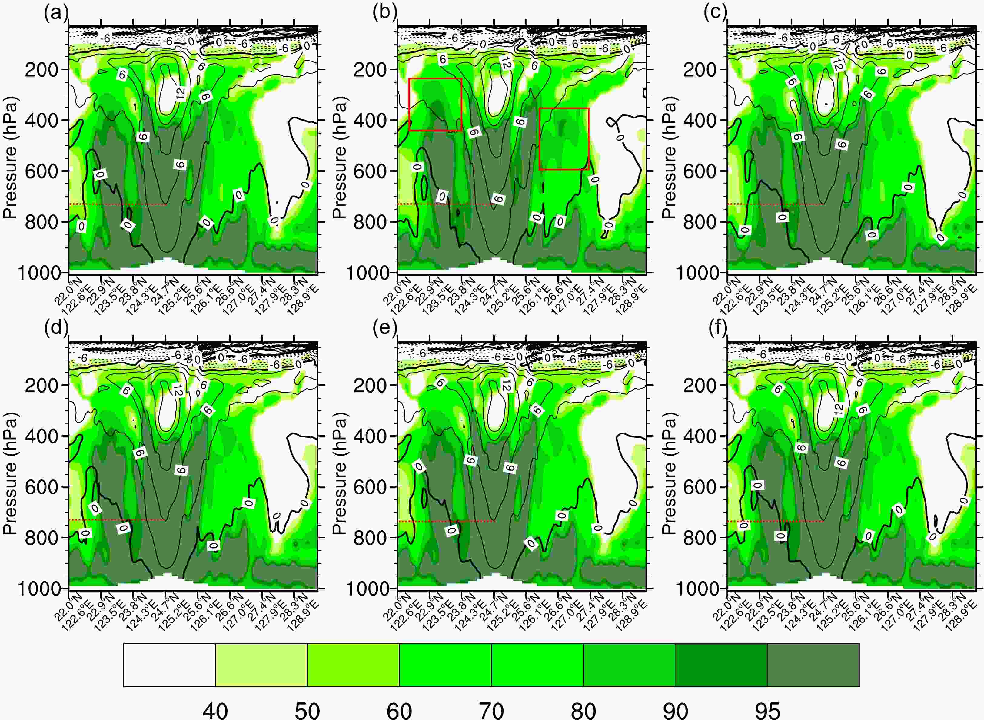
Figure 13. Cross sections of the (a) CNTL, (b) PF, (c) MMR, (d) CLM0, (e) CLM01, and (f) CLM012 experiments at 0600 UTC 10 July 2018. The black contours are the potential temperature anomaly (units: K), the filled colors are the relative humidity (%), the red dotted line is the lowest height of the 6-K contour, and the red rectangles are the moisture-rich areas.
-
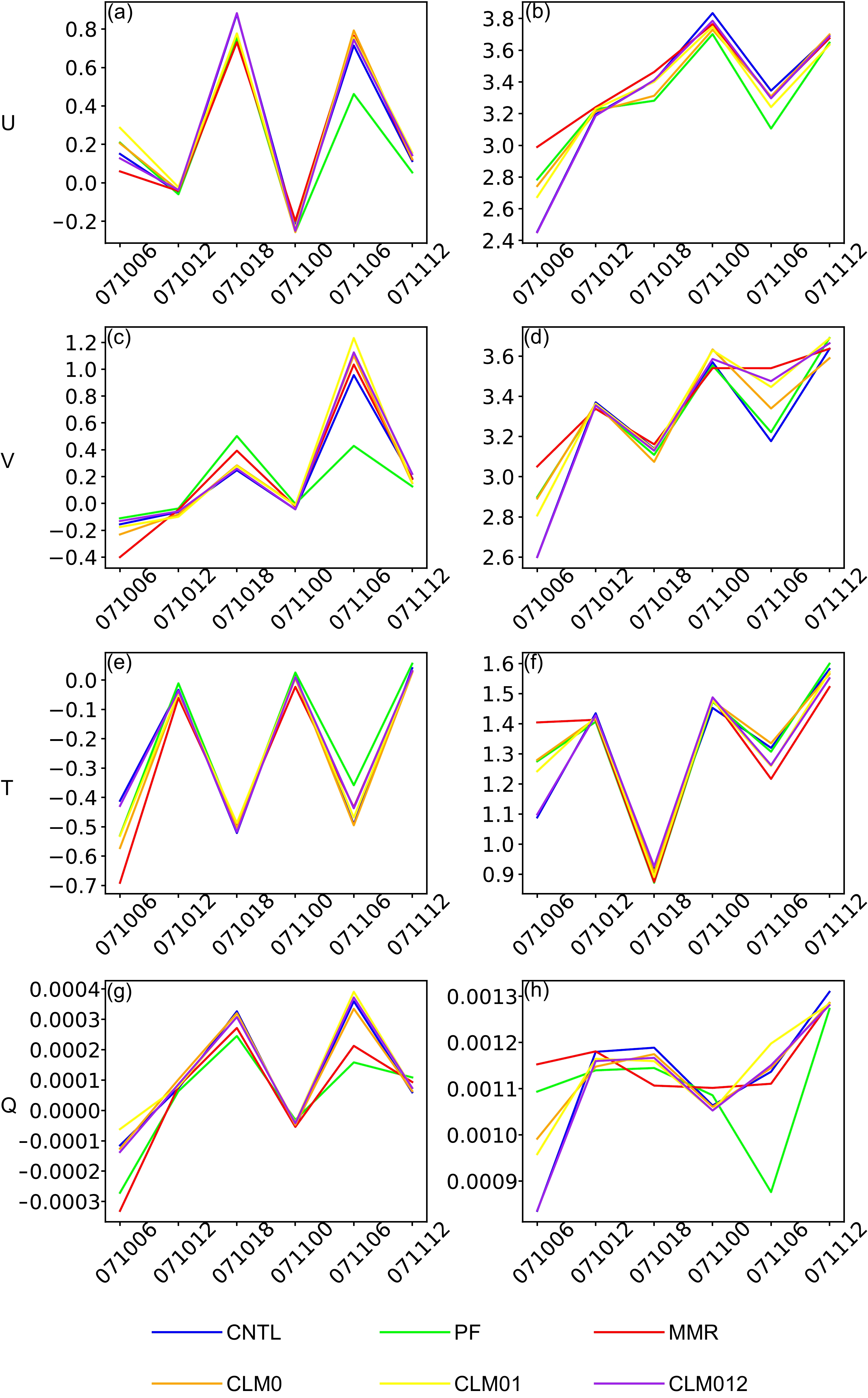
Figure 14 shows the forecast verification of u-wind, v-wind, temperature, and specific humidity against the conventional observations of soundings, with its distribution shown in Fig. 4. Overall, the PF experiment yields the smallest BIAS, especially for the last few cycles. Similarly, for the RMSE of u-wind, v-wind, and specific humidity, the PF experiment also brings some improvements, especially for the winds and humidity. It is also found that the RMSE of temperature in the MMR experiment is relatively lower than in the other three experiments that apply pixel-based cloud detection schemes.
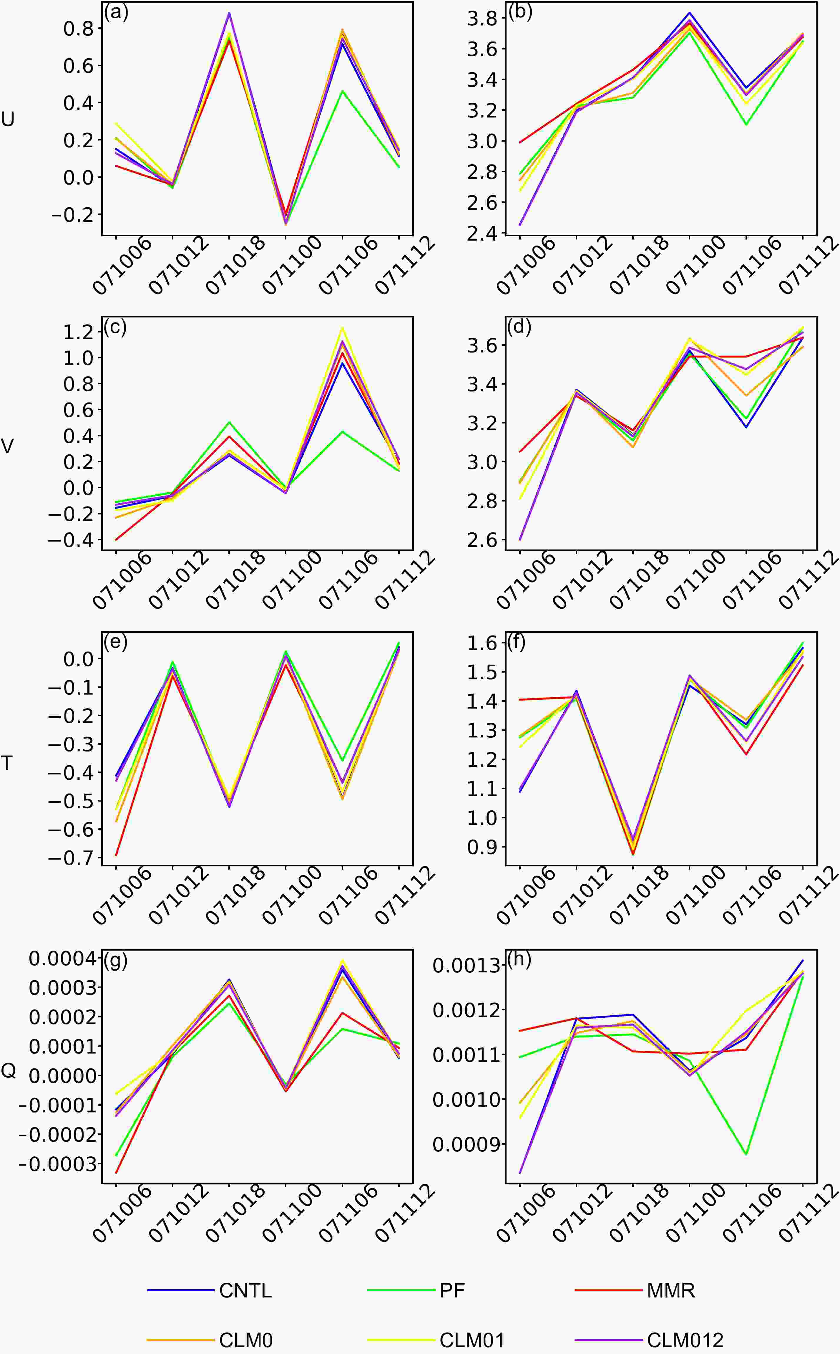
Figure 14. The (a) BIAS of U (u-wind), (b) RMSE of U, (c) BIAS of V (v-wind), (d) RMSE of V, (e) BIAS of T (temperature), (f) RMSE of T, (g) BIAS of Q (specific humidity), and (h) RMSE of Q forecast verification against the sounding observations.
For better comparison among different experiments, the averaged BIASs and RMSEs are listed in Table 3 and Table 4, respectively. It can be found that the BIAS values of the PF experiment are the closest to 0, which means no deviation, except for the Q (specific humidity) variable being slightly larger than that of the MMR experiment. As for the averaged RMSEs, apart from the T (temperature) variable, the values of the PF experiment are the smallest. To sum up, the forecast error of the model variables of the PF experiment is the smallest overall.
Bias U V T Q (10−5) CNTL 0.26 0.19 −0.23 10.88 PF 0.19 0.15 −0.22 4.57 MMR 0.24 0.19 −0.28 4.55 CLM0 0.27 0.2 −0.26 10.81 CLM01 0.29 0.23 −0.25 12.55 CLM012 0.27 0.23 −0.23 11.03 Table 3. Averaged BIASs of all experiments.
RMSE U V T Q (10−4) CNTL 3.32 3.25 1.3 11.2 PF 3.29 3.31 1.32 11.02 MMR 3.41 3.38 1.32 11.57 CLM0 3.33 3.32 1.33 11.35 CLM01 3.32 3.35 1.31 11.36 CLM012 3.3 3.3 1.29 11.08 Table 4. Averaged RMSEs of all experiments.
-
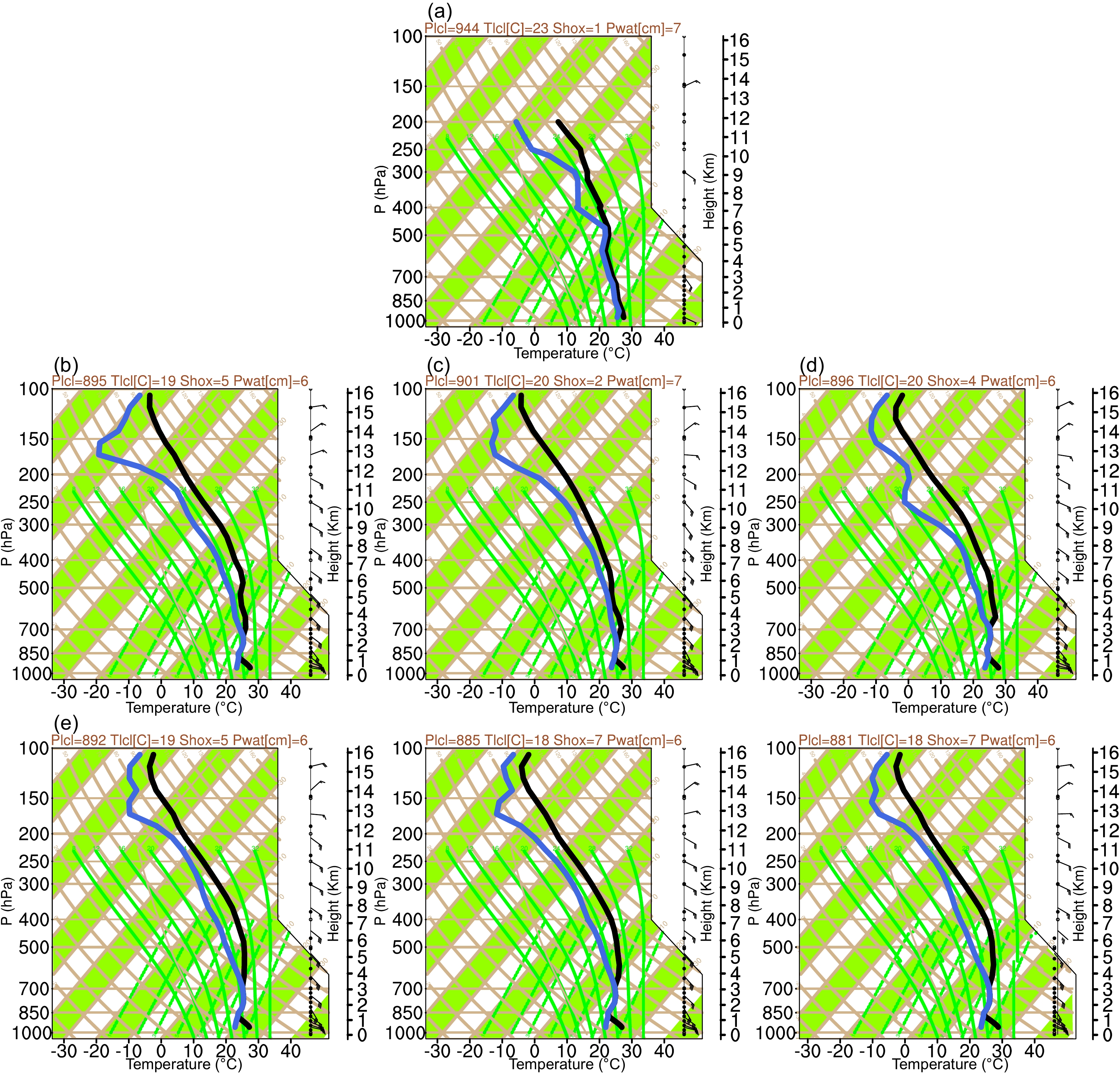
Figure 15 shows the Skew-T plots of the observation and the simulations of all experiments for the 30-h forecast valid at 1200 UTC 11 July 2018. The sounding station is in Shaowu, Fujian Province (27.33°N, 117.47°E). The simulations of the Skew-T plots are acquired by interpolation to this station from the model space. The black line is the air temperature line, and the blue line is the dewpoint temperature line. The air temperature and dewpoint temperature in the sounding observation (Fig. 15a) are almost completely overlapping below 450 hPa, indicating that the moisture condition is favorable for the occurrence of precipitation in the lower and middle layers. In all experiments, although obvious deviations can be seen compared to the observation, the air temperature and dewpoint temperature in the PF experiment are closer than in other experiments, indicating an improved water vapor condition. From the pressure of the lifting condensation level, the temperature at the lifting condensation level, the Showalter Index for stability, and the precipitable water, it seems that most of the indexes in the PF experiment match best with the observation, which are the contributors to the enhanced rainfall forecasting skill.
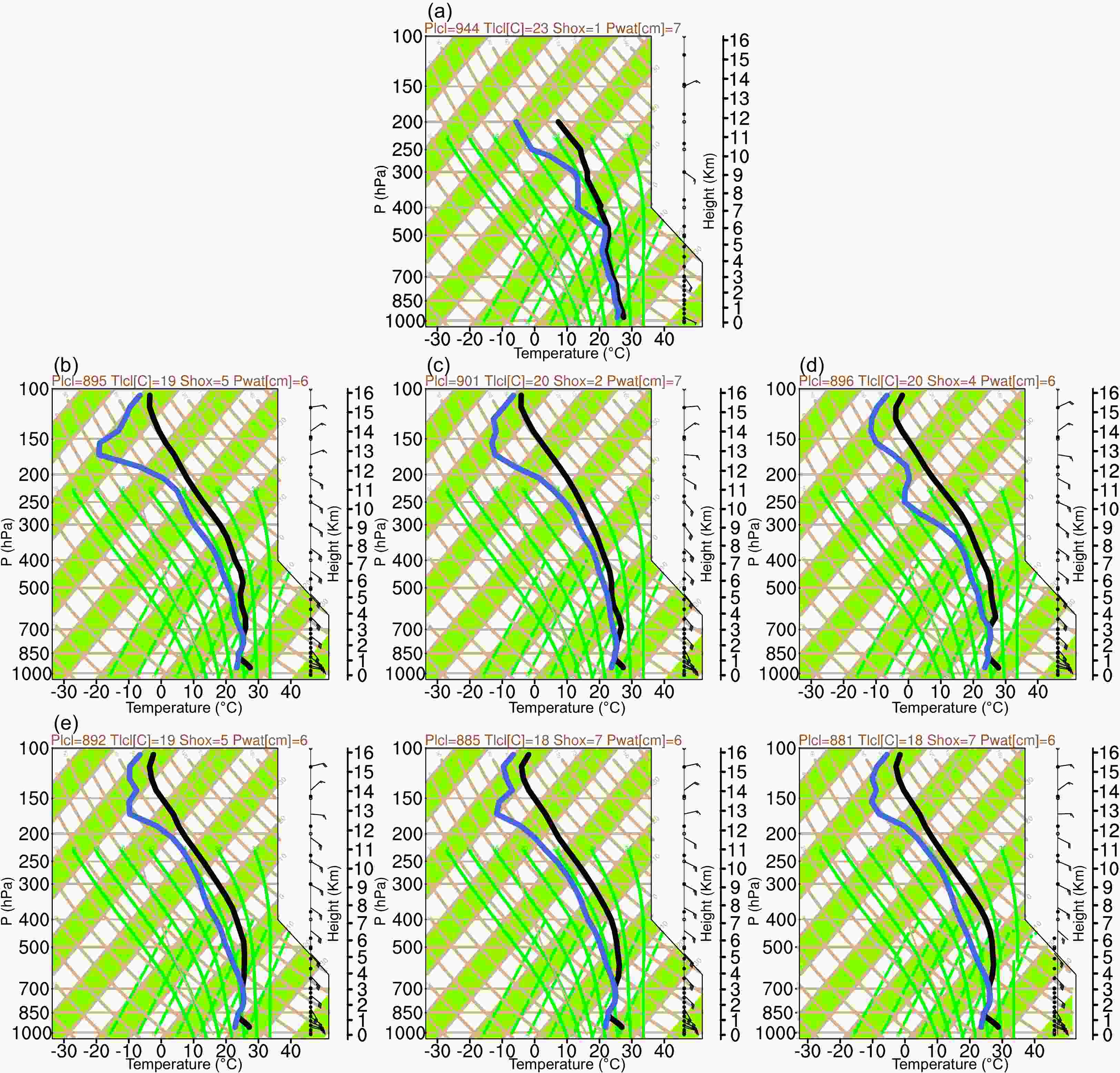
Figure 15. Skew-T plots of the (a) observation and (b) CNTL, (c) PF, (d) MMR, (e) CLM0, (f) CLM01, and (g) CLM012 experiments in Shaowu (27.33°N, 117.47°E) at 1200 UTC 11 July 2018. Plcl: pressure of the lifting condensation level; Tlcl: temperature at the lifting condensation level; Shox: Showalter Index for stability; Pwat: precipitable water.
-
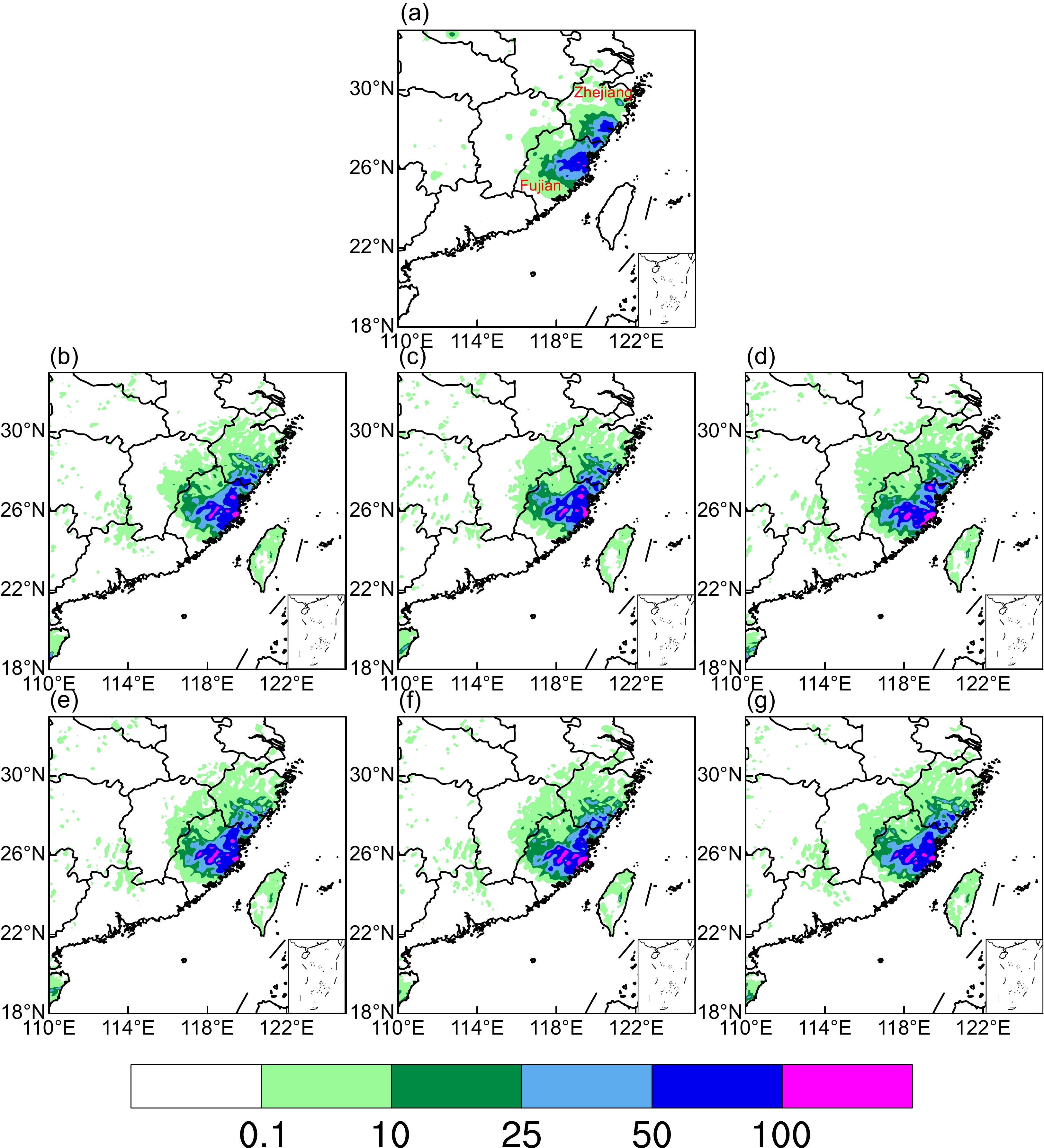
Figure 16 shows the 6-h accumulated precipitation from 0000 UTC to 0600 UTC on 11 July 2018 after the typhoon made landfall. The precipitation observation is from the CLDAS (CMA Land Data Assimilation System) V2.0, which is a grid fusion analysis product evaluated by more than 2400 in-situ national automatic stations of the CMA with a resolution of 0.0625° × 0.0625° (Sun et al., 2020). The observation shows some rainfall centers with values greater than 50 mm along the coast of Zhejiang Province and Fujian Province. In particular, the rainfall center located in Fujian Province has the largest coverage. For all the experiments, the predicted rainfall distributions with values below 50 mm are rather consistent with the observation, while for the rainfall exceeding 50 mm, the rainfall center in the north of Zhejiang Province is largely underestimated. Moreover, the precipitation centers over 50 mm in Fujian Province are situated further north in the CNTL, PF, and CLM012 experiments than in the other three experiments. That is, the MMR, CLM0, and CLM01 experiments mislocated the maximum in Fujian Province. Generally, precipitation exceeding 100 mm is slightly overestimated in all experiments.

Figure 16. The 6-h accumulated precipitation (units: mm) of the (a) observation and (b) CNTL, (c) PF, (d) MMR, (e) CLM0, (f) CLM01, and (g) CLM012 experiments from 0000 UTC to 0600 UTC on 11 July 2018.
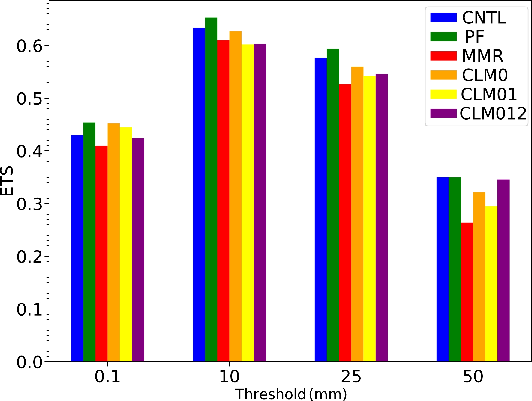
To obtain quantitative verifications of the precipitation forecast, the equitable threat score (ETS) is calculated for comparison. The value of ETS ranges from −1/3 to 1. The higher the score, the better the simulation. Specifically, a score equal to 1 indicates that the simulation totally matches the observation, while a score less than or equal to 0 indicates no forecasting skill (Mesinger and Black, 1992). The ETSs of rainfall forecasts with different thresholds are presented in Fig. 17. The scores for the thresholds of 10 mm and 25 mm are higher than for the other thresholds. Generally, the PF experiment yields the highest ETSs for most of the thresholds (0.1 mm, 10 mm, and 25 mm). For the threshold of 50 mm, the advantage of the PF experiment is negligible since the scores from PF, CNTL, and CL012 are basically comparable.

Figure 17. ETSs of all experiments at different thresholds.
-
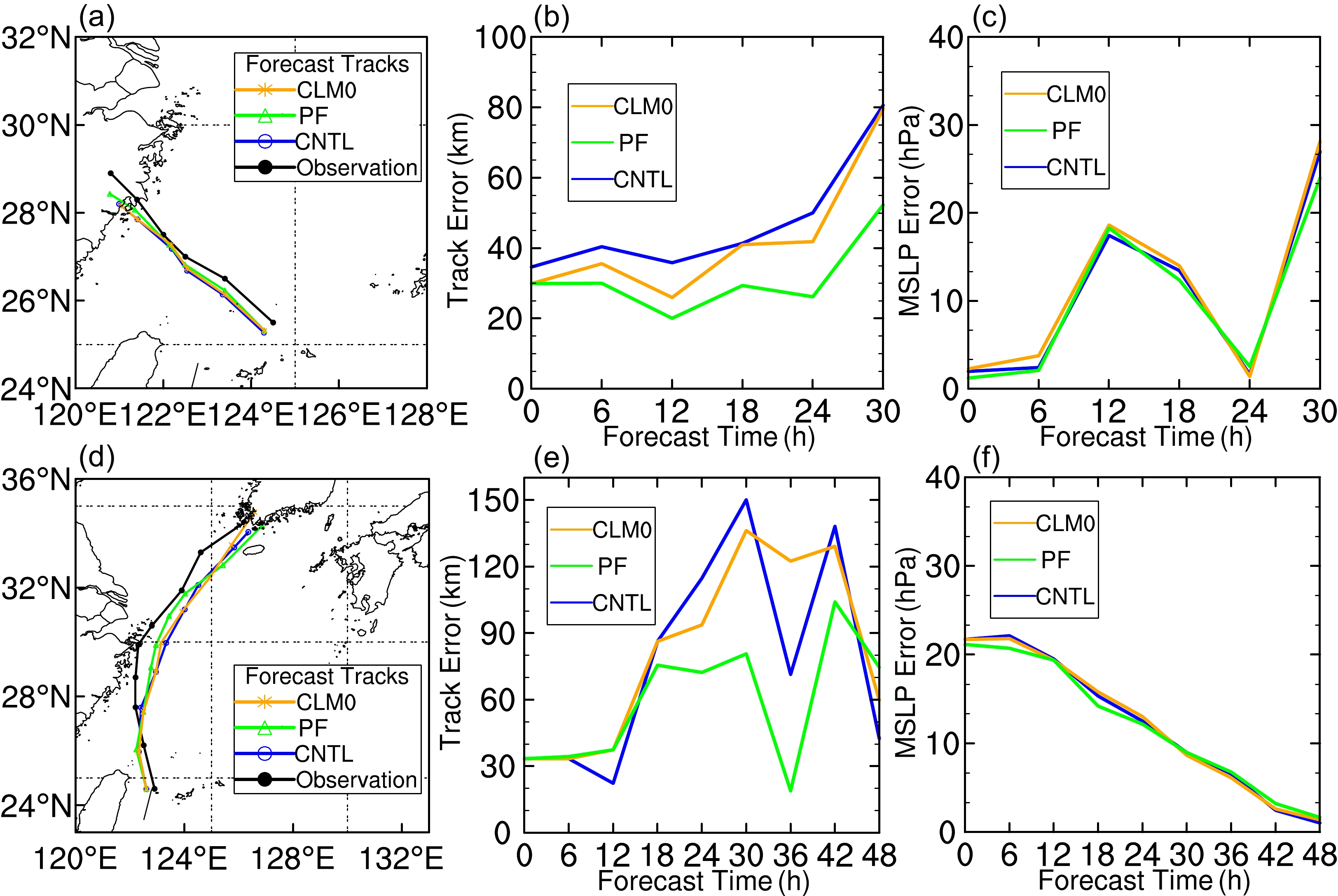
Figure 18 shows the overall verification results for the track forecasts of other cases. For Typhoon Lekima (2019) (Fig. 18a), the tracks of the three experiments are similar when the typhoon is over the ocean. However, due to friction near to where it made landfall, the moving speed of the typhoon in the model decelerates. The PF experiment has a faster vortex moving speed than the other experiments and produces the smallest track error after landfall. Consistently, the track error growth of the PF experiment is slowest, as shown in Fig. 18b. Originally, the gap between the PF and other experiments is 5 km, while the final gap increases to more than 25 km. For Typhoon Mitag (2019) (Fig. 18d), all experiments can simulate the twists in the track of the typhoon. In comparison, the track of the PF experiment matches best with the best track for most of the time. Rapid increases in error can be witnessed in the other experiments (Fig. 18e) after 18 h of model integration, whereas the error of the PF experiment remains almost stable, which results in the maximum error of the PF experiment being obviously smaller than in the other experiments. It should be mentioned that the improvement is rather slight in terms of the intensity forecasts for both Lekima (2019) (Fig. 18c) and Mitag (2019) (Fig. 18f) from the PF experiment. From the temperature, moisture, and dynamical conditions in the analyses and forecasts for Typhoon Lekima (2019) and Mitag (2019) (not shown), it is found that the large improvement in track forecasts can be attributed to the improvement in its surrounding geopotential height environment. It is also noticed that the improvement in the typhoon intensity forecasts is relatively slight when the change in the internal structure of the typhoon in terms of the moisture, temperature, and dynamical condition is limited.
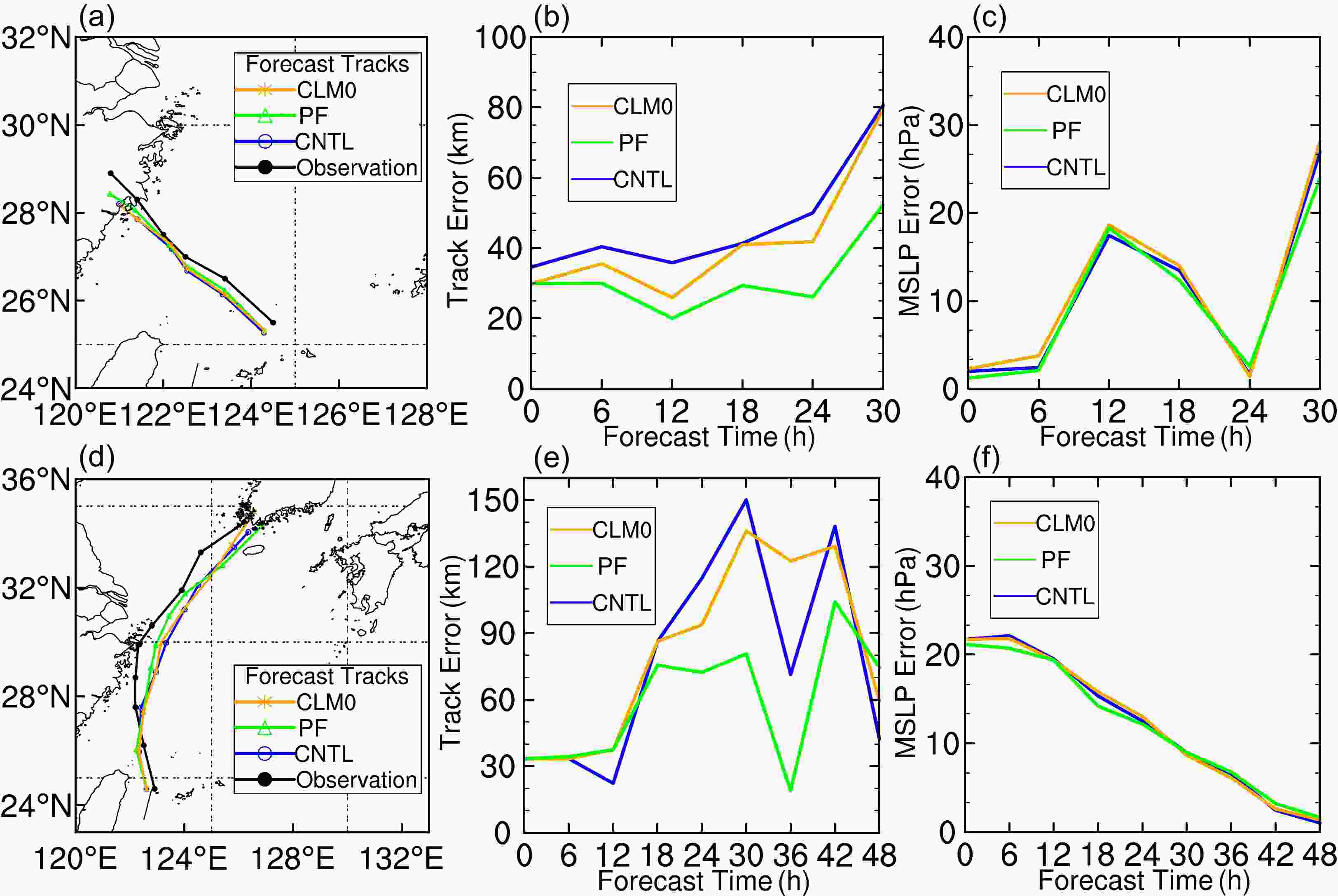
Figure 18. The (a, d) track forecast, (b, e) track error (units: km), and (c, f) MSLP error (units: hPa) for (a–c) Typhoon Lekima (2019) and (d–f) Typhoon Mitag (2019).
-
In this study, the interface for assimilating the new FY-4A AGRI radiance data is completed, and multiple typhoon cases [Maria (2018), Lekima (2019), and Mitag (2019)] are chosen to assess the impact of assimilating the clear-sky FY-4A AGRI vapor channels’ radiances on the analysis and forecast of the three typhoons with the 3DVar method. The benefit of using the PF-based cloud detection approach is examined against the MMR cloud detection scheme, as well as another traditional scheme that directly applies a cloud mask product. Both cloud detection methods identify the cloud signature from the differences between observations and the model benchmark by modeling the cloud in a simple way for each pixel. It is found that more pixels are determined as clear with the PF scheme than with the MMR scheme (2350 versus 1353 for channel 9 and 2155 versus 1239 for channel 10). This indicates that the retrieved cloud height from MMR is generally higher than that from PF, which was also found in Xu et al. (2016). As expected, there is a slightly larger number (about an additional 10%) of pixels for channel 9 than for channel 10 when using the channel-sensitive cloud detection schemes. Besides, the bias correction and quality control of the FY-4A AGRI radiance data are proven to be effective through OMA statistics such as the mean, standard deviation, and root-mean-square converging more to zero.
In general, the assimilation of AGRI radiance has positive effects (compared to the CNTL experiment) for the typhoon and the environment in the Maria (2018) case. The analysis and forecast of those assimilation experiments based on AGRI cloud mask products are comparable with each other and the experiment with the PF cloud detection scheme performs the best. In detail, the analysis from the PF experiment is favorable for the intensification and maintenance of the typhoon, which is demonstrated in terms of the temperature increment, the moisture, and the dynamical conditions for the typhoon with respect to the water vapor increment, sea level field, and vertical cross section. Regarding the forecast, quantitative verifications indicated that forecast skills are improved for the track in the PF experiment, especially after 18 h, which could be explained by better simulating the upper trough. Besides, on average, the overall biases and RMSEs of the PF experiment are closer to zero in all experiments with the assimilation of AGRI radiance, representing fewer forecast errors. On the other hand, the impact of assimilating AGRI radiance data on the typhoon intensity is small. In addition, improved rainfall forecasts from AGRI DA experiments are found, corresponding to the reduced errors of both the thermodynamic and moisture fields, and the improvements at the 25-mm threshold are the most evident. The added value of the AGRI data is further validated with statistical results based on two additional typhoon cases.
Despite encouraging typhoon forecast results having been achieved by assimilating FY-4A AGRI radiance data with the PF cloud detection scheme, further improvements are still needed in terms of typhoon intensity forecasts. In future work, optimizing initial particles and maximizing the synergistic use of multiple channels on geostationary satellites in the PF-based cloud detection algorithm are important aspects. In this study, only clear-sky radiances are assimilated; all-sky radiance assimilation should be further considered to produce better analyses over cloudy and precipitation areas (Zhang et al., 2016; Geer et al., 2018; Otkin and Potthast, 2019; Li et al., 2022a). In addition, new techniques based upon machine learning (Chen et al., 2018) could be applied in the bias correction and quality control procedures, along with more advanced DA methods (e.g., Schwartz et al., 2013; Liu et al., 2020) that apply flow-dependent background error covariances.
Acknowledgements. This research was primarily supported by the Chinese National Natural Science Foundation of China (Grant No. G42192553), Open Fund of Fujian Key Laboratory of Severe Weather and Key Laboratory of Straits Severe Weather (Grant No. 2023KFKT03), the Open Project Fund of China Meteorological Administration Basin Heavy Rainfall Key Laboratory (Grant No. 2023BHR-Y20), the Open Fund of the State Key Laboratory of Remote Sensing Science (Grant No. OFSLRSS202321), the Program of Shanghai Academic/Technology Research Leader (Grant No. 21XD1404500), the Shanghai Typhoon Research Foundation (Grant No. TFJJ202107), the Chinese National Natural Science Foundation of China (Grant No. G41805016), and the National Meteorological Center Foundation (Grant No. FY-APP-2021.0207). We acknowledge the High Performance Computing Center of Nanjing University of Information Science & Technology for their support of this work.
| Typhoon | Model center | Horizontal grid (spacing) (lat×lon) | Vertical levels (pressure top) |
| Maria (2018) | (25°N, 123°E) | 501×401 (9 km) | 57 (10 hPa) |
| Lekima (2019) | (30°N, 123°E) | 381×311 (9 km) | 57 (10 hPa) |
| Mitag (2019) | (30°N, 123°E) | 559×469 (9 km) | 57 (10 hPa) |


 AAS Website
 AAS WeChat