


 DownLoad:


-
Tropical cyclones (TCs) occurring over vast ocean areas often produce heavy rain and can cause severe flooding and losses of life and property when they make landfall. TC precipitation is often a product of the interaction between atmospheric macrodynamic processes and cloud microphysical processes. As the final output of cloud microphysical processes, the horizontal distribution and intensity variations of precipitation are closely related to the phase evolution and structural development of hydrometeors that occur within the weather system. Black and Hallett (1986, 1999) collected aircraft observation data from 230 TCs and proposed a conceptual model of cloud in the eyewall area. It was mentioned that the supercooled water should be located on the inner side of the eyewall area, while the outer side was mostly a mixed phase containing small ice crystal polymers. Due to riming (accretion of liquid water) growth of ice crystals, a large number of columnar cloud ice particles can appear in the mixed layer (0°C–5°C) and be carried out of the eyewall with some snowflakes. During the falling process, they consume a large amount of supercooled water (Wallace and Hobbs, 2006). Hu et al. (2007) using CALIPSO’s lidar depolarization ratio, together with the effective radius, estimated the liquid water content and effective droplet number concentration. Pasqualucci (1984) used ground-based 35-GHz radar and aircraft detection data to obtain the relationship between liquid water content, particle effective radius, and reflectivity in clouds. Frisch (1998, 2002) used radar to detect stratiform clouds over the Atlantic Islands and retrieved the liquid water content in the clouds over the ocean. Sekelsky and McIntosh (1996) explored the effective radius of particles in clouds and the content of ice in clouds using the “dual wavelength ratio” method by channels of 2.8, 33.12, and 94.92 GHz. Shupe et al. (2004) determined the Doppler spectra of supercooled water and ice crystals by searching for spectral peaks in the Doppler velocity spectrum of cloud radar, and inferred the microphysical parameters of stratiform clouds using the reflectivity factor and mean Doppler velocity based on the assumed particle spectrum distribution.
The passive microwave instruments onboard satellites have also become an effective means of detecting precipitation. Wilheit et al. (1977) established the theoretical basis for retrieving precipitation rates from microwave instruments through a relationship between the brightness temperature and precipitation rate. Spencer (1986) noted that the measurements at 37 GHz also carry more information on rain rate and derived a rain rate equation from ground-based radar data over different areas of the world. With the high frequency at 85 GHz, Polarization Corrected Temperature (PCT) has been found to be able to eliminate the contrast between land and ocean, and land precipitation can be obtained from PCT depression (Spencer et al., 1989). Grody (1991) derived a scattering index (SI) based on the 19, 22, and 85 GHz channels of SSM/I to predict the 85 GHz brightness temperatures under clear conditions. This scattering algorithm is still used today in many applications. Kummerow and Giglio (1994) purposed the Goddard Profiling Algorithm (GPROF) to retrieve rainfall and vertical structure from satellite passive microwave sensors. GPROF creates a new hydrometeor profile by obtaining the weighted sum of structures from an a priori database that are consistent with the observed results in radiation measurements. Also, GPROF has been applied to all passive microwave sensors in the GPM constellation.
Since the hydrometeor profiles and precipitation rates retrieved by passive microwave sensors have relatively large errors, space-borne radars are also deployed to provide accurate 3D atmospheric cloud structures. The Tropical Rainfall Measuring Mission (TRMM), launched in November 1997, is equipped with a precipitation measuring radar (PR) in addition to the microwave imager (TMI), which allows for quantification and correction of surface precipitation rates and hydrometeor errors retrieved by TMI. The GPM mission follows the very successful TRMM. In order to increase the capability of measuring frozen and light precipitation that is abundant in higher latitudes, GPM’s dual-frequency precipitation radar (DPR) consists of a 13.6 GHz Ku-band radar similar to TRMM PR and a new 35.5 GHz Ka-band radar. Compared to TMI, GMI has two additional passive microwave bands at frequencies of 165.5 GHz and 183.31 GHz. By combining the observations from the GPM constellation, aided by infrared observations from geostationary satellites, two representative high temporal and spatial resolution mapped precipitation products, the Integrated Multi-satellite Retrievals for GPM (IMERG) and Global Satellite Mapping of Precipitation, from the US and Japan, respectively, are publicly available for various applications (Levizzani et al., 2020).
Although radar can be used to accurately analyze hydrometeors and precipitation under different weather conditions, it is limited by its detection range and cannot perform the retrieval beyond its scan swath. Passive microwave sensors, on the other hand, can observe TC cloud and the distribution of precipitation within a wide scan swath in spite of its lower accuracy. However, there are few algorithms that can simultaneously retrieve precipitation and its hydrometeor profile from passive microwave sensors. This study uses a cloud-dependent 1DVAR algorithm to quantitatively retrieve the TC hydrometeor and precipitation rate. The 1DVAR algorithm uses the Advanced Radiative Transfer Modeling System (ARMS) (Weng et al., 2020) as the observation operator, enabling temperature, water vapor, and clouds to be simultaneously retrieved (Liu and Weng, 2005). It has been shown that the 1DVAR algorithm’s use of cloud-dependent background profiles and error covariance matrices can significantly improve the temperature profiles under TC conditions (Han and Weng, 2018; Hu et al., 2019, 2021). Xu et al. (2023) conducted a further analysis of Typhoon Mekkhala (2020) using cloud-dependent 1DVAR and proposed a cloud scene identification method to describe different weather conditions.
Our previous research mainly focuses on using the 1DVAR algorithm to retrieve temperature and humidity profiles under TC conditions. In this study, we focus on retrieving hydrometeor profiles and precipitation rates using GPM GMI data. The error distribution and possible sources of errors are analyzed. The rest of the paper is organized as follows: Section 2 presents the data sources. Section 3 introduces the 1DVAR retrieval method, including the calculation of precipitation rate, the methods for distinguishing different weather conditions, and the calculation of background error covariance under different weather conditions. Section 4 analyzes the sensitivity of GMI’s different channels to hydrometeors. Section 5 compares the retrieved results for hydrometeors and precipitation rate with DPR, GMI 2A GPROF, and IMERG. Conclusions are given in section 6.
-
The GPM Core Observatory satellite onboard instruments include the DPR and the GMI. The scanning swath width of GMI is 885 km, with 13 channels. The order of the channels from low to high is: 10.65 GHz (V/H), 18.7 GHz (V/H), 23 GHz (V), 37 GHz (V/H), 89.0 GHz (V/H), 166 GHz (V/H), 183.31±3 GHz (V), and 183.31±7 GHz (V). Table 1 shows the instrumental characteristics of GMI. Different frequency bands can effectively detect different types of precipitation, each with specific detection advantages. DPR is the first dual-frequency precipitation radar carried by satellite, which can measure the 3D structure of precipitation, and includes the Ka-band radar (KaPR) and the Ku-band radar (KuPR), with frequencies of 35.5 and 13.6 GHz, and scanning widths of 125 km and 245 km, respectively. The Ku-band radar frequency is similar to that of TRMM PR, but due to technological improvements, KuPR can achieve higher accuracy and sensitivity. The minimum threshold for precipitation detection is 0.5 mm h−1, and when KaPR operates in high sensitivity mode, the minimum threshold for precipitation detection further decreases to 0.2 mm h−1. Besides, the biggest improvement of DPR compared to TRMM PR is its ability to provide quantitative estimates of precipitation particle size distribution for precipitation rates below 15 mm h−1 in the overlapped scanning area of KaPR and KuPR.
GMI channel Central frequency (GHz) Polarization Beamwidth (degree) Footprint (km) 1 10.65 V 1.72 19.4 × 32.1 2 10.65 H 1.72 19.4 × 32.1 3 18.7 V 0.98 10.9 × 18.1 4 18.7 H 0.98 10.9 × 18.1 5 23.8 V 0.85 9.7 × 16.0 6 36.5 V 0.81 9.4 × 15.6 7 36.5 H 0.81 9.4 × 15.6 8 89 V 0.38 4.4 × 7.2 9 89 H 0.38 4.4 × 7.2 10 166.5 V 0.37 4.1 × 6.3 11 166.5 H 0.37 4.1 × 6.3 12 183.31 ± 3 V 0.37 3.8 × 5.8 13 183.31 ± 7 V 0.37 3.8 × 5.8 Table 1. GMI channel characteristics and their specifications of noise.
The IMERG product integrates all passive microwave data from the GPM constellation, with a temporal resolution of 0.5 h and spatial resolution of 0.1° × 0.1°. The GPM-IMERG precipitation product is further divided into three sub-products: “Early Run”, “Late Run”, and “Final Run”. In this study, the Late Run product was chosen as one of the data sources. Furthermore, GPM data could be collected from
https://gpm.nasa.gov/data/directory . -
The cloud-dependent 1DVAR algorithm is based on variational theorem. By inputting satellite observation data, the SI and the cloud liquid water path (CLWP) are calculated to classify weather conditions (section 2.2). Different background profiles (temperature, humidity, cloud liquid water, rain water, graupel) are selected according to weather conditions (convection, stratiform, clear) , and a background error covariance that changes with weather conditions is established (section 2.4). After correcting observation data biases, the algorithm uses incremental calculation and an iterative processes to obtain the atmospheric profile that is closest to the true atmospheric state. Finally, the precipitation rate is calculated based on the iterated hydrometeor profiles (section 2.3).
-
Based on the assumption of a Gaussian distribution and Bayes theorem, the atmospheric variables
$ \mathbf{x} $ can be retrieved by finding the minimum value of J(x), which is the cost function of 1DVAR , and can be written as follows (Hu et al., 2019, 2021):where
$ \mathbf{Y} $ is the observed brightness temperature;$ {\mathbf{x}}_{\rm{b}} $ and$ \mathbf{x} $ represent the background and retrieved variables, respectively; F(x) is the forward operator using$ \mathbf{x} $ as the inputs; O and F represent the error covariances of the instrument and forward operator, respectively; and$ \mathbf{B} $ is the background error covariance matrix. The profile of 1DVAR inversion is the solution that minimizes the cost function mentioned above; that is, taking its derivative and setting it to zero:Then, 1DVAR iteration can be expressed as:
where
$ {\mathbf{x}}_{n} $ denotes the retrieved variables at iteration index n,$ {\mathbf{Y}}^{\mathrm{m}} $ is the observed brightness temperature,$ \mathbf{Y}\left({\mathbf{x}}_{n}\right) $ is the forward operator using$ {\mathbf{x}}_{n} $ as the input;$ {\mathbf{K}}_{n} $ is the Jacobian of$ \mathbf{Y}\left({\mathbf{x}}_{n}\right) $ with respect to$ {\mathbf{x}}_{n} $ under the assumption that$ \mathbf{Y}\left({\mathbf{x}}_{n}\right) $ is locally linear around$ {\mathbf{x}}_{n} $ ,$ \mathbf{E} $ is the error covariance of the forward operator and instrument noise, and$ \Delta {\mathbf{x}}_{n+1} $ and$ \Delta {\mathbf{x}}_{n} $ represent the departure from background vectors at iteration index n+1 and n, respectively. -
In this study, we only focus on cloud detection over oceans in the TC conditions. GMI’s 23.8 and 37 GHz channels are sensitive to the CLWP, which is often used to separate clear sky from cloud scenes (Bormann et al., 2013; Zou et al., 2013; Wu et al., 2019). The CLWP regression coefficients used in this paper are derived from Dou et al. (2020). The SI is based on the brightness temperatures at 23.8 GHz and 85GHz and is also used for cloud classification (Grody, 1991). CLWP and SI are calculated at each field of view (FOV) from observed brightness temperature to categorize weather conditions. The algorithm for estimating the CLWP and SI are expressed as follows:
According to Hu et al. (2019), we classify weather conditions using the following thresholds:
The precipitation rate is calculated as NOAA’s Microwave Integrated Retrieval System (MiRS) from cloud water, rain and graupel by the following formula:
where CLW, RWP and GWP represent the integrated cloud water, rain water and graupel, respectively, and
$ {\mathrm{R}\mathrm{R}}_{\mathrm{C}\mathrm{L}\mathrm{W}} $ is defined as the precipitation rate related to cloud water to improve the retrieval ability of weak rainfall. -
Temperature, humidity and hydrometeors, as well as the surface temperature, are included in background field. For the hydrometeor backgrounds, a climatological background profile is given to the clear, stratiform and convective weather conditions separately, and the background field of temperature and humidity is globally gridded (Hu et al., 2019).
The background error covariance matrix B represents the weight assigned to background field data. The data used to calculate B is the ECMWF short-term forecast atmospheric profile dataset, which contains 25 000 profiles and has 137 pressure levels (Eresmaa and McNally, 2014). We classified different weather conditions using the CLWP and cloud ice water path (CIWP) from the profile set. CLWPs less than or equal to 0.05 kg kg−1 are considered as clear-sky conditions; CLWPs greater than or equal to 1 and CIWPs greater than 0.1 kg kg−1 are treated as convective precipitation; and the remaining FOVs are treated as stratiform precipitation. When creating covariance, we use the cloud ice water content as a substitute since the profile set does not contain the variable graupel. This substitution might represent an uncertainty in the retrieval system. For the atmospheric variables
$ \mathbf{x} $ , the calculation method of$ \mathbf{B} $ is as follows:where
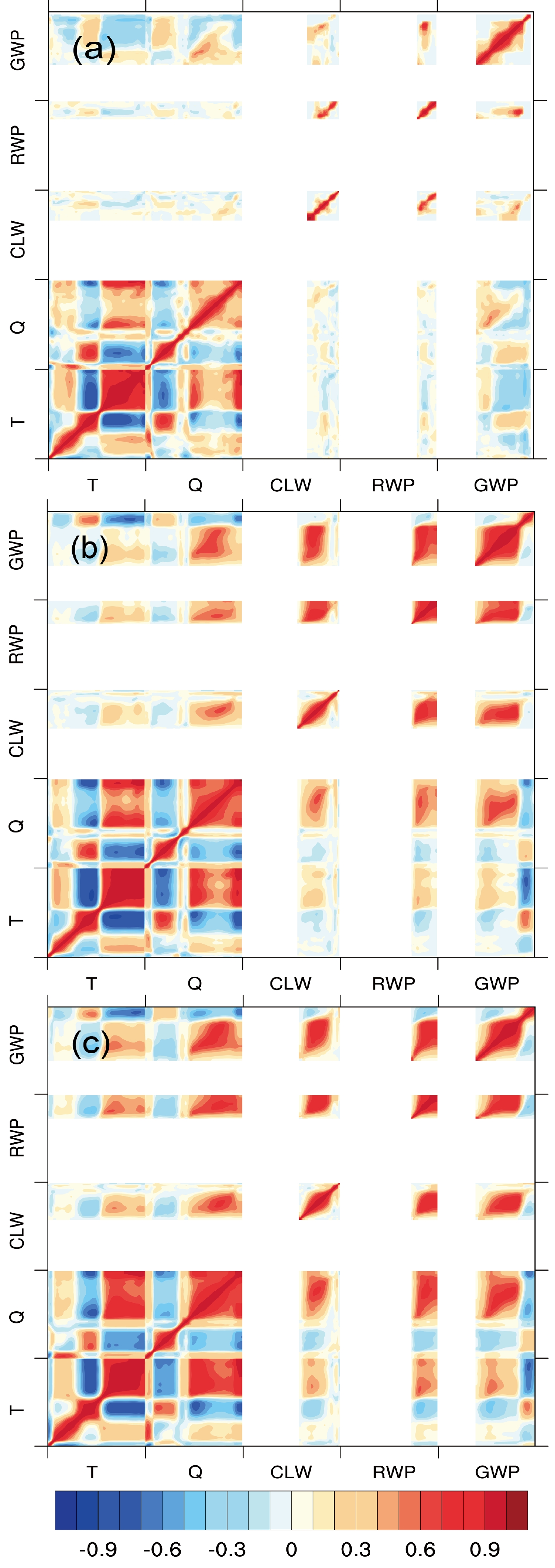
$ {\sigma }_{i,j} $ is the element of row i and column j in$ \mathbf{B} $ ; N represents the number of profiles used to calculate$ \mathbf{B} $ ; and$ {\bar{\mathbf{x}}_{i}} $ and$ {\bar{\mathbf{x}}_{j}} $ represent the average value of x in row i and in column j, respectively. Due to the difference in the magnitude of the different variables, the corresponding correlation coefficients are calculated according to each covariance in the matrix, as shown in Fig. 1, from which we can see that hydrometeors are primarily distributed in the lower troposphere. Under clear-sky conditions, the background error is relatively small. In this case, the algorithm will allocate more weight to the background profile. However, under stratiform or convective conditions, the background error increases, the algorithm assigns less weight to the background profile, and allocates more weight to the observation data accordingly.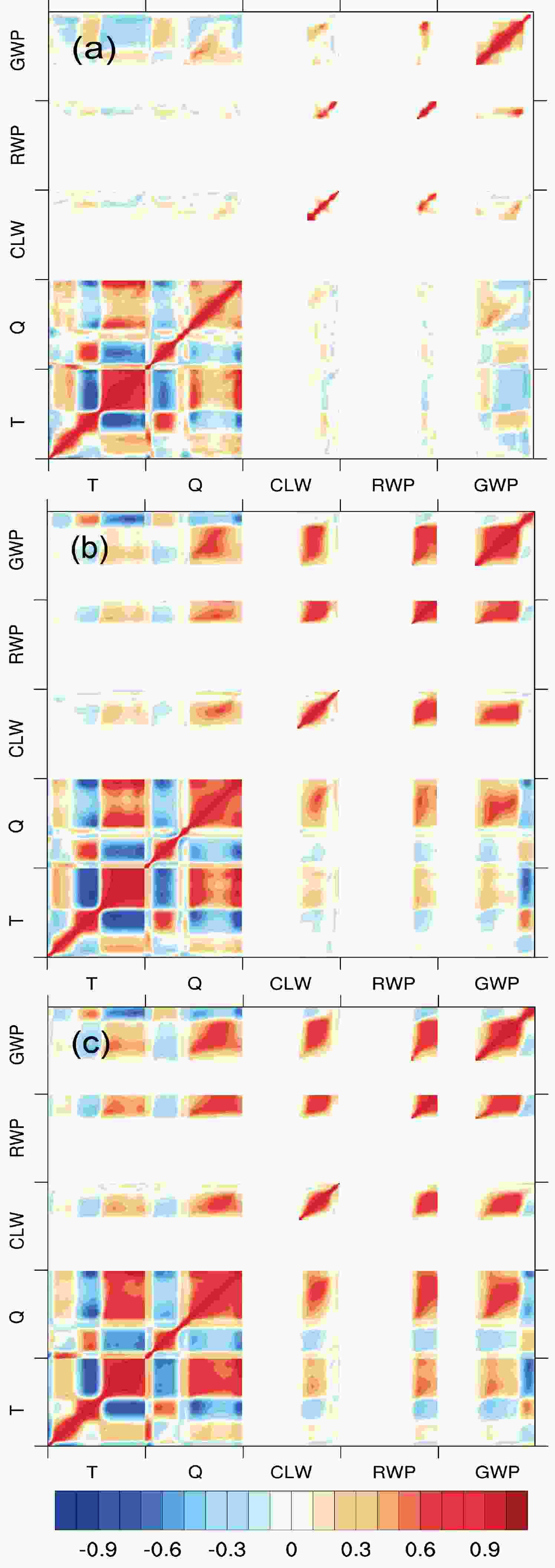
Figure 1. Correlation coefficient under different weather conditions [(a) clear, (b) stratiform, (c) convective] based on background error covariances. The x- and y-axis labels indicate different variables (T, Temperature; Q, Specific humidity; CLW, Cloud liquid water; RWP, Rain water path; GWP, Graupel water path), from 1 hPa to 1000 hPa.
-
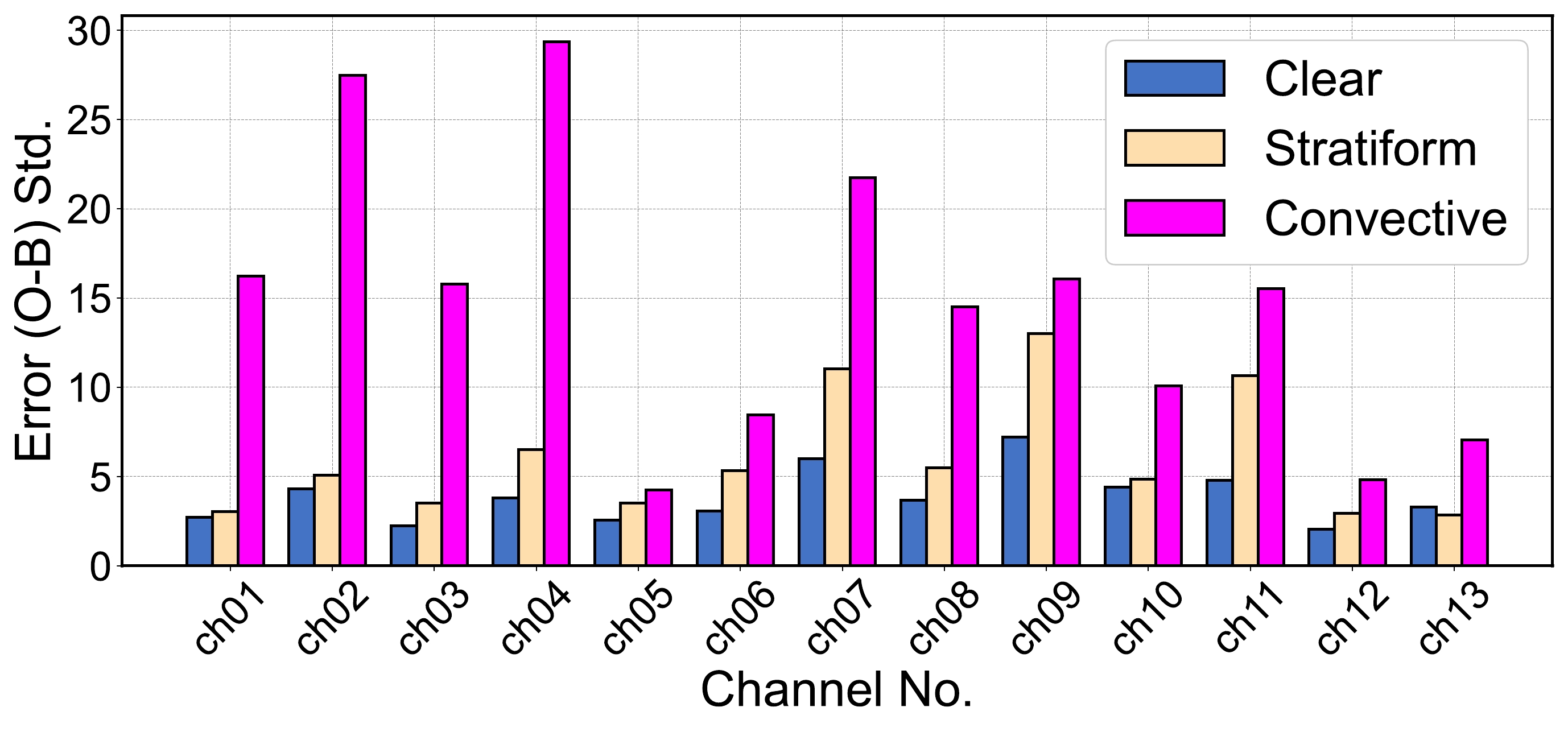
In the 1DVAR algorithm, the value calculated by the observation minus simulation (O-B) and noise equivalent difference temperature (NEDT) for each channel are used as the criteria for determining convergence. Therefore, using ARMS to simulate the brightness temperature of each channel in GMI, the standard deviation of O-B is calculated, and the observation error for each channel is examined for different weather conditions. This study uses the ERA5 dataset with a latitude and longitude range of 50°S to 50°N and 180°W to 180°E to calculate O-B in September 2022. As shown in Fig. 2, it can be seen from the analysis of the O-B deviation under different weather conditions that the scattering effect of hydrometeors in clouds is the dominant effect in the brightness temperature simulation, but the contribution of different types of hydrometeors to the scattering effect needs to be further studied. Moreover, as shown in Fig. 2, the errors of V polarization are smaller than those of H polarization.
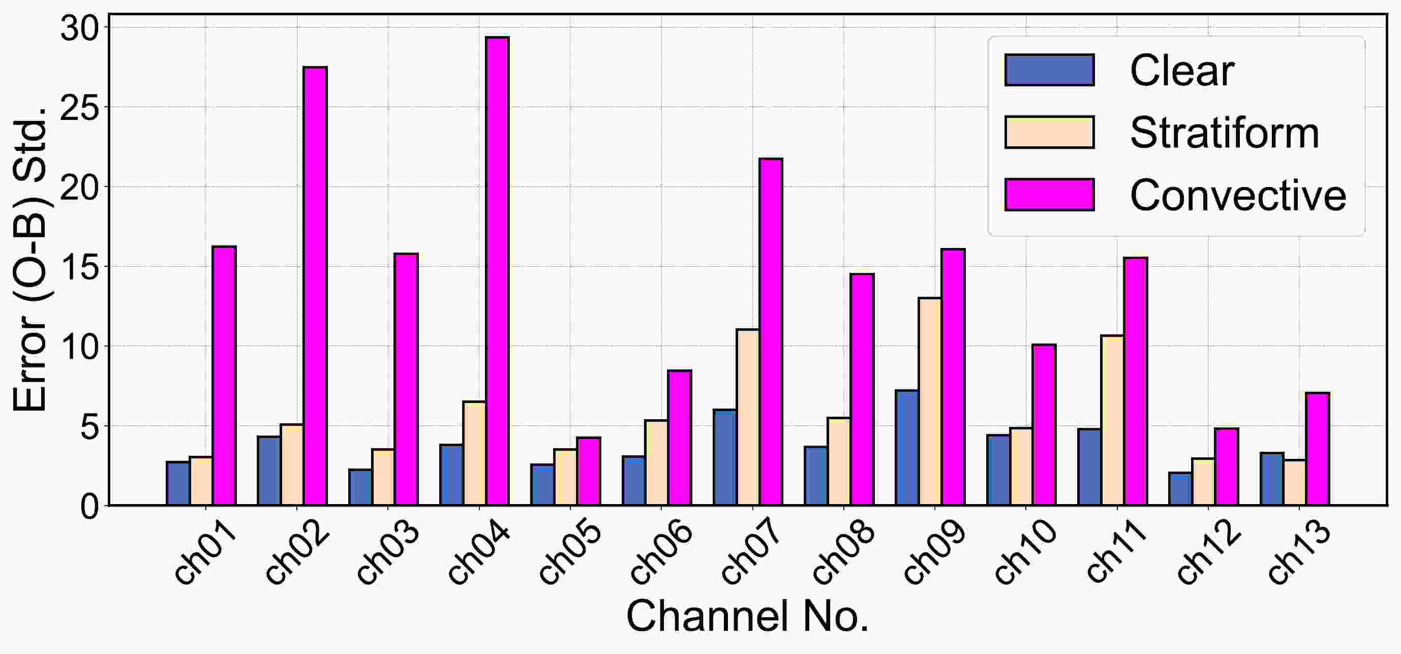
Figure 2. GMI O-B standard deviation under clear (blue bars), stratiform (yellow bars), and convective (pink bars) conditions (units: K).
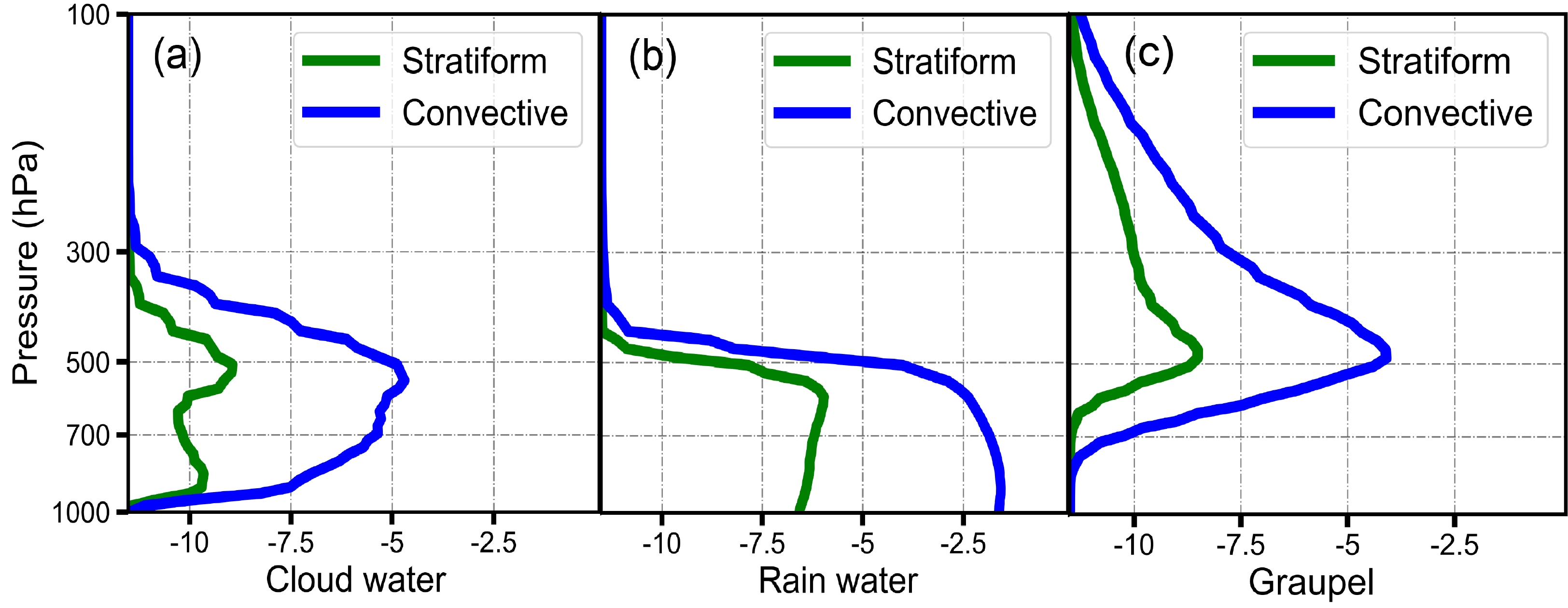
In the 1DVAR algorithm, a climatological background profile is given for each hydrometeor according to scattering conditions. From the background profiles shown in Fig. 3, we can see that cloud water is mainly distributed in the middle and lower troposphere, with a peak height of about 600 hPa; rain water is evenly distributed below 500 hPa; and graupel is slightly higher than the cloud water, peaking at about 400–500 hPa.
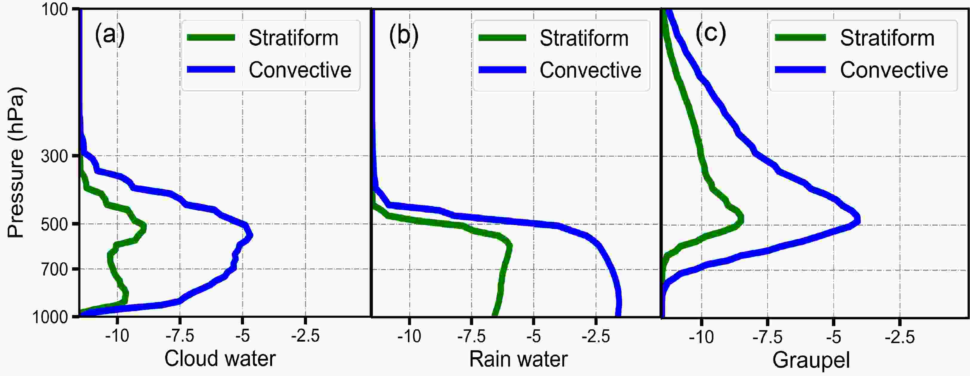
Figure 3. Hydrometeor [(a) cloud water; (b) rain water; (c) graupel] background profiles (green, stratiform; blue, convection). Note that the logarithm is taken for background profiles for better visualization (units: g kg−1).
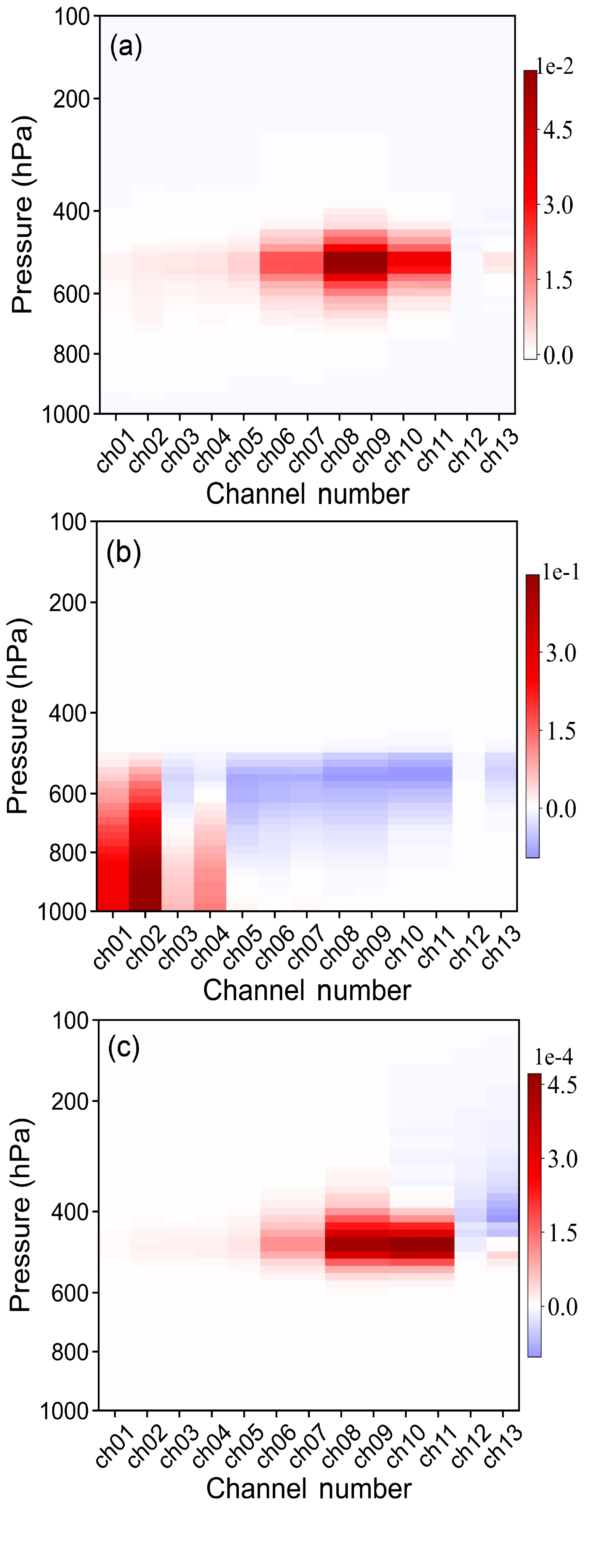
Using the ARMS tangent linear model and hydrometeor background profile, 10% disturbance is given to each hydrometeor layer to analyze the sensitivity of GMI channels to different layers (Fig.4). Channels 5 to 11 of graupel and cloud water produce positive Jacobian, which means the hydrometeor emission exceeding scattering plays a major role. Because the wavelength of channels 1 to 4 are longer, the scattering effect of rain water is smaller, which produce positive Jacobian, while channels 5 to 13 are opposite; the emission of rain water is smaller than the scattering effect. For 183 GHz, graupel exhibits a negative value, indicating that the scattering effect of graupel on 183 GHz is greater than the emission of graupel.
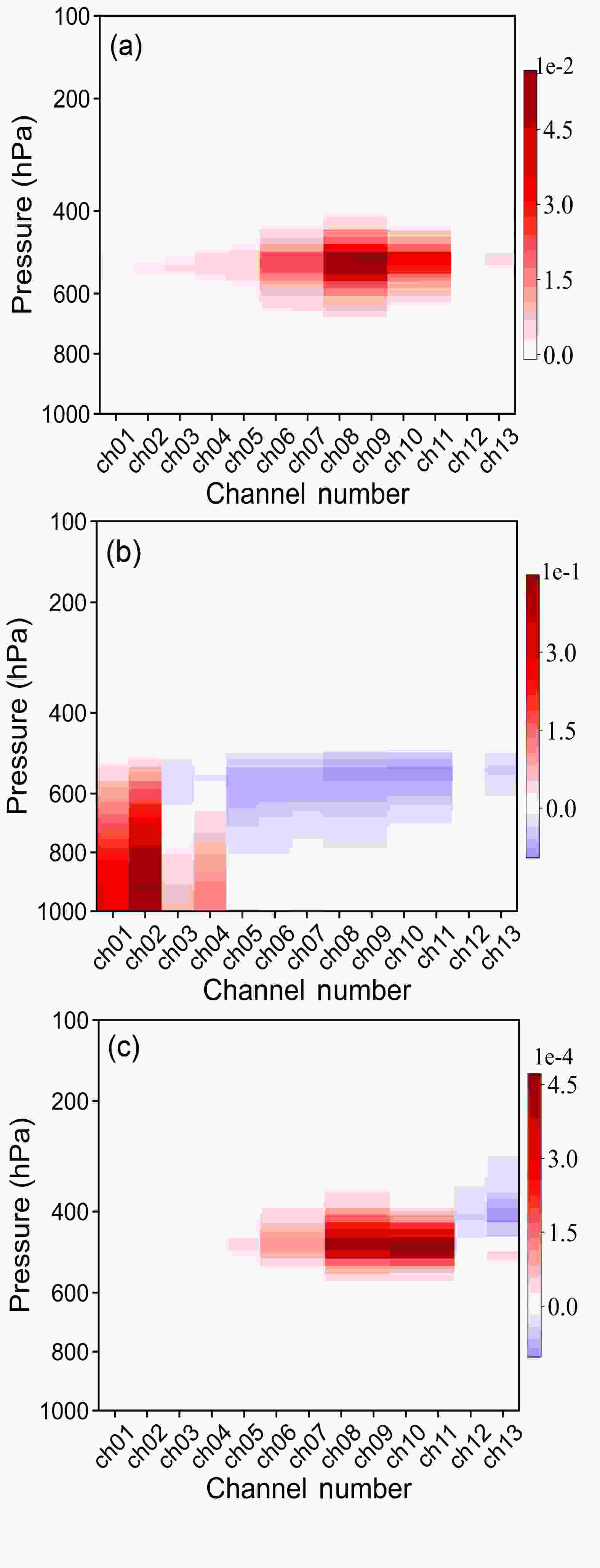
Figure 4. Jacobian calculated by ARMS (units: K): (a) cloud water; (b) rain water; (c) graupel.
Shannon and Weaver (1949) developed information theory by incorporating the entropy of the probability density distribution function, called information entropy. Michele and Bauer (2006) applied information theory to the optimal estimation method and found that entropy can be used to describe the number of independent states in a given state. Therefore, the difference between the entropy of the prior space and the entropy of the optimal estimation space can be equivalent to the new information provided by the observation. The greater the information contributions, the greater the reduction of freedom. Thus, the information content can be obtained by calculating the reduction in degrees of freedom (∆DOF) of the analysis state compared to the prior state. ∆DOF is calculated from:
where I is the identity matrix,
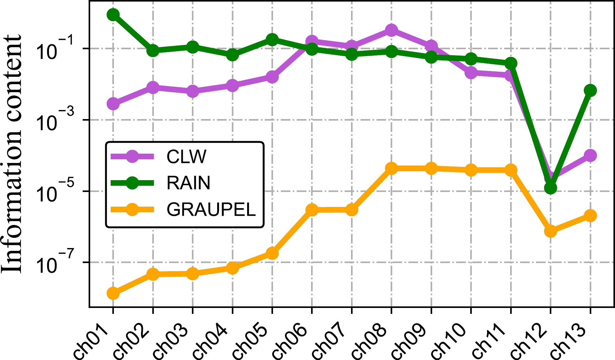
$ {\mathbf{S}}_{\mathrm{r}} $ the analysis error covariance matrix,$ {\mathbf{S}}_{\rm{a}} $ refers to the prior error covariance, and in this study, the background error covariance$ \mathbf{B} $ under the convective conditions mentioned in section 2.3 is used as$ {\mathbf{S}}_{\mathrm{a}} $ , and$ \mathbf{J} $ is the Jacobian matrix of different hydrometeors. Assuming that the observation error is 1K for each channel and there is no correlation between channels,$ {\mathbf{S}}_{\mathrm{y}} $ can be regarded as a diagonal matrix with elements of 1 K2.The sum of ∆DOF for all channels of GMI is 0.79 for cloud water, 1.723 for rain water, and 0.0002 for graupel, which means rain water accounts for the largest amount of information in all GMI channels, while graupel accounts for the least. Figure 5 shows the ∆DOF calculated by all channels of GMI for different hydrometeors. Channels with longer wavelengths contain more information about rain water. Furthermore, channels 6–11 contain more information about cloud water and graupel. Figure 5 suggests that all three hydrometeors have less information in 183 GHz (channel 12, channel 13). Therefore, in this study, only GMI channels 1–11 are used to retrieve the cloud water and precipitation rate.
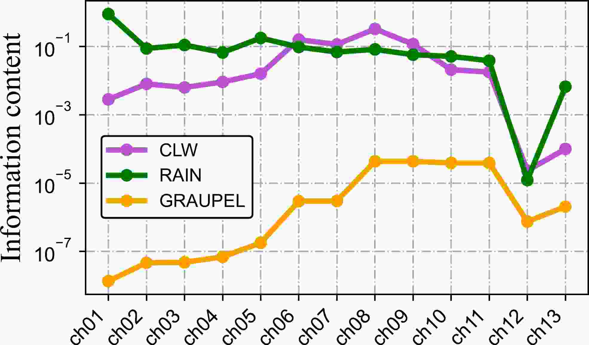
Figure 5. Information content (∆DOF, units: K2) of GMI all channels for three hydrometeors (purple, cloud water; green, rain water; orange, graupel).
-
On 14 September 2022, TC Nanmadol (2022) was generated in the Northwest Pacific Ocean southeast of Kyushu, Japan. On the afternoon of 16 September, TC Nanmadol intensified into a super TC. On 17 September, the TC further strengthened, and Nanmadol reached its peak intensity with 58 m s−1 winds and a minimum pressure of 925 hPa. On 18 September, the TC gradually weakened and made landfall in Japan with a wind speed of 45 m s−1 and a central pressure of 930 hPa. On 20 September, TC Nanmadol merged with a cold front and dissipated. This section uses the GMI observation at 0730 UTC 16 September 2022 to retrieve the TC hydrometeor and precipitation rate. At that time, the central pressure of TC Nanmadol was 955 hPa and the wind speed was 42 m s−1 (Fig. 6).

Figure 6. The track of TC Nanmadol (2022) as reported by the National Hurricane Center. The selected center of TC Nanmadol was located at (23.7°N, 136.0°E), with a central pressure of 955 hPa and minimum pressure of 925 hPa.
-
The TC precipitation rate is estimated from the retrieved cloud water, rain water and graupel. According to the 1DVAR algorithm introduced in section 2, the above three kinds of hydrometeors are retrieved. Due to the high accuracy of DPR products, this section uses DPR products to compare with the retrieved results.
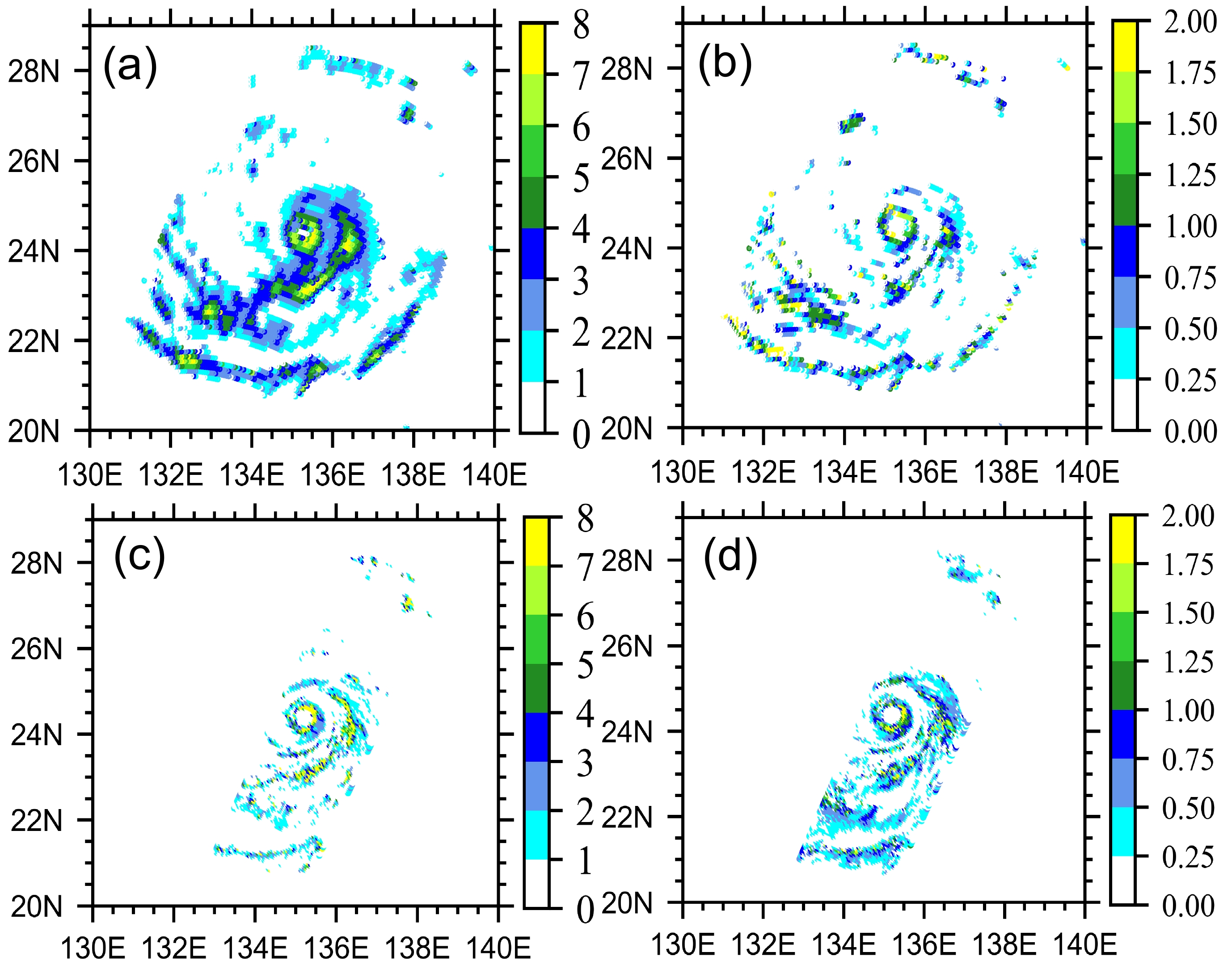
Figures 7a and b show the retrieved vertically integrated spatial distribution of rain and graupel from TC Nanmadol (2022) near 0730 UTC 16 September 2022. The retrieval results show that in the distribution of TC hydrometeors, the rain water content is the highest, followed by graupel, and then cloud water (figure omitted). The three generally exist in the TC precipitation cloud system.
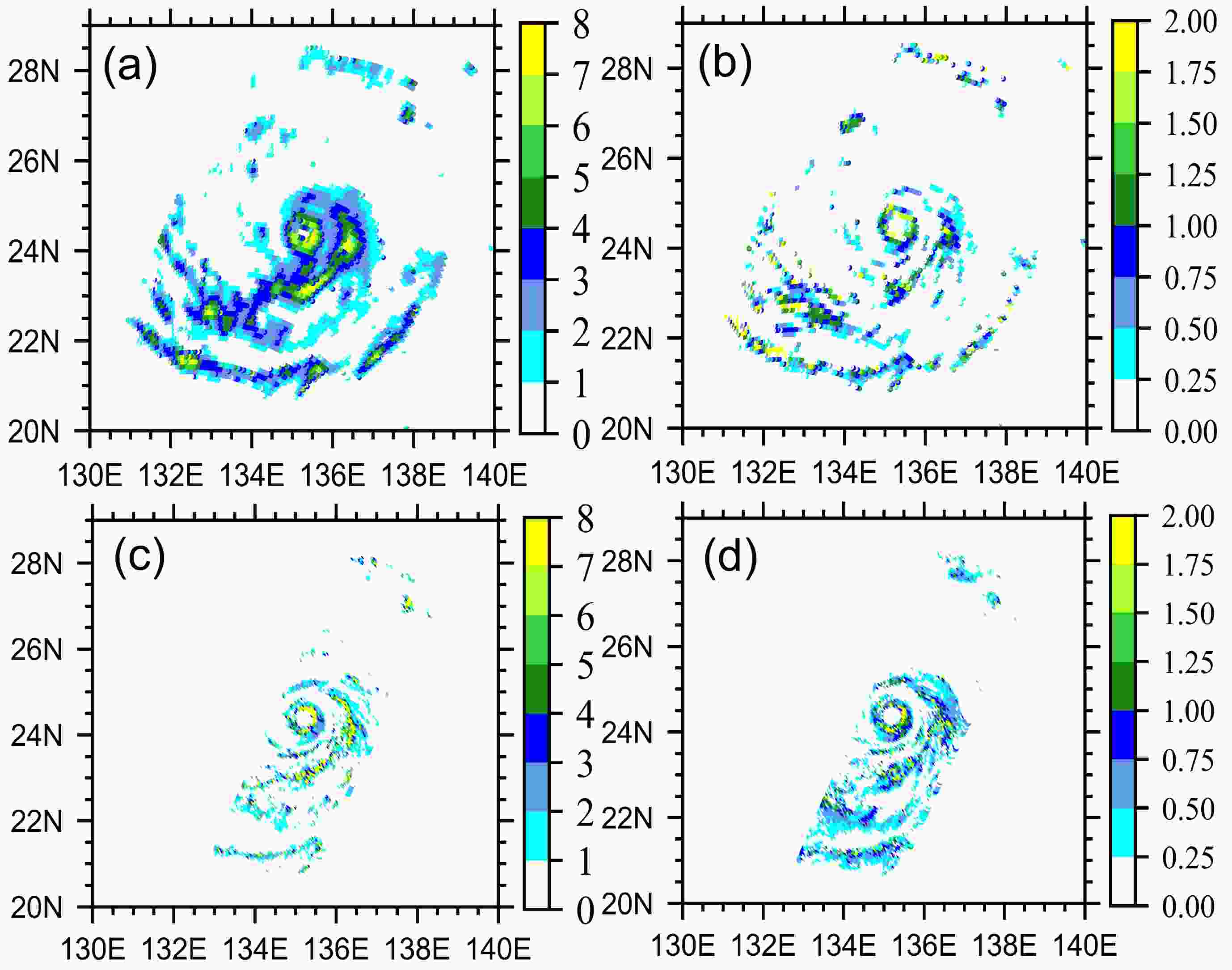
Figure 7. TC Nanmadol (2022) spatial distribution of 1DVAR-retrieved vertically integrated (a) rain water, (b) graupel, (c) DPR liquid precipitation, and (d) DPR non-liquid precipitation at 0730 UTC 16 September 2022 (units: kg m−2).
Compared with the vertical integration of DPR liquid water in Fig. 7c, the rainwater range retrieved by the 1DVAR algorithm is larger but the location and intensity of the 1DVAR-retrieved rain water are relatively consistent with those of the DPR liquid water. Since there is no separate graupel product in the DPR product, the vertical integration of non-liquid water (Fig. 7d) is compared with the 1DVAR-retrieved graupel. It can be seen that the positions of high-value areas of the two are basically the same.
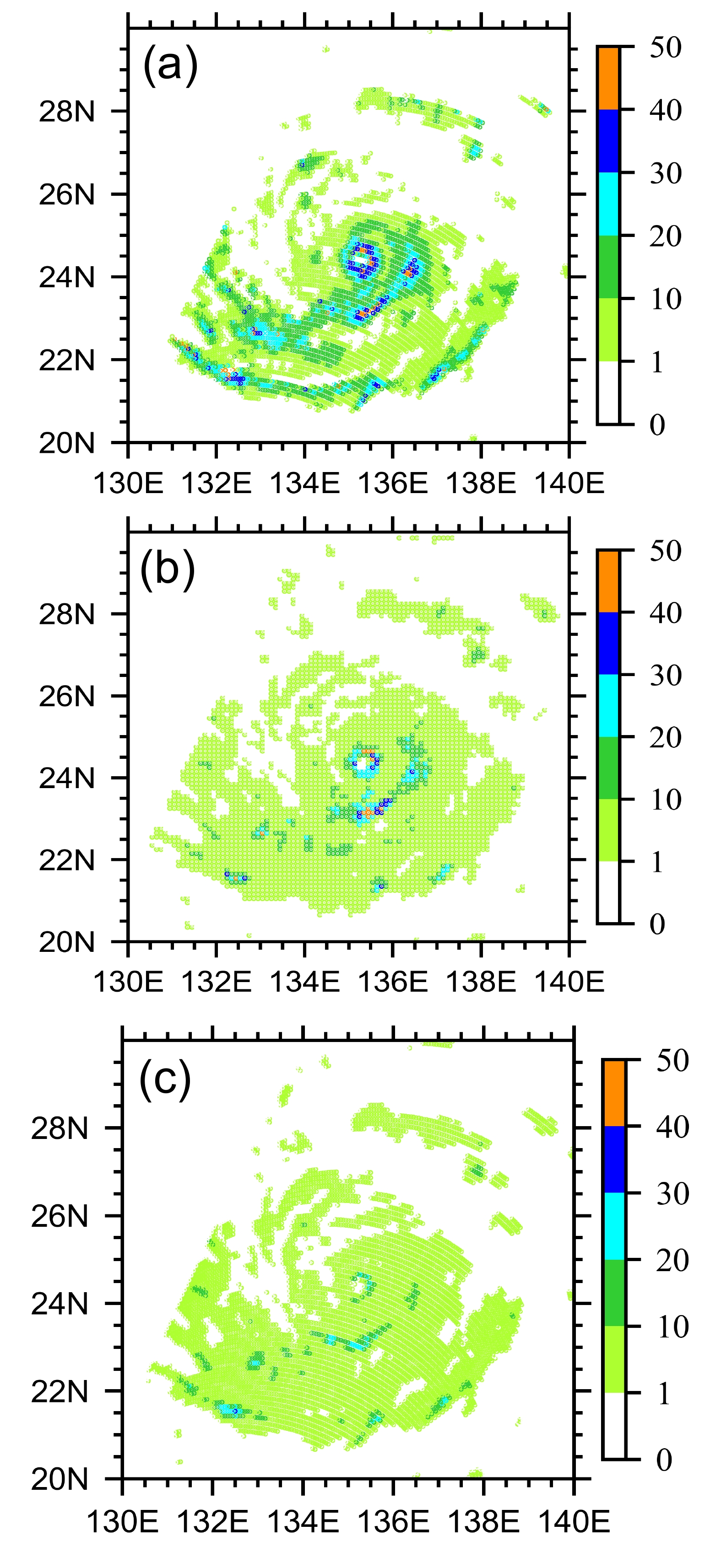
The retrieved result of precipitation rate is shown in Fig. 8a. Compared with the IMERG precipitation rate product (Fig. 8b), the 1DVAR algorithm overestimates the precipitation around the rain band, which is consistent with the retrieved error of rain water, indicating that the retrieved error of rain water is the main reason for the retrieved error of precipitation rate. Also, the GMI 2A product underestimates the precipitation of the rain band compared to the IMERG product. Adhikari (2019) conducted a statistical analysis of GMI 2A GPROF data from April 2014 to March 2018, analyzing the retrieval results of GMI 2A GPROF for weather systems of different scales. It was found that the GMI tends to underestimate the precipitation volume for systems within 200 km2. This is consistent with the comparison results in this paper.
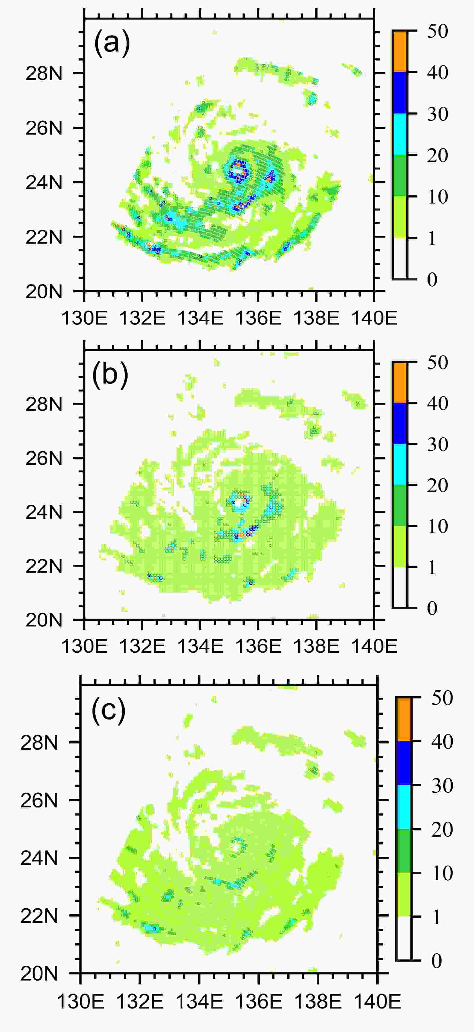
Figure 8. Spatial distribution for TC Nanmadol (2022) of precipitation rates (units: mm h−1) retrieved from (a) the 1DVAR algorithm, (b) IMERG Late Run, and (c) GMI 2A GPROF, at 0730 UTC 16 September 2022.
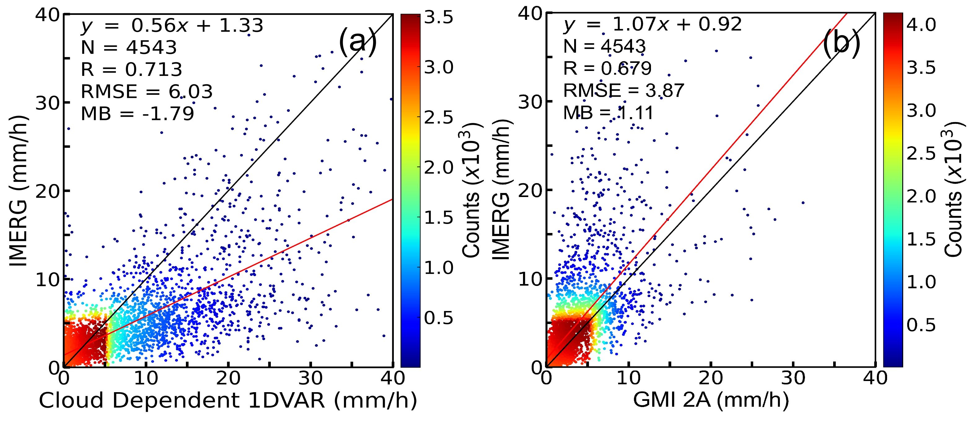
Due to the fact that TC Nanmadol mainly occurred over the ocean from 15–17 September 2022, GMI data from these three days were used for precipitation rate retrieval and statistics, in order to obtain a more accurate analysis of the precipitation rate during the TC process. The precipitation rate obtained from the 1DVAR algorithm and the GMI 2A product were reprojected and matched with the IMERG precipitation product, and 4543 grid points were selected where all three types of data were available. The 1DVAR and GMI 2A product were compared with the IMERG precipitation rate, as shown in Fig. 9. Both the 1DVAR and GMI 2A product have the most precipitation rate data below 5 mm h−1, and the precipitation points become more scattered as the precipitation level increases. The 1DVAR algorithm has a larger systematic bias compared to the GMI 2A product, but the correlation coefficient between the 1DVAR algorithm and IMERG algorithm is higher at 0.71, while that of GMI 2A is 0.68. The variance (RMSE) and mean bias (MB) of the GMI 2A product are both smaller than those of the 1DVAR product, at 3.87 mm and 1.11 mm, respectively, while the 1DVAR algorithm has an RMSE and MB of 6.03 mm and −1.79 mm, respectively.
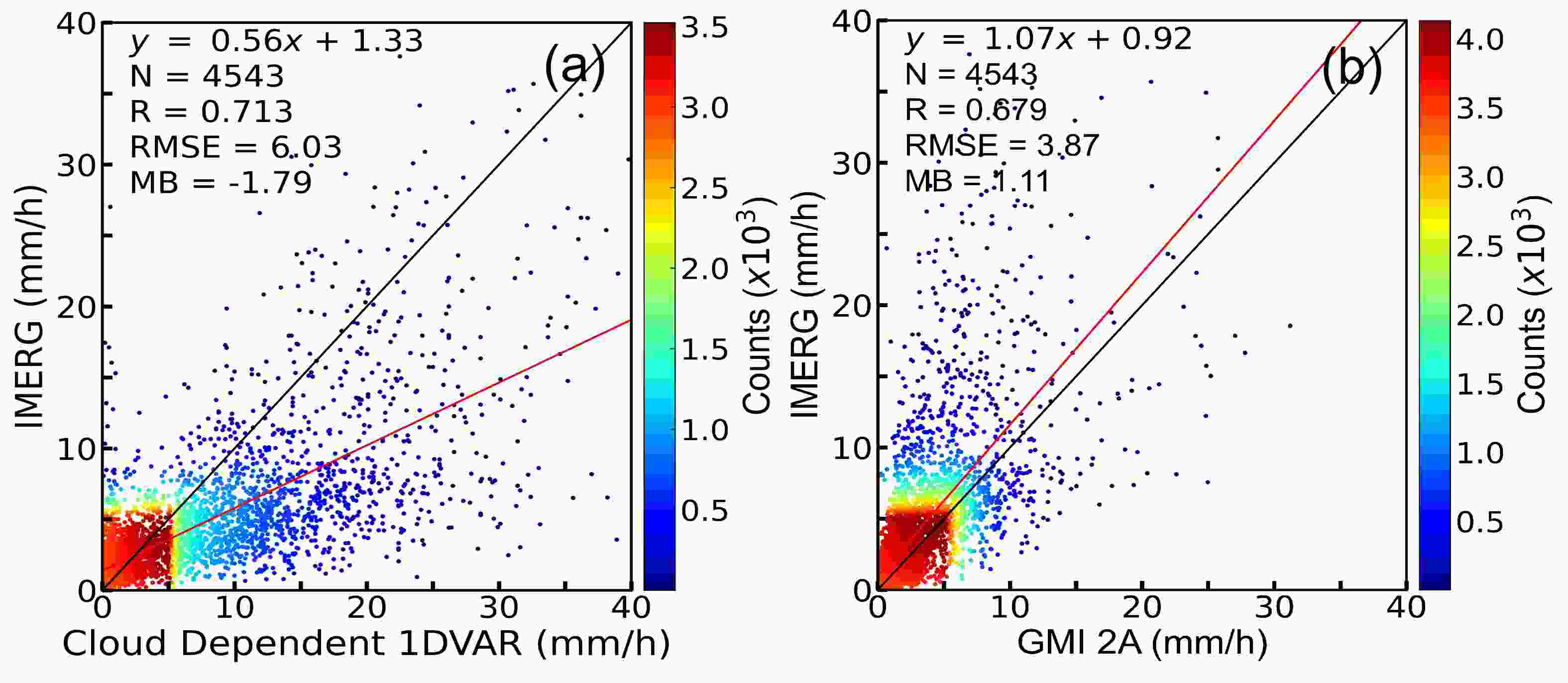
Figure 9. Scatterplots of matched precipitation rates (units: mm h−1) (a) between IMERG and 1DVAR, and (b) between IMERG and GMI 2A, on 15–17 September 2022 (20°–30°N, 130°–145°E).
In conclusion, the rainwater range retrieved by 1DVAR is larger, which causes the retrieved precipitation range to be larger, and to exhibit obvious systematic errors. Compared with the GMI 2A precipitation rate product, the correlation coefficient between the 1DVAR precipitation rate and the IMERG product is higher. In general, the 1DVAR algorithm is accurate in retrieving the location and structure of TC precipitation, but the retrieval of precipitation intensity is not very accurate.
-
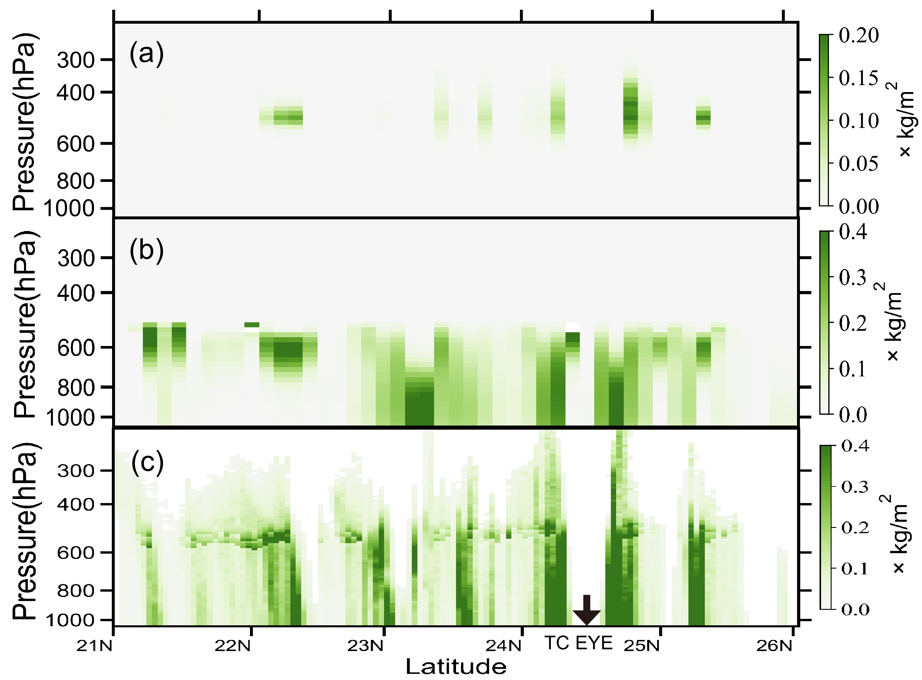
As the precipitation rate is based on the retrieval results of cloud water, rain water and graupel, the vertical distribution of these hydrometeors is further analyzed. Figures 10a–c display the vertical distributions of retrieved graupel, rain water, and the DPR precipitable water product, respectively. They all pass through the typhoon eye wall. The latter includes the content of liquid water and non-liquid water. It can be seen from Fig. 10 that graupel is distributed above the melting layer. Due to its high condensation growth rate, more latent heat is released, which is conducive to the further development of the system. In addition, the rain water can be formed more by the melting of the ice-phase particles above the 0°C layer (Rosenfeld et al., 2007, 2012; Jiang et al., 2016). The retrieved graupel is consistent with the large-value area above the DPR precipitable water product melting layer.
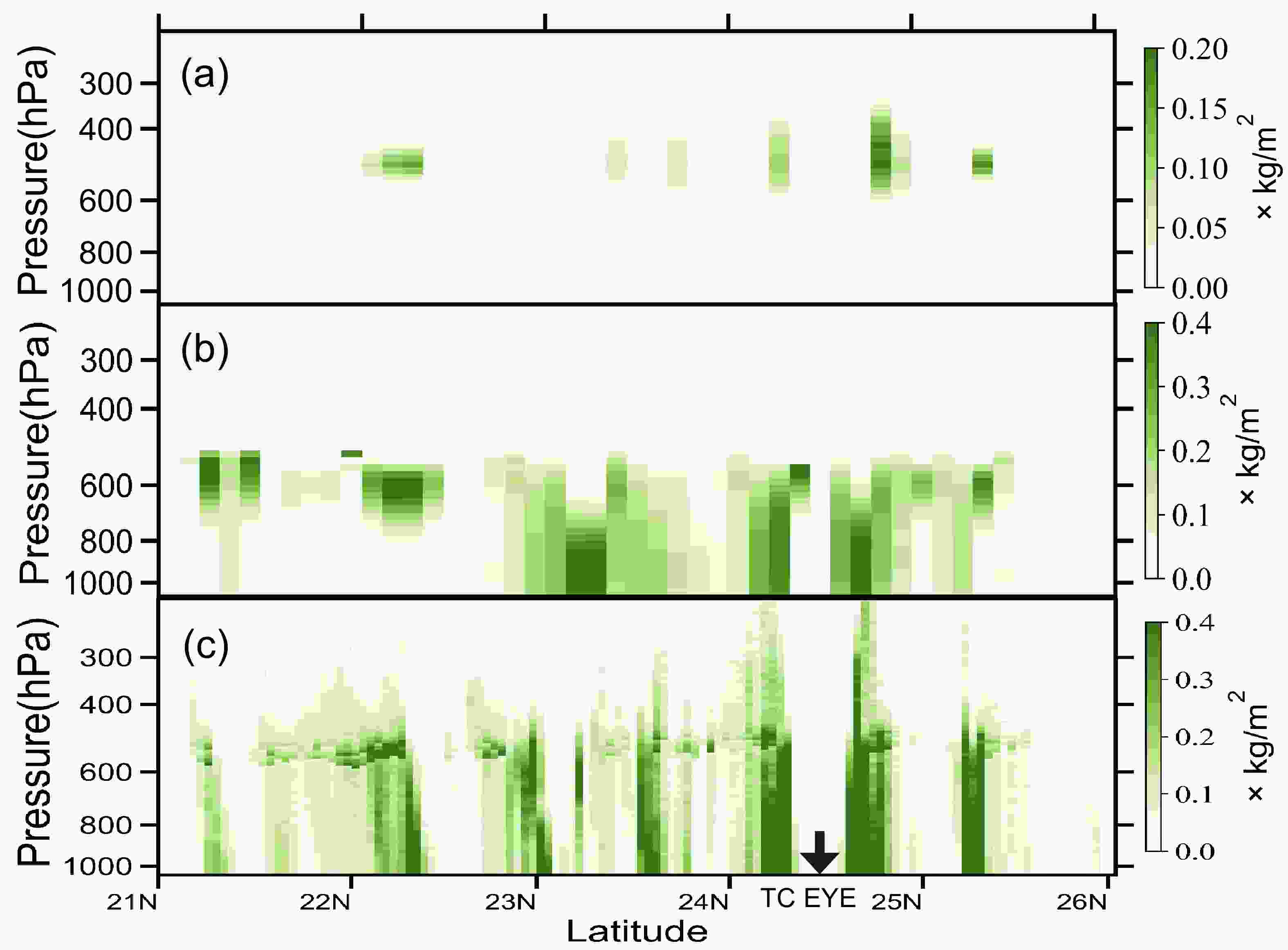
Figure 10. Vertical distribution of (a) 1DVAR-retrieved graupel, (b) 1DVAR-retrieved rain water, and (c) DPR precipitable water product, for TC Nanmadol (2022) at 0730 UTC 16 September 2022 (units: kg m−2).
As shown in Fig. 10c, the rain water is mainly distributed in the TC eyewall and its rainband. The discontinuous points in Fig. 10c indicate the location of the melting layer. Comparing the 1DVAR-retrieved rain water with the DPR precipitable water product, it can be seen that the rain water retrieved by the 1DVAR algorithm under the melting layer at 21°–23°N and 25°–25.5°N is much smaller compared to the DPR product, indicating that the 1DVAR-retrieved rain water (Fig. 10b) under the melting layer in the rain band is not well retrieved.
In the comparison between the 1DVAR-retrieved results and the DPR products, DPR has a good retrieval effect on the rain water under the melting layer and the graupel above it. Therefore, in this section, the DPR Ka and Ku vertical profiles passing through the eye of the TC are further analyzed (as shown in Fig. 11), which is the 11th scanning position of DPR
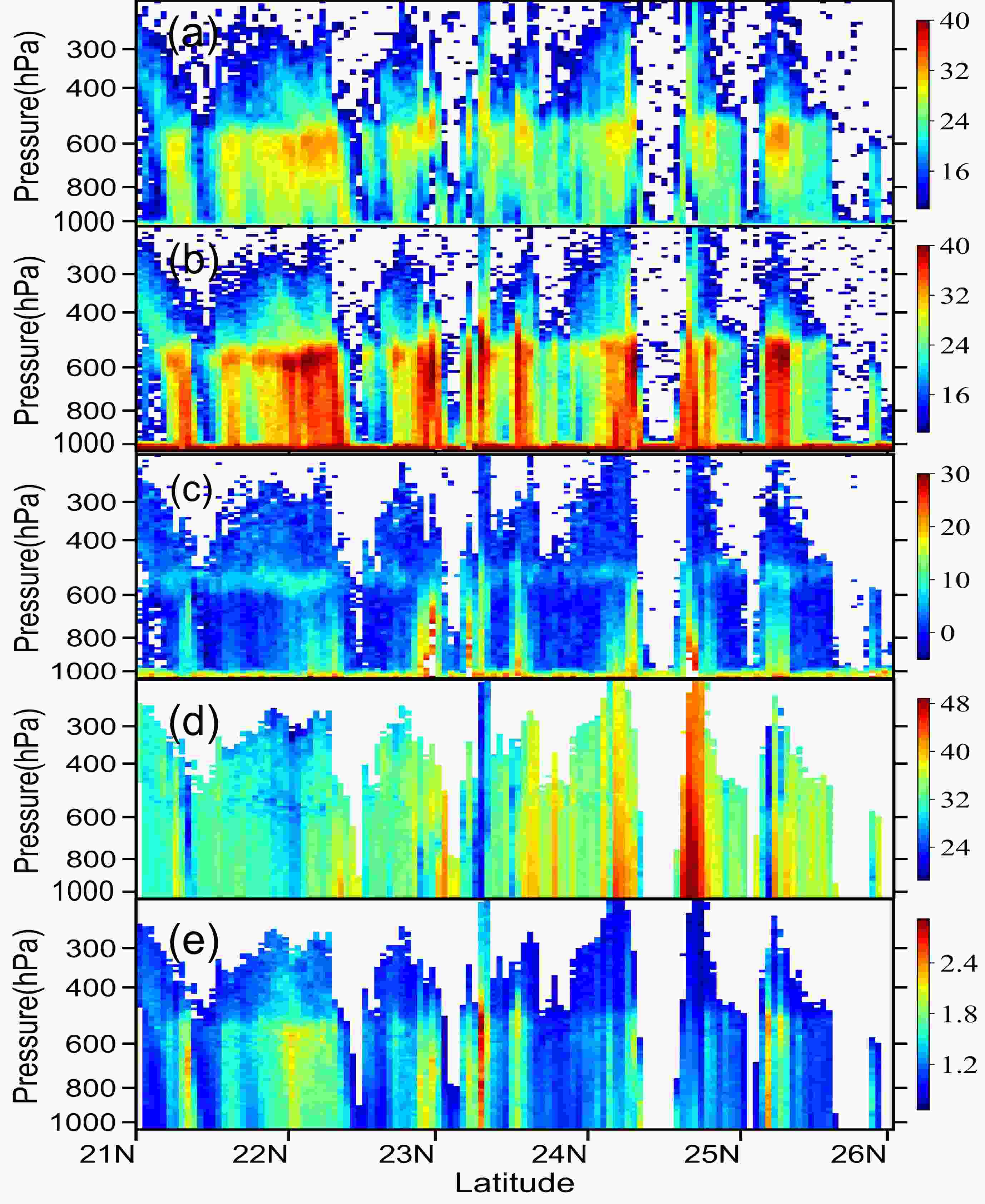
Figure 11. Vertical distribution of the (a) DPR Ka-band (units: dBZ), (b) DPR Ku-band (units: dBZ), (c) dual-frequency difference (Zm,Ku − Zm,Ka) (units: dBZ), (d) 10lgNw (particle concentration, obtained from the DSD), and (e) Dm (particle diameter, obtained from the DSD; units: mm).
As shown in Figs. 11a–e, near the eyewall of the TC, the height of the echo top is the highest, indicating that the convection is developing vigorously at this time. Since the Ka wavelength is shorter than the Ku wavelength, the Ka band attenuates most near the melting layer. As shown in Fig. 11c, The difference between the Ku band measured reflectivity factor and the Ka band measured reflectivity factor (Zm,Ku − Zm,Ka) shows the location of melting layer and the area with the highest rain intensity, and their positions are consistent with the DPR precipitable water product. Comparing Figs. 11e–e, it can be seen that during the TC precipitation process, the particle size is between 1.5 and 2.6 mm. The particle size near the eyewall is smaller than other rain bands in this process, but the particle number concentration (Nw) obtained from the drop size distribution (DSD), is the highest. Meanwhile, the particle diameter (Dm) obtained from the DSD increases significantly below the melting layer of the spiral rain band, which may be one of the main reasons for the much smaller retrieval results of 1DVAR on the rain water below the melting layer. Therefore, the DPR Ku and Ka frequency has the potential to improve the retrieved effect of the rain water below the melting layer.
It can be seen from the above that the 1DVAR algorithm overestimates the rainwater content and underestimates the rain water below the melting layer of the spiral rain belt. These two reasons together lead to a high retrieved precipitation rate. Comparison with DPR DSD products revealed that there was a significant increase in particle size below the melting layer in the spiral rain band, which may be one of the main reasons for the much smaller retrieval results of 1DVAR on the rain water below the melting layer. Therefore, by changing the setting of the particle radius or scattering tables in the 1DVAR retrieval process through DPR, the retrieval effect of precipitation may be improved.
-
In this study, GMI brightness temperature and a cloud-dependent 1DVAR algorithm were used to retrieve the hydrometeors and precipitation rate of TC Nanmadol (2022). Compared with GMI 2A precipitation rate products, the overall volume of the cloud-dependent 1DVAR precipitation rate is higher. However, the cloud-dependent 1DVAR precipitation rate has a higher correlation coefficient with the IMERG product at 0.713, while the GMI 2A correlation coefficient is 0.679. In general, the cloud-dependent 1DVAR algorithm is accurate in retrieving the location of TC precipitation.
In the cloud-dependent 1DVAR algorithm, the precipitation rate is based on the retrieval results of cloud water, rain water, and graupel. Therefore, accurate retrieval of the hydrometeor profile is required. According to the background profile of hydrometeors, rain water is uniformly distributed in the lower part of the troposphere, while graupel is distributed above the cloud water. According to the O-B deviation under different weather conditions, the scattering effect of these hydrometeors in clouds is the main factor affecting the brightness temperature simulation, and accurately simulating the scattering of hydrometeors in the radiative transfer model requires further investigation. Though analyzing the sensitivity of different GMI channels to different hydrometeors, we found that under convective conditions, rain water accounts for the largest volume of information in all GMI channels (∆DOF = 1.72), while graupel accounts for the least (∆DOF = 0.0002), and all three hydrometeors have less information in 183 GHz. According to the Jacobian, under convective conditions, the cloud water emission of all channels of GMI is greater than the scattering. For rain water, channels 1–4 have greater emission than scattering, while channels 5–13 scatter more than they emit. For graupel, channels 12 and 13 scatter more than they emit, while for other channels, emission is greater than scattering.
According to the DPR reflectivity, both the Ku and Ka band have the highest echo top near the eyewall, indicating strong convection. The Ka-band attenuation is severe near the melting layer, as compared with the Ku-band. The double frequency difference reflects the location of the melting layer and the area of strong attenuation. Comparing the retrieved hydrometeors with DPR products, the cloud-dependent 1DVAR algorithm is not effective for retrieval of rain water below the melting layer in a spiral rain band. The DPR DSD product shows that there is a significant increase in particle size below the melting layer in the spiral rain band, indicating particle size may affect the 1DVAR retrieval effect of rain water. Therefore, updating the scattering tables or using more accurate background profiles in the 1DVAR algorithm may improve the retrieval effect.
Acknowledgements. This study was funded by the National Key Research and Development Program of China (Grant No. 2022YFC3004202) and the National Natural Science Foundation of China (Grant Nos. U2142212 and 42105136).
| GMI channel | Central frequency (GHz) | Polarization | Beamwidth (degree) | Footprint (km) |
| 1 | 10.65 | V | 1.72 | 19.4 × 32.1 |
| 2 | 10.65 | H | 1.72 | 19.4 × 32.1 |
| 3 | 18.7 | V | 0.98 | 10.9 × 18.1 |
| 4 | 18.7 | H | 0.98 | 10.9 × 18.1 |
| 5 | 23.8 | V | 0.85 | 9.7 × 16.0 |
| 6 | 36.5 | V | 0.81 | 9.4 × 15.6 |
| 7 | 36.5 | H | 0.81 | 9.4 × 15.6 |
| 8 | 89 | V | 0.38 | 4.4 × 7.2 |
| 9 | 89 | H | 0.38 | 4.4 × 7.2 |
| 10 | 166.5 | V | 0.37 | 4.1 × 6.3 |
| 11 | 166.5 | H | 0.37 | 4.1 × 6.3 |
| 12 | 183.31 ± 3 | V | 0.37 | 3.8 × 5.8 |
| 13 | 183.31 ± 7 | V | 0.37 | 3.8 × 5.8 |


 AAS Website
 AAS WeChat