


 DownLoad:


-
Dynamical downscaling is a crucial approach to generating high-resolution climate information that is consistent with physical principles. This information is essential for climate-related studies, such as air quality, agriculture, hydrology, and wind power. The traditional dynamical downscaled (TDD) approach, using a regional climate model nested within a global climate model, has been widely used in regional climate simulations and regional climate assessment projects (e.g., Giorgi and Mearns, 1991, 1999; Fu et al., 2005; Gao et al., 2011; Gutowski et al., 2016; Tang et al., 2016; Liu et al., 2023). In the TDD approach, GCM biases are passed into RCMs through the lateral boundary conditions (LBC), which can degrade the RCM simulations (e.g., Sato et al., 2007; Ji et al., 2019).
Over the past decade, many studies have used GCM bias correction (also called bias adjustment) prior to RCM simulations to improve the dynamical downscaling simulations. For example, mean bias correction (Holland et al., 2010; Bruyère et al., 2014; Done et al., 2015), mean and variance bias corrections (Xu and Yang, 2012, 2015), quantile-quantile correction (Colette et al., 2012), bias correction with a physical consistency constraint (Meyer and Jin, 2016), trend-preserving bias correction (Hoffmann et al., 2016), and multi-model ensemble (MME) bias correction (Dai et al., 2020). Overall, these GCM bias correction methods can significantly improve the dynamical downscaling simulation. The advantages and limitations of various GCM bias corrections were summarized by Xu et al. (2019). The bias correction was applied to upper-air and surface variables at each grid cell and vertical level at 6-hour intervals, which requires a significant amount of data processing. To facilitate the application of GCM bias correction in dynamical downscaling simulations, Bruyère et al. (2015) corrected the GCM mean bias and generated a set of bias-corrected CESM data for concomitant Representative Concentration Pathway scenarios (RCP4.5 and RCP8.5). The dataset was successfully applied to the dynamical downscaling projection of future climate, e.g., changes in tropical cyclones over the Atlantic Ocean and temperature and precipitation over China (e.g., Bruyère et al., 2014; Chen et al., 2018; Ma et al., 2023).
Recently, Xu et al. (2021) developed a GCM bias correction method (hereafter termed MVT), in which they corrected GCM mean and variance biases and adjusted GCM long-term trends. The MVT bias correction integrates the key advantages of previous GCM bias correction methods and has the potential to generate a more reliable dynamical downscaling simulation compared with individual GCM simulations. Using the MVT bias correction method and the state-of-the-art ERA5 reanalysis and CMIP6 outputs, a set of bias-corrected CMIP6 data was constructed for the historical period (1979–2014) and future scenarios (SSP2-4.5 and SSP5-8.5) over the period 2015–2100 (Xu et al., 2021). The data provided a set of high-quality large-scale forcing fields for the projection of regional climate change and its impacts. However, it is not clear to what extent the bias-corrected CMIP6 data can improve the downscaled climate. Such validation is of great importance for the application of the bias-corrected CMIP6 data in the subsequent dynamical downscaling simulations of air quality, hydrology, agriculture, wind power, etc.
This paper aims to comprehensively evaluate the performance of the dynamical downscaling simulation driven by the bias-corrected CMIP6 data in terms of various variables at different time scales, e.g., climatological mean, day-to-day, intraseasonal, and interannual-to-interdecadal variabilities over Asian-western North Pacific region. We also investigate the origins of dynamical downscaling-related bias, which is important in regional climate projection. Section 2 briefly introduces the dataset and experimental design. Section 3 presents the validation results. A discussion and conclusion are given in section 4.
-
To validate the WRF simulation driven by reanalysis data, the CRU TS (Climatic Research Unit gridded Times Series) monthly temperature and precipitation dataset with a 0.5° × 0.5° resolution was used for 1981–2014 (Harris et al., 2020). We utilized the European Centre for Medium-Range Weather Forecasts Reanalysis 5 (ERA5) dataset as a reference lateral boundary condition of the regional climate model (RCM) (Hersbach et al., 2020). The historical simulation generated by the MPI-ESM1-2-HR (Müller et al., 2018) was also used. The MPI-ESM1-2-HR is one of the models included in the Coupled Model Intercomparison Project Phase 6 (CMIP6) (Eyring et al., 2016). Like its predecessor, MPI-ESM1-2-HR demonstrated a good performance in sea surface temperature (SST) and atmospheric circulation simulation, as compared to other CMIP5 and CMIP6 models (Huang et al., 2019; Han et al., 2022; Zhang et al., 2022). Additionally, we utilized a bias-corrected GCM dataset (Xu et al., 2021) that was generated by employing the historical simulations of 18 CMIP6 models and ERA5 for the period spanning 1979–2014. This dataset was corrected for the GCM mean and variance biases relative to ERA5. Furthermore, the long-term non-linear trend of MPI-ESM1-2-HR was replaced with the multi-model ensemble average (MME). Consequently, the quality of the bias-corrected GCM data remarkably improved compared to the individual CMIP6 models, in terms of climatological mean, temporal variance, and climate extremes. Xu et al. (2021) offered a comprehensive and global evaluation of the bias-corrected CMIP6 data and the corresponding bias-correction method. All GCM and ERA5 datasets were re-gridded to a grid spacing of 1.25° × 1.25° using bilinear interpolation, encompassing the period of 1979–2014.
As a supplement to Xu et al. (2021), we further validated the reliability of the non-linear trend of MME by computing the centered RMSE of the non-linear trend derived from MME as well as individual CMIP6 models in each grid cell. The RMSE was computed against the ERA5 reanalysis data over the period 1950–2014 rather than 1979–2014 to reduce the impacts of internal climate variability on the long-term trend. The min-max normalization of the RMSE is calculated as:
Here, the RMSE was calculated using each CMIP6 model or MME against the ERA5 reanalysis. RMSEmax and RMSEmin represent the maximum and minimum RMSE across all CMIP6 models and MME, respectively. RMSEs stands for the normalized RMSE. Over the period 1950–2014, MME shows the minimum global mean RMSEs, indicating that the non-linear trend of MME is generally closer to that derived from ERA5 reanalysis than any individual CMIP6 models (Fig. 1). The conclusion is also valid over Asia and the Western North Pacific region [Fig. S1 in the electronic supplementary material (ESM)]. It is noteworthy that we did not employ the reanalysis data when adjusting the non-linear trend over the historical and future periods. Therefore, we anticipate that the projected non-linear trend of MME is more reliable compared to that obtained from the individual CMIP6. Our approach, which involves the adjustment of non-linear trends over both historical and future periods, is more suitable for the long-term transient projection of future climate, as opposed to the previous MME-based bias correction method, which only corrected the climatological mean bias of MME (Dai et al., 2020). In addition to the historical period, the bias-corrected CMIP6 data also contain SSP245 and SSP585 scenarios for 2015–2100 (Xu et al., 2021).
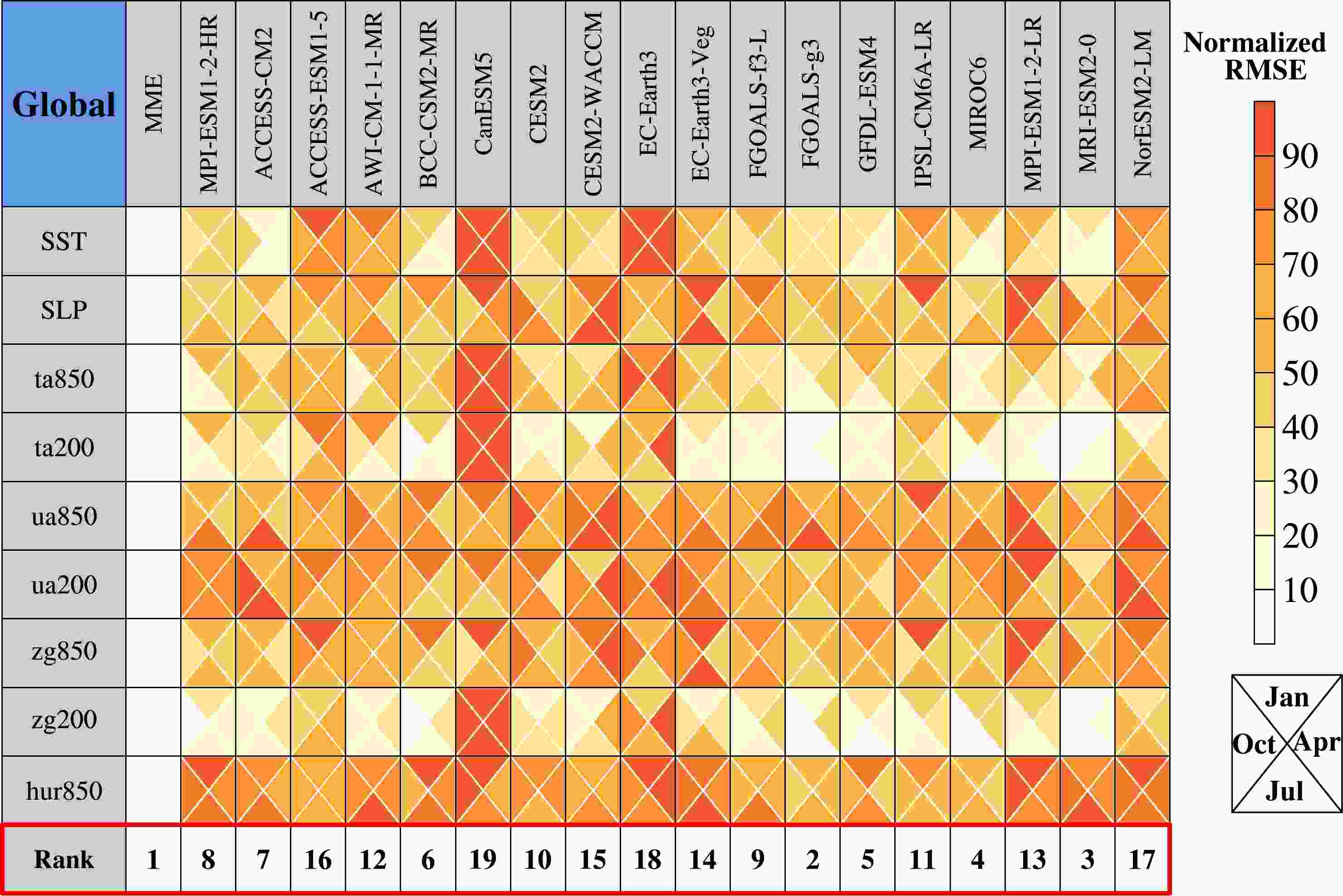
Figure 1. Global mean and normalized RMSE of non-linear trend between individual CMIP6 models or MME with ERA5 reanalysis as a reference. The models are ranked based on the normalized RMSE averaged over all variables and months.
-
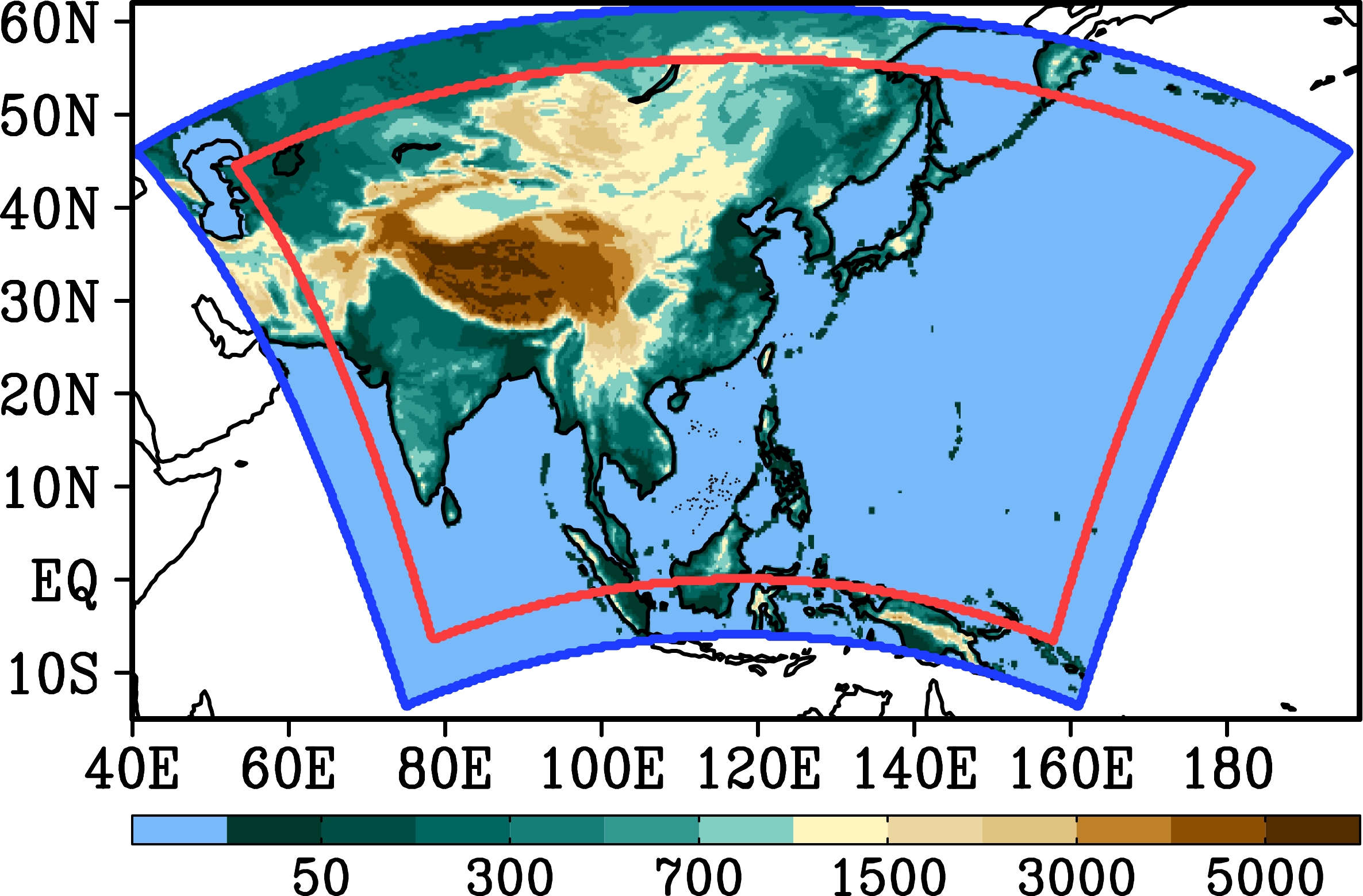
We used the Weather Research and Forecasting (WRF) model with the Advanced Research WRF (ARW) dynamical core version 4.2 (Skamarock et al., 2008). The WRF model was configured at a 25-km grid spacing, which is one of the typical resolutions for CORDEX (COordinated Regional Downscaling EXperiment) models. Our model domain covered most of Asia and the western North Pacific with 33 vertical levels (Fig. 2). Based on the evaluation of multiple parameterization schemes over the East Asian domain, the WRF model was configured with the Kain-Fritsch convective parameterization scheme (Kain, 2004), RRTMG shortwave and longwave radiation schemes (Iacono et al., 2008), the Lin microphysics scheme (Lin et al., 1983), the Noah-MP land surface model (Niu et al., 2011), and the Yonsei University planetary boundary layer scheme (Hong et al., 2006).
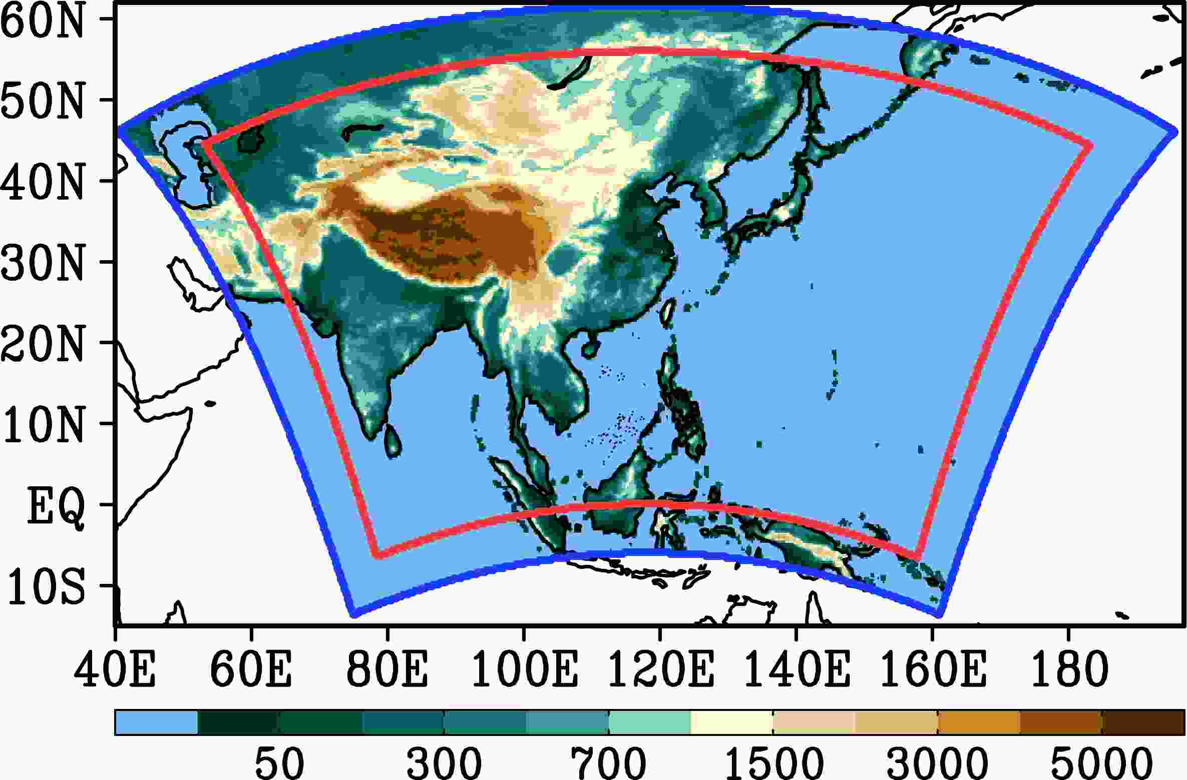
Figure 2. The WRF model domain (shaded area), terrain height (m), and verification region (thick red line excluding 20 grid cells on each side of the WRF domain).
Three WRF simulations were carried out throughout 1980–2014 with the 6-hourly MPI-ESM1-2-HR (WRF_GCM), bias-corrected CMIP6 data (WRF_GCMbc), and the ERA5 (WRF_ERA5) as large-scale forcing data, respectively. The first two years were discarded for spin-up. We compared the WRF_ERA5 with the CRU dataset to validate the performance of the WRF model in simulating the surface air temperature (SAT) and precipitation (Figs. S2 and S3 in the ESM). The results suggest that the WRF model can reasonably reproduce the spatial pattern of climatological mean SAT and precipitation. However, significant errors are still observed. For example, the WRF model overestimated the SAT by 1°C–5°C over most of the Asian continent in summer but underestimated the SAT by 2°C–8°C over China and Southeast Asia in winter. The WRF model overestimated precipitation over East Asia with the maximum errors of approximately 10 mm d–1 to the southeast of the Tibetan Plateau but underestimated precipitation by 2–6 mm d–1 over South Asia in summer. These errors are generally similar to those reported in the previous study (Yu et al., 2020). The WRF_GCM and WRF_GCMbc were validated against the WRF_ERA5 to examine the impact of GCM bias corrections and exclude the impacts of the RCM biases on dynamical downscaling simulations. Assuming that the ERA5 can provide a perfect initial condition, LBCs, and SST, the difference between the WRF_GCM/WRF_GCMbc and the WRF_ERA5 represents the impacts of biases in the SST and LBCs.
-
The amplitude of temporal variation of a scalar variable (M) is measured using standard deviation, as:
where N is the number of years.
$ \overline{M} $ is the climatological mean of Mi for the period 1982–2014. Similarly, we can define the standard deviation of vector winds (Xu et al., 2016) as:where
$\overline u $ and$\overline v $ represent the climatological mean of zonal and meridional components of vector wind, respectively; σv takes both the vector length and vector direction into account, which can measure the amplitude of temporal variation of vector wind.To validate the WRF simulations, we employed the mean error (ME), the root-mean-square error (RMSE), and root-mean-square vector error (RMSVE), which are formulated as follows:
where Mi and Oi are scalar variables derived from the model and observation, respectively. The overbar represents the climatological mean of scalar variables derived from the monthly mean output of the WRF simulation. The indexes N and G are the number of years and grid points, respectively. The RMSVE is the same as the RMSE except for vector fields. The superscripts u and v denote the zonal and meridional components of vector wind, respectively. ME measures the climatological mean difference between the two simulations in each grid cell. The RMSE (RMSVE) summarizes the multiple statistics of a climate model because it is a function of the mean error, pattern correlation, and variance (Xu et al., 2016; Xu and Han, 2020). These statistical metrics were computed within the verification zone as shown in Fig. 2 using the 33-year WRF simulations from 1982 to 2014. We used a Student’s t-test, which takes serial correlation into account, to identify the significance of differences between the two experiments (Zwiers and von Storch, 1995).
-
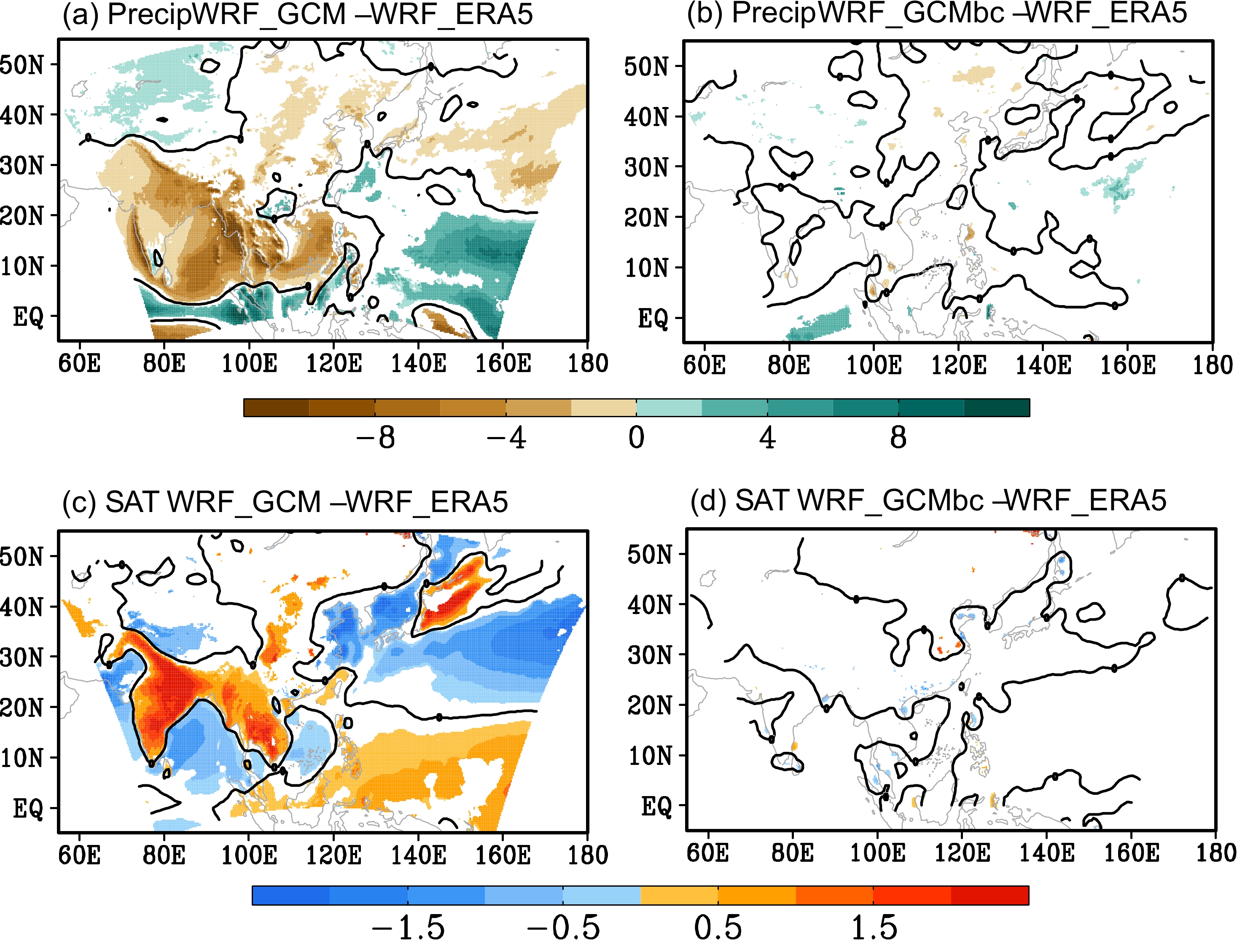
Compared with the WRF_ERA5, the WRF_GCM significantly overestimated (underestimated) precipitation and SAT over the western North Pacific to the south (north) of 20°N (Figs. 3a, c). The error of SST in the large-scale forcing dataset shows a similar spatial pattern as that in the WRF_GCM, which indicates that the errors in precipitation and SAT possibly result from the SST bias over the western North Pacific (figure not shown). A warmer SST leads to higher SAT and more precipitation and vice versa. In contrast, the WRF_GCM significantly underestimated the precipitation, while overestimating the SAT over the Indian and Indochina Peninsula compared with the WRF_ERA5 (Figs. 3a, c). Notably, there is a consistency in the spatial patterns of overestimated SAT and underestimated precipitation over the land area. The decrease in precipitation is accompanied by increased downward solar radiation and a reduction in evapotranspiration from the land surface, which in turn leads to a higher SAT. The errors in downscaled precipitation and SAT are related to the errors in SST and upper-air variables, which will be further addressed in the next section. On the other hand, for the WRF_GCMbc, the errors in precipitation and SAT were significantly minimized for the entire domain (Fig. 3).
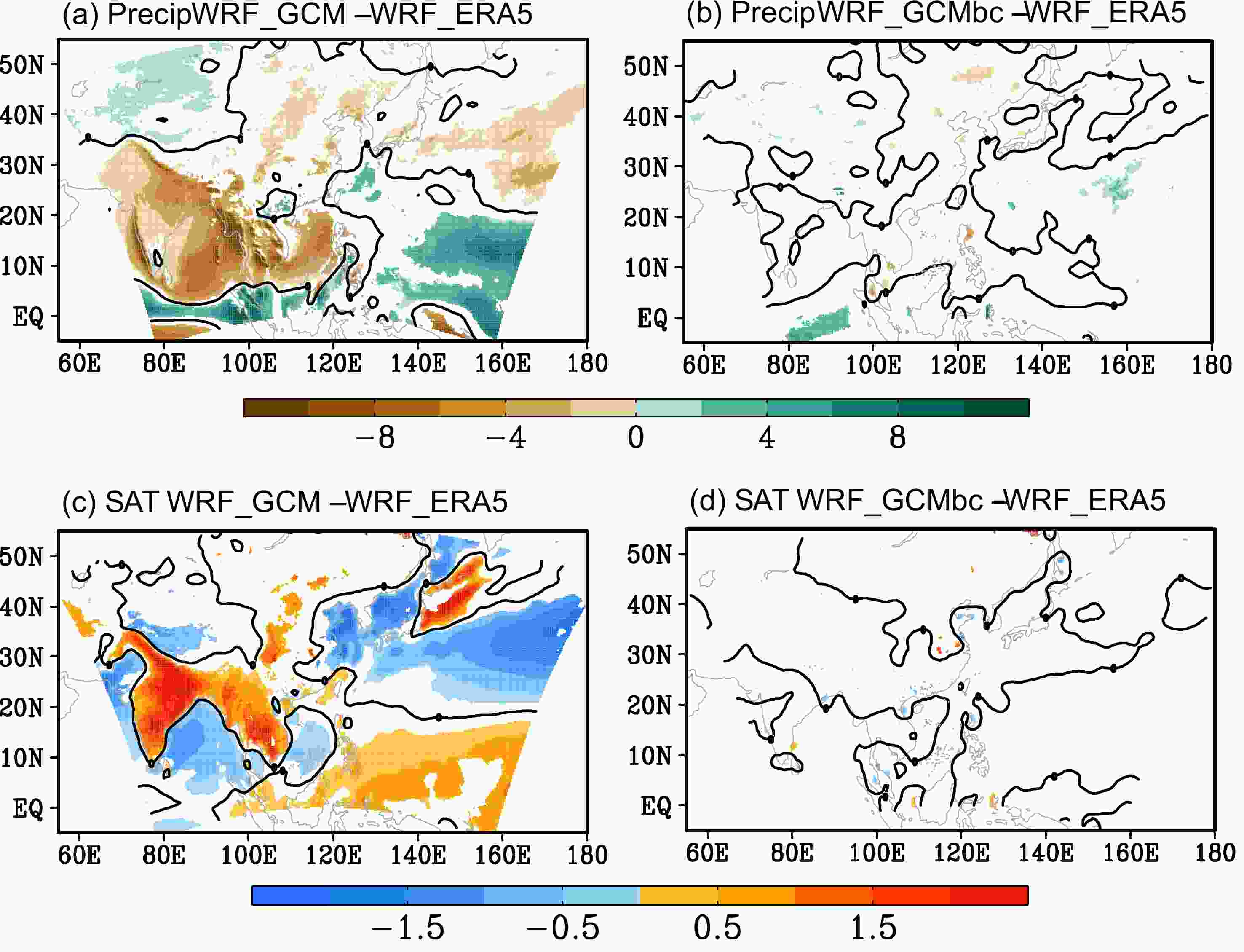
Figure 3. Mean errors of the precipitation (mm d–1) and surface air temperature (°C) in summer during the period 1982–2014. The shaded areas indicate regions where the error exceeds a significance level of 0.05.
In addition to the precipitation and SAT, other surface meteorological variables were also evaluated (Table 1). In comparison to the WRF_GCM, the WRF_GCMbc exhibited much smaller RMSEs in terms of the climatological means of the 2-m specific humidity, snow depth, sensible heat flux, latent heat flux, planetary boundary layer height, and 10-m wind speed. Generally, the RMSEs of the surface variables were reduced by 50%–80%. This improvement was more significant for summer than winter, especially for SAT, snow depth, sensible heat, latent heat, planetary boundary layer height, and 10-m wind speed. For example, the RMSE of SAT is reduced from 0.74°C in the WRF_GCM to 0.19°C in the WRF_GCMbc in summer. In contrast, the RMSE of SAT is reduced from 0.86°C in the WRF_GCM to 0.41°C in the WRF_GCMbc in winter. The errors in SAT primarily occur over mid-high latitudes and the Tibetan Plateau in winter, which is likely related to errors in the snow simulation (Meng et al., 2018).
SAT
(°C)SH2
(g kg–1)Precip
(mm d–1)Snowh
(mm)SHF
(W s–2)LHF
(W s–2)PBLH
(m)Wind10
(m s–1)(a) Climatological mean (WRF_GCM/WRF_GCMbc) Spring 0.87/0.18 0.69/0.13 3.15/0.95 4.46/1.62 6.07/2.23 15.34/5.25 42.49/16.99 0.42/0.14 Summer 0.74/0.19 0.69/0.13 3.37/1.05 2.61/0.70 6.77/1.63 21.94/4.53 53.11/14.65 0.69/0.16 Autumn 0.59/0.17 0.59/0.12 3.25/1.05 2.74/0.95 5.48/2.60 16.99/5.77 40.72/15.64 0.62/0.15 Winter 0.86/0.41 0.74/0.11 3.30/0.52 3.78/1.72 10.2/6.91 20.27/6.58 46.84/23.50 0.50/0.16 (b) Interannual-to-interdecadal standard deviation (WRF_GCM/WRF_GCMbc) Spring 0.34/0.23 0.26/0.11 1.79/1.00 1.76/0.86 3.77/1.96 6.90/3.52 22.36/12.93 0.19/0.08 Summer 0.29/0.13 0.27/0.09 1.95/0.93 1.25/0.54 3.20/1.20 7.01/3.82 20.02/11.12 0.21/0.11 Autumn 0.28/0.11 0.30/0.10 2.06/1.04 1.24/0.72 3.37/2.03 8.32/3.21 20.09/10.44 0.16/0.09 Winter 0.30/0.19 0.17/0.07 1.53/0.68 1.32/0.91 3.38/1.69 6.57/3.03 15.51/10.07 0.15/0.08 (c) Day-to-day variability (WRF_GCM/WRF_GCMbc) Spring 0.13/0.05 0.08/0.04 0.22/0.10 1.39/0.52 1.61/0.66 3.58/1.71 9.28/4.47 0.11/0.07 Summer 0.08/0.05 0.09/0.03 0.27/0.11 0.08/0.03 1.18/0.44 4.50/1.41 8.59/3.94 0.18/0.06 Autumn 0.15/0.05 0.09/0.04 0.28/0.10 0.10/0.05 1.83/0.81 4.92/1.71 10.25/4.41 0.20/0.07 Winter 0.20/0.09 0.09/0.03 0.26/0.06 1.41/0.62 2.71/1.52 4.36/1.67 11.94/5.58 0.13/0.06 SAT: surface air temperature, SH2: 2-m specific humidity, Precip: precipitation, Snowh: snow depth, SHF: sensible heat flux, LHF: latent heat flux, PBLH: planetary boundary layer height, Wind10: 10-m wind speed. Table 1. RMSEs for the climatological mean, interannual-to-interdecadal, and day-to-day variabilities of various variables in different seasons calculated within the verification region illustrated in Fig. 2.
-
We also computed the RMSEs of downscaled upper-air temperature, geopotential height, vector wind, and relative humidity in summer (Fig. S4 in the ESM). The WRF_GCM showed that the largest RMSEs for the air temperature, geopotential height, and vector wind occur in the upper troposphere, while those for relative humidity occur in the mid-troposphere. Compared with the WRF_GCM, the WRF_GCMbc showed much smaller RMSEs of upper-air variables in all vertical levels in summer (Fig. S4 in the ESM). Generally, the RMSEs of downscaled upper-air variables were reduced by approximately 70%–90% due to the GCM bias corrections. Similarly, the WRF_GCMbc also exhibited significant improvement in simulating upper-air variables in other seasons (figure not shown).
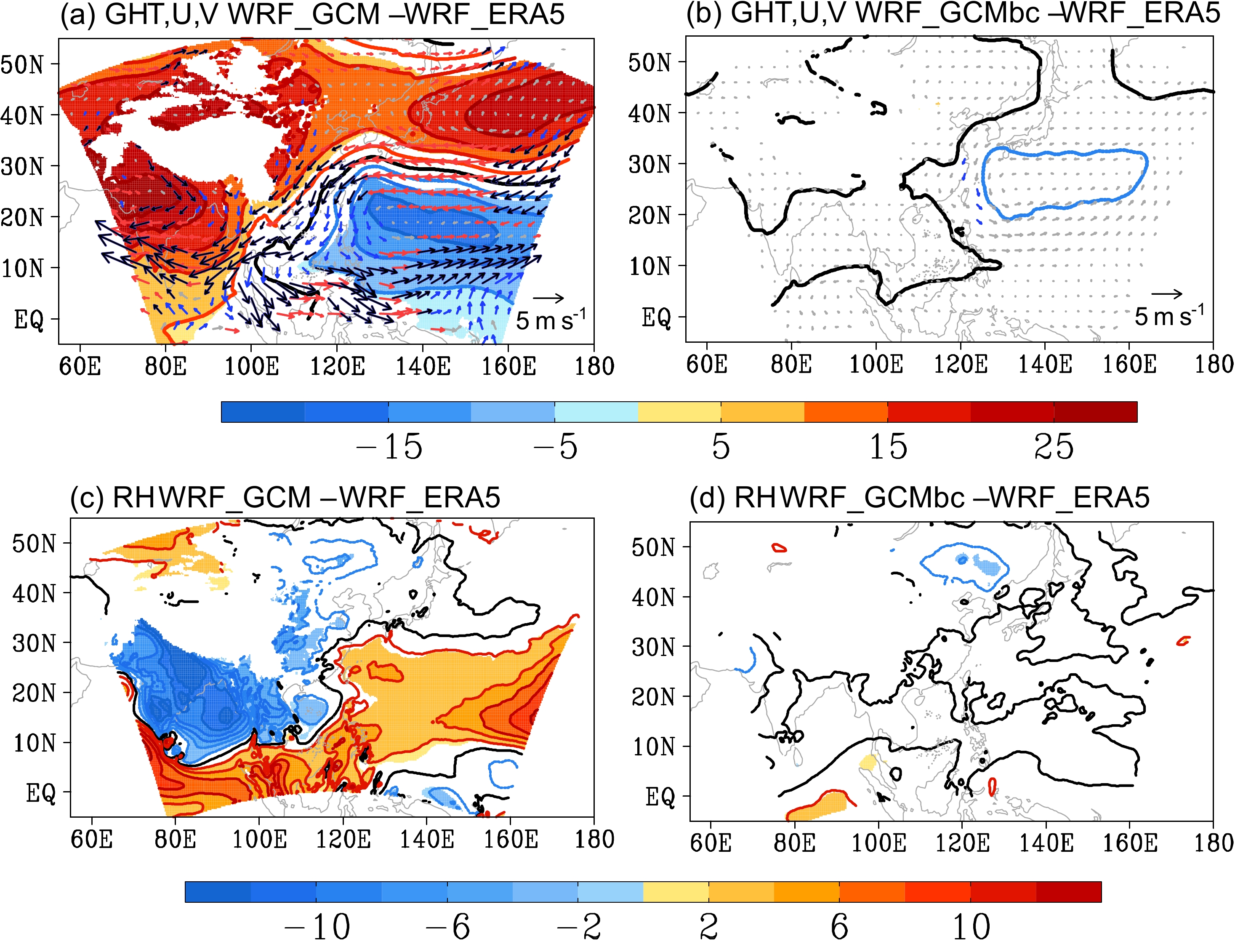
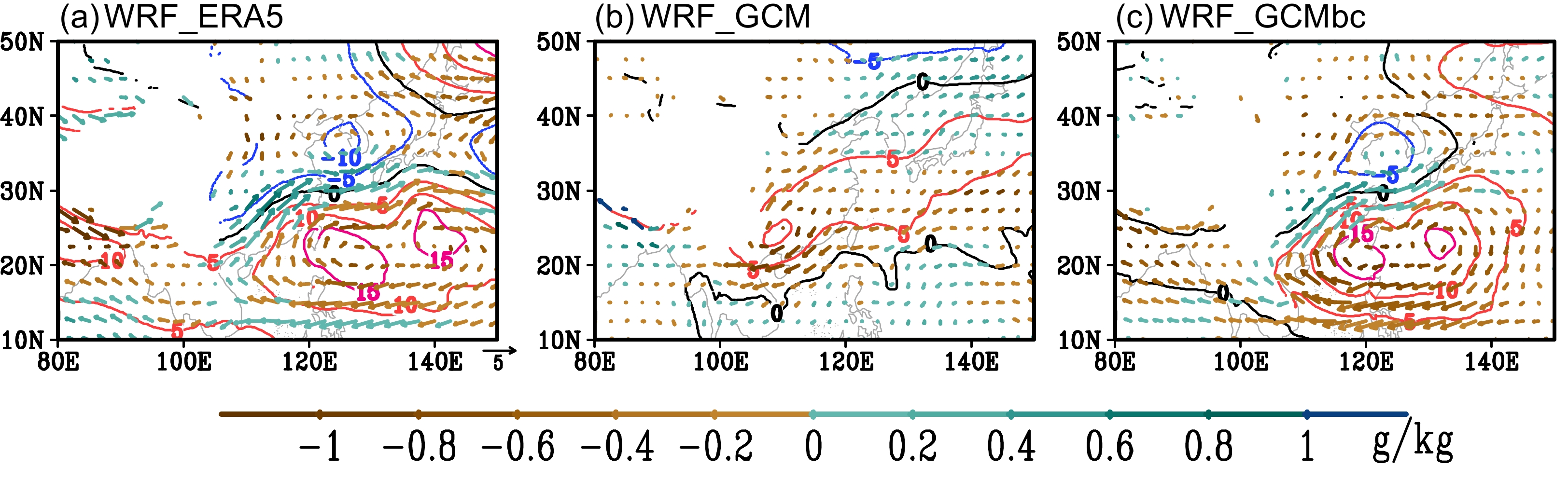
Figure 4 illustrates the spatial pattern of climatological mean errors in 850-hPa geopotential height, vector wind, and relative humidity in summer. Compared with the WRF_ERA5, the WRF_GCM significantly underestimated the geopotential height over the western North Pacific between 5°N and 30°N, while overestimating it across the Asian continent and western North Pacific to the north of 30°N. In association with the geopotential height errors, the 850-hPa vector wind showed a significant cyclonic error in the western North Pacific between 5°N and 30°N and an anticyclonic error around the Tibetan Plateau (Fig. 4a). The anticyclonic error in 850-hPa vector wind and the negative error in relative humidity corresponded to dry and warm errors over India and the Bay of Bengal. Similarly, the cyclonic error and the positive error in relative humidity were associated with an overestimation of precipitation over the western North Pacific between 5°N and 20°N in the WRF_GCM relative to the WRF_ERA5 (Figs. 3a, c and 4a, c). We also noted a spatial consistency in the patterns of errors for both the 850-hPa geopotential height and vector wind between the WRF_GCM and MPI-ESM1-2-HR (figure not shown). This indicates that the errors in the downscaled 850-hPa circulations are largely inherited from the large-scale forcing data. In terms of the simulation of 850-hPa relative humidity, the WRF_GCM also exhibited significant errors relative to the WRF_ERA5, with an overestimation over the western North Pacific and equatorial Indian Ocean and an underestimation over India and the Bay of Bengal (Fig. 4c). Overall, the downscaled circulation, relative humidity, precipitation, and SAT improved significantly due to the GCM bias corrections (Figs. 3 and 4).

Figure 4. Mean errors of 850-hPa geopotential height (gpm), vector wind (m s–1), and relative humidity (g kg–1) in summer (June–July–August) for the period 1982–2014. Shaded areas represent the errors reaching the 0.05 significance level. The red, blue, and black arrows indicate that the zonal wind, meridional wind, or both of them have reached a significance level of 0.05, respectively.
Notably, the GCM bias correction leads to a more significant improvement in dynamical downscaling simulations compared with that presented in Xu and Yang (2012), especially in the lower troposphere. In the previous study, the dynamical downscaling simulations were forced by observed SST data, and the GCM bias corrections were only applied to the upper-air variables (Xu and Yang, 2012). In contrast, the upper-air variables and SST biases were simultaneously corrected in this study. The additional bias corrections to SST lead to a greater improvement in the dynamical downscaling simulations, especially for the lower tropospheric variables.
-
The onset of the SCS summer monsoon generally occurs around mid-May, which signifies the beginning of the East Asian summer monsoon (Wang et al., 2004). Following Wang et al. (2004), the South China Sea (SCS) monsoon index, uSCS, is defined as the 850-hPa zonal wind averaged over the central SCS (5°–15°N, 110°–120°E). The climatological mean uSCS shows an abrupt seasonal transition from easterly to westerly around mid-May associated with the onset of SCS summer monsoon. The dynamical downscaling simulations were able to reasonably capture the annual cycle of uSCS (Fig. S5 in the ESM). The climatological mean uSCS showed a transition from easterly to westerly around early May in the WRF_ERA5 and WRF_GCMbc. In contrast, the transition occurred in mid-May in the WRF_GCM. The transition from westerly to easterly winds became evident in mid-October in all three WRF simulations. The uSCS derived from the large-scale forcing data (i.e., the ERA5 reanalysis, raw GCM, and the bias-corrected CMIP6 data) showed similar annual cycles as those in the WRF simulations (figure not shown). The only exception was noted for the transition date from easterly to westerly, which occurred almost 10 days later than that in the WRF simulations (Fig. S5 in the ESM). This indicates that the downscaled annual cycle of the SCS monsoon circulation is strongly affected by the large-scale forcing data. However, the WRF simulations tended to generate an earlier onset of westerly flow by approximately 10 days compared to the corresponding large-scale forcing data, which can be attributed to the WRF model bias.
-
In addition to climatological means, temporal variability is also of great importance in the future projection of regional climate and its impacts. Here, the interannual-to-interdecadal variability is measured by the standard deviation of a seasonal mean scalar or vector variable over the period 1982–2014 (Eqs. 2 and 3). Compared with the WRF_ERA5, the WRF_GCM significantly underestimated the interannual-to-interdecadal variability of precipitation over India, the Bay of Bengal, and the South China Sea. In contrast, it overestimated the precipitation variability over the western North Pacific to the south of 20°N (Figs. S6a, b in the ESM). Notably, the spatial patterns of the errors in precipitation variability were consistent with those found for the climatological mean. The errors in precipitation variability were significantly reduced in the WRF_GCMbc. For example, the RMSE of summer precipitation variability was reduced from 1.95 mm d–1 in the WRF_GCM to 0.93 mm d–1 in the WRF_GCMbc (Table 1). Compared with the WRF_ERA5, the WRF_GCM underestimated the interannual-to-interdecadal variance of summer SAT in northwestern India and eastern China while overestimating it over the Bay of Bengal, Indochina Peninsula, and the western North Pacific to the south of 30°N. The errors in the interannual-to-interdecadal variance of downscaled SAT were also greatly reduced in the WRF_GCMbc due to the GCM bias correction (Figs. S6c, d in the ESM).
Similar to precipitation and SAT, other surface variables also exhibited significant improvements in their interannual-to-interdecadal variability in the WRF_GCMbc relative to the WRF_GCM with a reduction of almost 30%–60% in RMSEs (Table 1). Among these surface variables, 2-m specific humidity showed the most pronounced improvement with a decrease in the RMSE by roughly 60%. Overall, the improvement in the downscaled interannual-to-interdecadal variability was relatively small compared with that of the climatological means.
-
The GCM bias correction significantly improved the interannual-to-interdecadal variability of upper air temperature, geopotential height, vector wind, and relative humidity at all vertical levels in summer (Fig. S7 in the ESM) as well as in other seasons (figure not shown). The RMSEs in the interannual-to-interdecadal variability were reduced by 20%–70%. Note that this improvement was smaller than that in climatological means (Figs. S4 and S7 in the ESM). This indicates that it is more challenging to improve downscaled temporal variability than the climatological means by correcting the GCM biases.
Compared with the WRF_ERA5, the WRF_GCM significantly underestimated the interannual-to-interdecadal variability of the 850-hPa geopotential height over the Eastern China-East China Sea and conversely overestimated it over the Maritime Continent and western North Pacific to the east of 140°E (Fig. S8a in the ESM). This suggests that the western North Pacific subtropical high (WNPSH) exhibited a weaker interannual-to-interdecadal variability over East Asia to the south of 40°N in the WRF_GCM than in the WRF_ERA5. In this region, the 850-hPa vector wind also showed a weaker interannual-to-interdecadal variability over eastern China and the South China Sea, which may be linked to the reduced summer precipitation variability in the WRF_GCM (Figs. S6a and S8c in the ESM). Conversely, the WRF_GCM overestimated the vector wind variability over the western North Pacific to the south of 20°N where it also showed an overestimation of precipitation variability relative to the WRF_ERA5. It appears that the variability of the 850-hPa vector wind can partially account for the precipitation variability. In the WRF_GCMbc, the errors in the interannual-to-interdecadal variability of the geopotential height and vector wind were largely removed due to the GCM bias corrections. Consequently, the variability of downscaled precipitation was improved in the WRF_GCMbc.
-
The onset of SCS summer monsoon shows considerable year-to-year variability (Wu and Wang, 2001; Jiang and Zhu, 2021). To examine the temporal variability of the SCS summer monsoon, we defined the onset date of the SCS summer monsoon as the first day after 25 April, where the 5-day running mean of uSCS is greater than 1 m·s-1 and persists for at least 15 days. The variance of SCS summer monsoon onset date was 11.9, 10.6, and 12.6 days in the WRF_ERA5, WRF_GCM, and WRF_GCMbc, respectively (Fig. S9 in the ESM). Clearly, compared with the WRF_GCM, the WRF_GCMbc generated an SCS summer monsoon variability closer to that in the WRF_ERA5. Moreover, both the WRF_GCMbc and WRF_ERA5 showed a clear decline in the onset date of SCS summer monsoon over the period 1982–2014, which was not evident in the WRF_GCM. As discussed in section 2.2, the MME generally shows a more consistent non-linear trend with the ERA5, relative to individual CMIP6 models, which likely helps improve the long-term trend of onset date of the downscaled SCS summer monsoon.
-
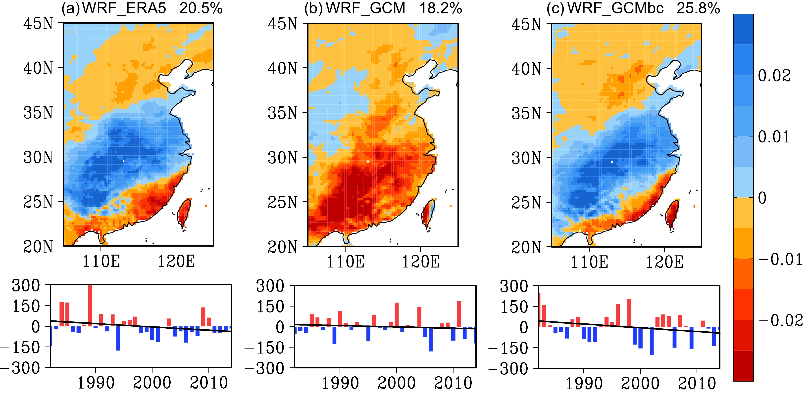
It is known that the leading mode of the Empirical Orthogonal Function (EOF) for the observed summer precipitation shows a dry-wet-dry pattern over the North China-Yangtze River Basin-South China at interannual to interdecadal time scales (Ding et al., 2008). Previous studies suggested that both internal climate variability and external forcing contribute to the precipitation anomalous mode (Yang et al., 2017; Huang et al., 2023). The WRF_ERA5 can reasonably reproduce the tri-pole pattern (–, +, –) of the observed summer precipitation anomaly, characterized by a positive precipitation anomaly over the Yangtze River basin and a negative precipitation anomaly over North China and South China (Fig. 5a). However, the WRF_GCM showed a monopole pattern over eastern China, instead (Fig. 5b). This indicates that summer precipitation varies homogeneously over eastern China in the WRF_GCM. In contrast, the WRF_GCMbc successfully reproduced the tri-pole pattern of summer precipitation anomaly due to the GCM bias corrections (Fig. 5c). In addition to the first EOF mode, the second and third EOF modes in the WRF_GCMbc were also more consistent with those in the WRF_ERA5 relative to the WRF_GCM (Table S1 in the ESM). The first three EOF modes accounted for 52.3%, 43.1%, and 51.4% of the total variance in the WRF_ERA5, WRF_GCM, and WRF_GCMbc, respectively. Note that the WRF_GCMbc well captured the declining trend of the time series of the leading EOF, which is likely due to the improved long-term trend in the MME relative to individual CMIP6 models (Figs. 5a, c and Fig. S1 in the ESM).

Figure 5. Leading EOF mode, PC time series of summer precipitation anomaly (mm d–1, bars), and its trend (thick black line) derived from the WRF_ERA5, ERA_GCM, and WRF_GCMbc, respectively. The variance explained is shown on the top of each panel.
As discussed in section 3.3, the interannual variability of precipitation is related to that of the atmospheric circulation. Therefore, we computed the difference of the 850-hPa geopotential height, vector wind, and moisture between the positive- and negative-phase years of the leading EOF time series. The positive (negative) phase years were defined as the time series of an EOF greater (smaller) than a 0.5 (–0.5) standard deviation. In the positive-phase years, the 850-hPa geopotential height showed a positive (negative) anomaly to the south (north) of 30°N, indicating a southward shift of the WNPSH in the WRF_ERA5 (Fig. 6a). Correspondingly, the 850-hPa circulation revealed an anticyclonic (cyclonic) anomaly to the south (north) of 30°N in the positive-phase years and corresponded to a dry anomaly over South China (Figs. 5a, 6a). The Yangtze River basin was dominated by a southwesterly anomaly, which may bring abundant moisture and a wet anomaly. The southward shift of WNPSH hiders the northward transfer of moisture and results in a dry anomaly over North China (Fig. 6a). The spatial patterns of the 850-hPa geopotential height and vector wind anomalies in the WRF_GCMbc were consistent with those in the WRF_ERA5. Consequently, the WRF_GCMbc well captured the leading EOF of summer precipitation anomaly. In contrast, the WRF_GCM generated a positive 850-hPa geopotential height anomaly over East Asia between 20°N and 40°N in the positive-phase years relative to the negative-phase years (Fig. 6b). In turn, the enhanced WNPSH causes a dry anomaly over eastern China and vice versa.
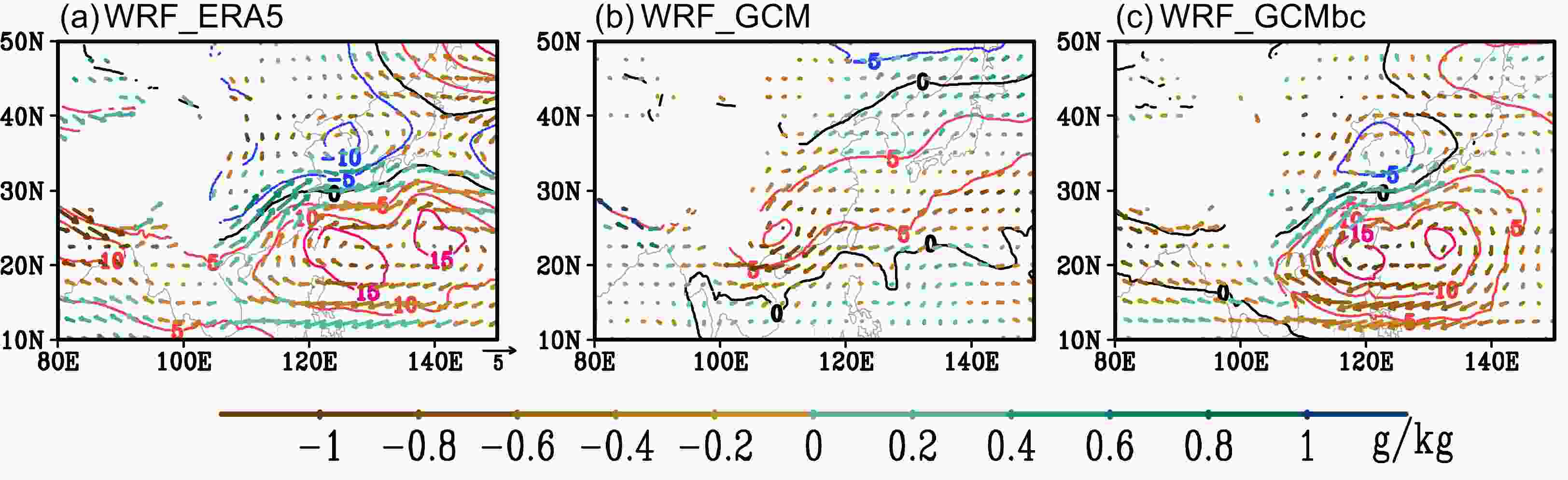
Figure 6. Differences in the 850-hPa geopotential height (m2 s–2), vector wind (m s–1), and moisture (g kg–1) between the positive and negative phase years. A positive (negative) year is defined by the time series of the first EOF (Fig. 5) greater (smaller) than its 0.5 (–0.5) standard deviation. The contour and its color represent geopotential height and specific humidity, respectively.
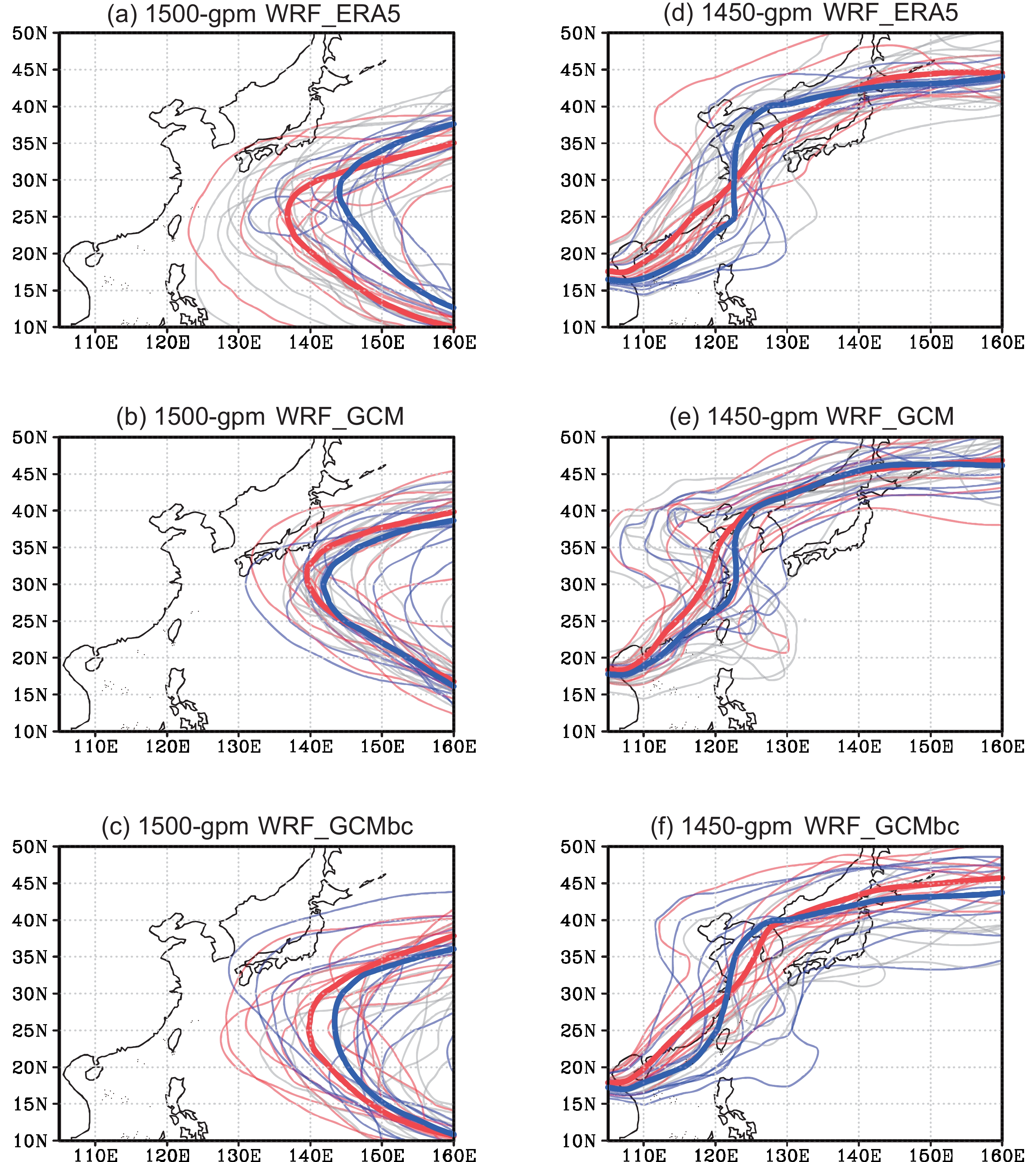
Figure 7 further illustrates the contours of 1500 geopotential meters (gpm) and 1450 gpm of the summer WNPSH in the WRF_ERA5, WRF_GCM, and WRF_GCMbc throughout 1982–2014. The 1500-gpm contour can roughly illustrate the location of the WNPSH. Based on the geostrophic balance between the geopotential height and wind, wind generally flows along the isobars. Thus, the 1450-gpm contour can roughly represent the 850-hPa prevailing wind direction over eastern China. In the WRF_ERA5, the WNPSH extended southwestward in the positive-phase years, leading to a positive (negative) geopotential height anomaly to the south (north) of 30°N (Figs. 6a and 7a). The prevailing wind flows from the Indo-China peninsula to the East China Sea as indicated by the 1450-gpm contour in the positive-phase years, which brings more precipitation to the Yangtze River basin and less precipitation to South China and North China (Figs. 5a, 6a, and the red lines in Fig. 7d). In the negative-phase years, the WNPSH extended northward and the 1450-gpm contour showed a south-north orientation, which can bring more moisture and precipitation to North China (blue lines in Figs. 7a, d). However, the WRF_GCM demonstrated less skill in capturing the location of the WNPSH ridge, which was characterized by a roughly 5-degree northward migration relative to that in the WRF_ERA5 (Figs. 7a, b). The 1450-gpm contour extended westward in the positive-phase years relative to the negative-phase years over eastern China between 20°N and 40°N, inducing a monopole pattern of summer precipitation anomaly (Figs. 5b and 7e). Notably, the error in the location of the WNSPH ridge was greatly reduced in the WRF_GCMbc due to the GCM bias corrections (Figs. 7a–c). Moreover, the 1450-gpm contours revealed a very similar spatial pattern between 20°N and 40°N as that in the WRF_ERA5, i.e., a southwest-northeast orientation in the positive-phase years and a south-north orientation in the negative phase years (Figs. 7d, f). This spatial pattern of geopotential height is crucial for generating the leading EOF pattern of the observed summer precipitation anomaly over eastern China.
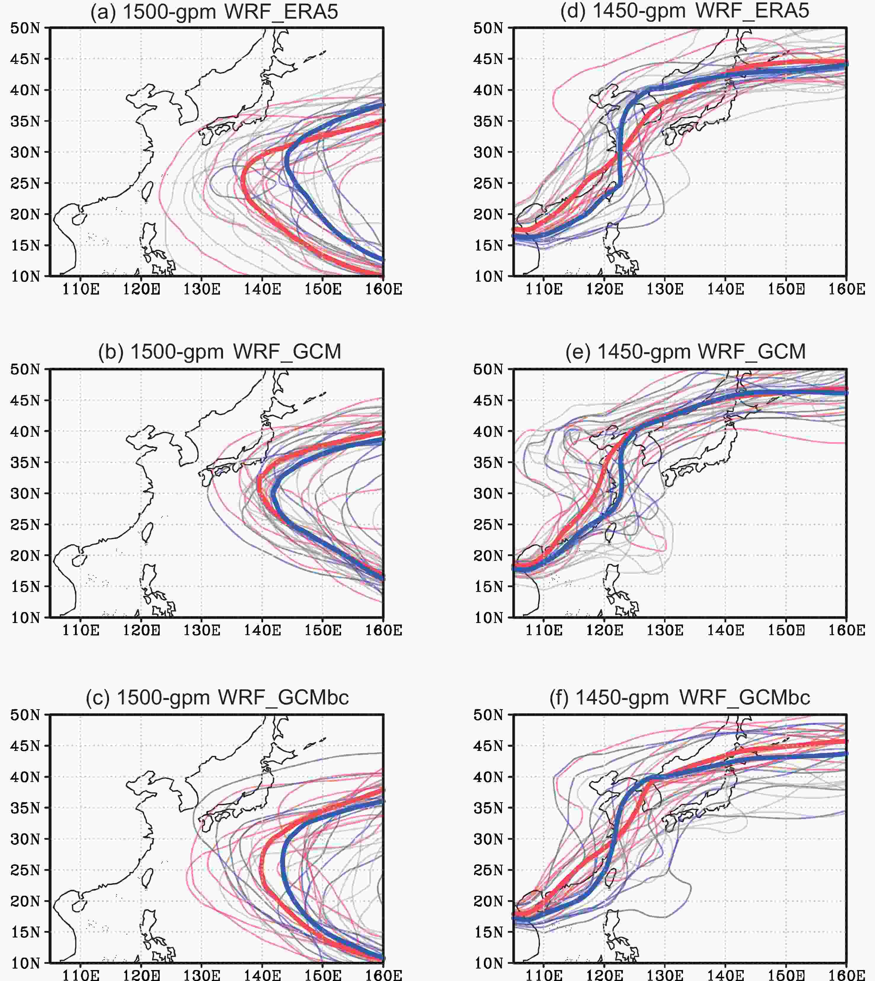
Figure 7. The 1500-gpm and 1450-gpm contours of geopotential heights in the (a, d) WRF_ERA5, (b, e) WRF_GCM, and (c, f) WRF_GCMbc for positive-phase (red line), negative-phase (blue line), and normal years (grey line) from 1982–2014. The thick red and blue contours represent the geopotential height averaged over the positive-phase and negative-phase years, respectively. The positive (negative) years are the same as in Fig. 6.
-
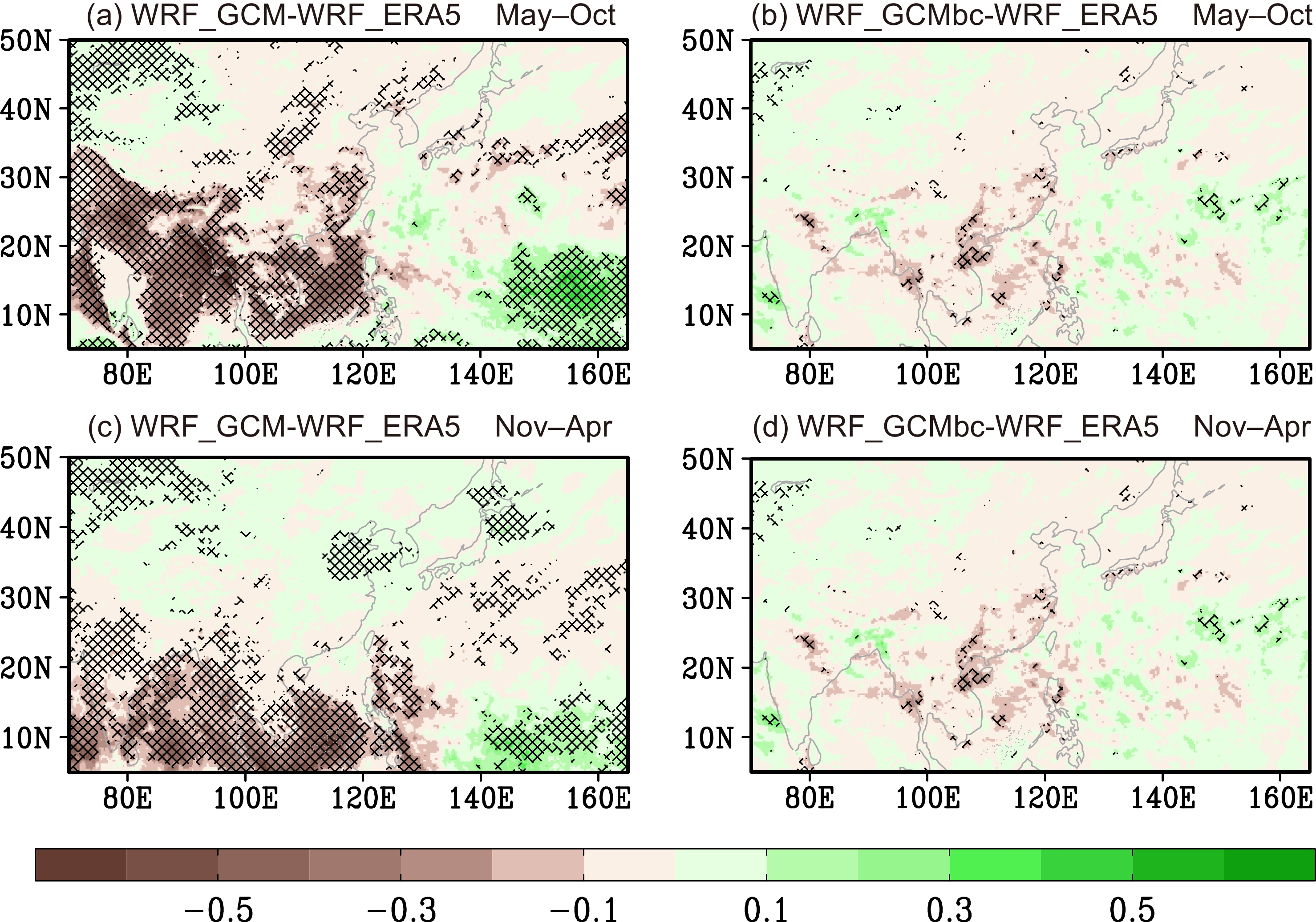
To evaluate the downscaled intraseasonal oscillation (ISO), we calculated the variance of the 20–100-day filtered precipitation averaged in the summer and winter half of the year (Fig. 8). Compared with the WRF_ERA5, the WRF_GCM significantly underestimated the ISO strength over South and Southeast Asia, while overestimating it over the western North Pacific (5°–20°N, 140°–165°E) in the summer half year (Fig. 8a). In the WRF_GCMbc, the mean error of the ISO strength was greatly reduced compared to the WRF_GCM, suggesting that the GCM bias correction can significantly improve the downscaled ISO strength over the Asia-western North Pacific domain (Figs. 8a, b). Moreover, the variance of 20–100-day filtered 850-hPa zonal wind showed similar errors to those of precipitation either in the WRF_GCM or its large-scale forcing data. These errors were greatly reduced after GCM bias correction (figures not shown). This indicates that the RCM simulation driven by the bias-corrected CMIP6 data can well capture the ISO intensity of downscaled precipitation. Similar to the summer half-year, GCM bias correction can also significantly improve the downscaled ISO in the winter half-year (Figs. 8c, d).
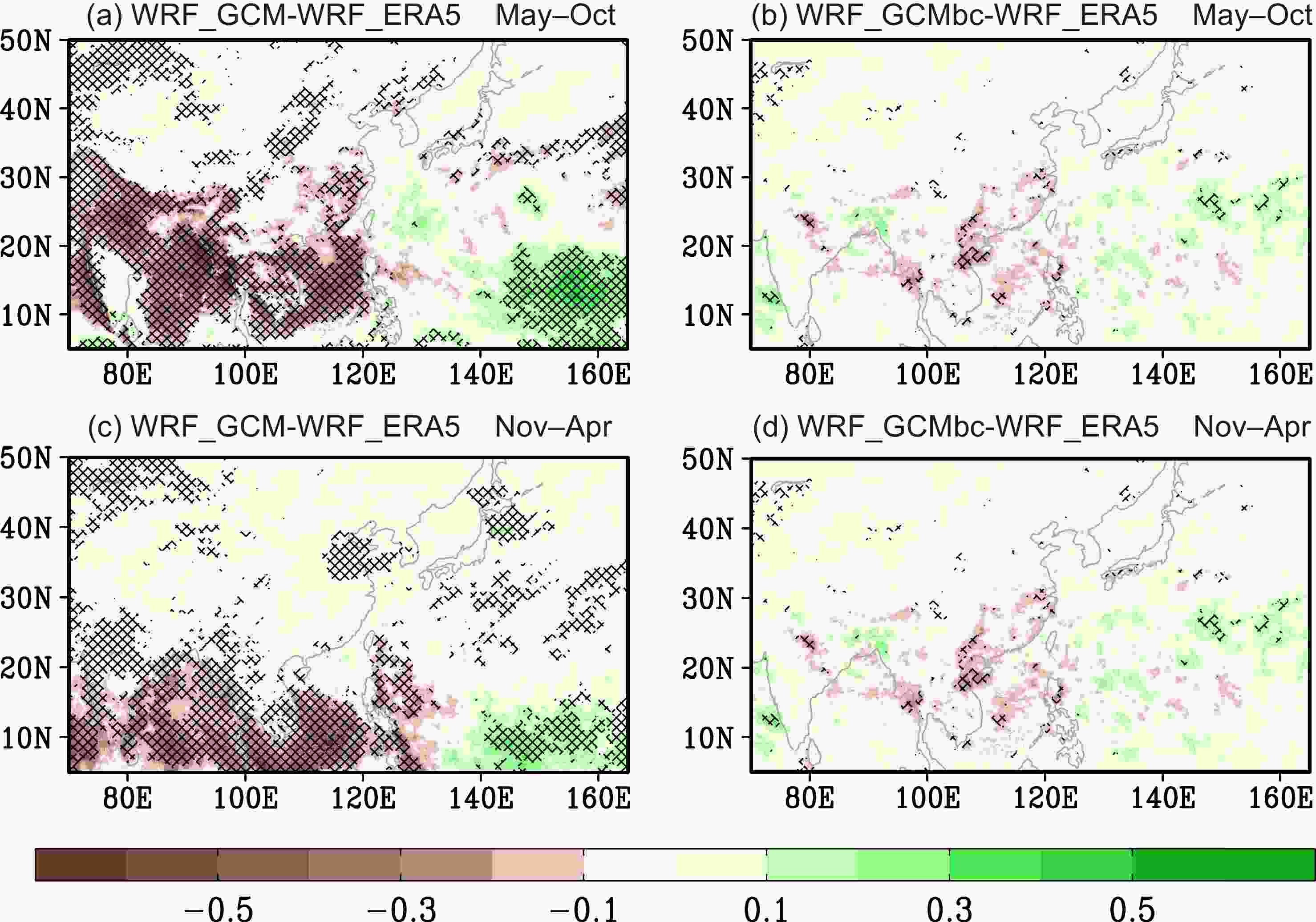
Figure 8. Mean errors of the standard deviation of the 20–100-day filtered intraseasonal precipitation (mm d–1) for the summer (May–October) and winter (November–April) half-year averaged over the period 1982–2014. The hatched area indicates that the difference reached the significance level of 0.05.
-
The day-to-day (DTD) temperature variability, defined as the mean absolute difference of the surface air temperature between two adjacent days, is one of the important factors that likely affect human health (Liu et al., 2020; Xu et al., 2020). Compared with the WRF_ERA5, the WRF_GCM significantly overestimated the DTD temperature variability by 0.1°C–0.4°C across the Asian continent, while underestimating it by 0.1°C–0.3°C over the western North Pacific between 20°N and 40°N (Fig. 9a). These errors in the downscaled DTD temperature variability were greatly reduced in the WRF_GCMbc due to the GCM bias correction (Figs. 9a, b).

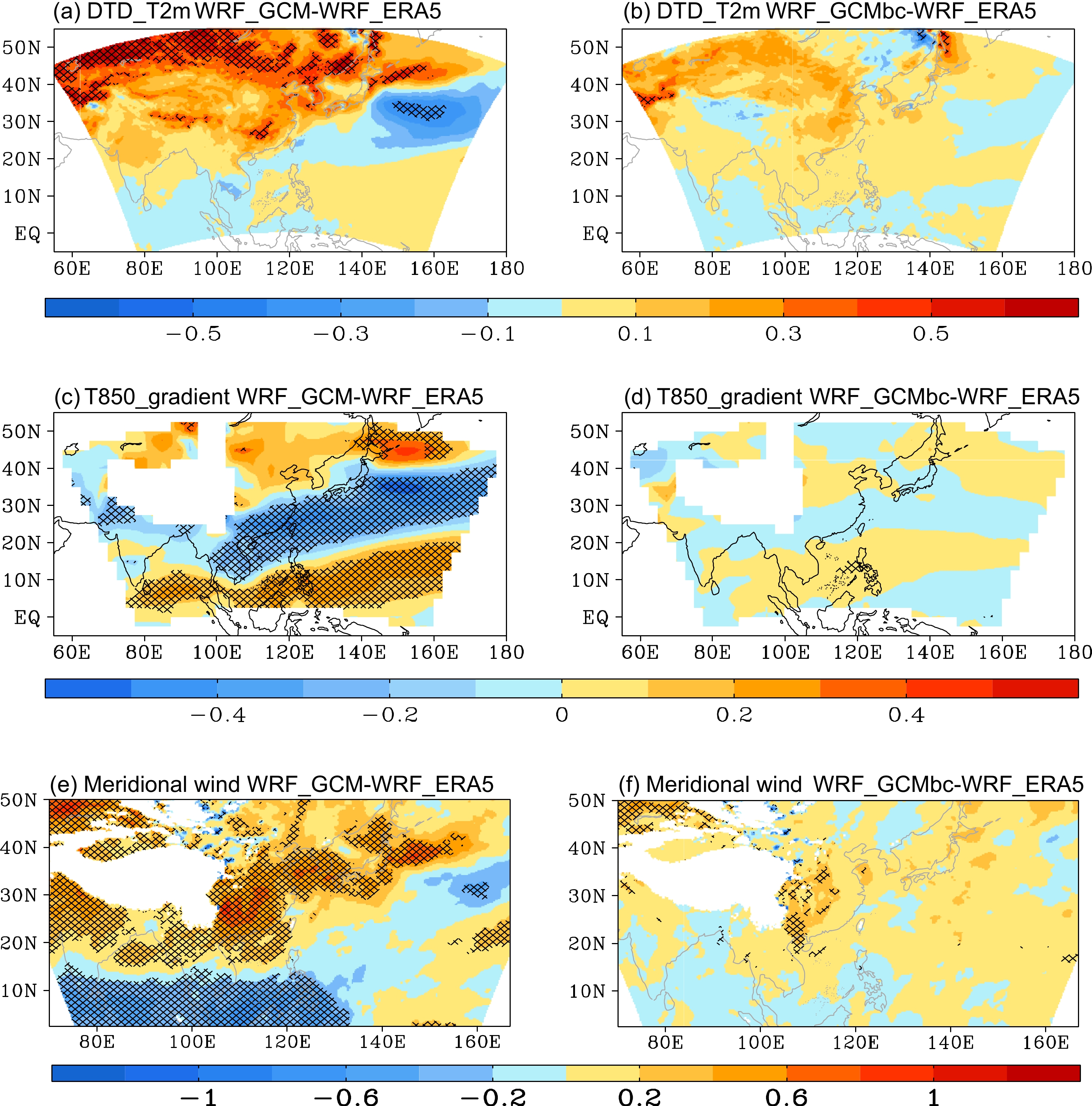
Figure 9. Mean error of day-to-day variability of 2-m air temperature (units: °C), 850-hPa meridional wind and climatological mean meridional temperature gradient [units: °C (100 km)–1] at 850 hPa in winter (December–January–February) during the period 1982–2014. The mean errors in (c) and (d) were calculated with the absolute value of temperature gradient derived from the WRF_GCM (WRF_GCMbc) and WRF_ERA5. The hatched area indicates that the error reached a significance level of 0.05.
It is known that temperature advection is one of the key factors that affect DTD temperature variability (e.g., Xu et al., 2020). To identify the source of error in DTD temperature variability, we calculated the climatological mean meridional temperature gradient and DTD variability of the 850-hPa meridional wind (Figs. 9c–f). Compared with the WRF_ERA5, the WRF_GCM overestimated the temperature gradient over the Asian continent to the north of 35°N, which is favorable for increasing the temperature advection and DTD temperature variability there. Similarly, the reduced temperature gradient over the western North Pacific corresponded to a decrease in DTD temperature variability between 20°N and 40°N (Figs. 9a, c). However, the increase in DTD temperature variability over southern China and northern India may be attributed to enhanced DTD variability of the 850-hPa meridional wind rather than the temperature gradient (Figs. 9a, c, e). The GCM bias correction significantly reduced the errors in the downscaled 850-hPa temperature gradient and the daily 850-hPa meridional wind variability, leading to an improvement in DTD temperature variability (Fig. 9).
-
It is well known that the errors in the large-scaling forcing data can propagate into an RCM through the lateral boundary conditions and degraded RCM simulations. This is often referred to as the “garbage in, garbage out” issue (Giorgi and Mearns, 1999; Hall, 2014). In this study, our dynamical downscaling simulation used bias-corrected GCM data to reduce the “garbage” in the large-scale forcing data (Xu et al., 2021).
Compared with previous studies, the bias-corrected GCM data was constructed with the state-of-the-art ERA5 reanalysis and CMIP6 data. It has not yet been assessed as to what extent the bias-corrected CMIP6 data can improve the dynamical downscaling simulation over the Asia-western North Pacific. In this study, we carried out a comprehensive evaluation of the long-term RCM simulations from various aspects. Our results indicate that the RCM simulation with bias-corrected GCM data shows a greatly improved performance in terms of multiple variables at different vertical levels and different time scales, e.g., the climatological mean, annual cycle, interannual-to-interdecadal, intraseasonal, and day-to-day variabilities. The RMSEs of the climatological means were reduced by 70%–90% for the upper-air variables (e.g., air temperature, geopotential height, vector wind, and relative humidity) and 50%–80% for the surface variables (e.g., SAT, precipitation, sensible heat flux, and 10-m wind speed). The RMSEs of temporal variances were reduced by 20%–70% for the downscaled upper-air and surface variables due to the GCM bias corrections. Moreover, we also identify significant improvement in the downscaled intra-seasonal variability of precipitation and day-to-day temperature variability over the entire RCM domain.
More interestingly, the dynamical downscaling simulation with GCM bias corrections can significantly improve the leading EOF mode of summer precipitation over eastern China, although we did not correct the EOF mode of large-scale forcing data. The GCM bias correction generates a more accurate location of WNPSH and its associated atmospheric circulation, which in turn improves the dynamics of the RCM and downscaled precipitation variability. This is a particular advantage of applying GCM bias corrections prior to dynamical downscaling simulations, as opposed to using a bias correction for post-processing only, and is considered to be of great importance. Based on the findings presented in this paper, we anticipate that the dynamical downscaling approach can also yield improved simulations in other regions across the globe. Given the substantial improvement in the surface and upper-air variables, the utilization of bias-corrected CMIP6 data in dynamical downscaling is expected to generate improved projections of regional climate, air quality, hydrology, agriculture, wind power, and other related fields.
Note that we only evaluated the dynamical downscaling simulation with one set of bias-corrected CMIP6 data in this study. Thus, it is impossible to measure the model uncertainty. However, a proper estimation of uncertainty is crucial for future climate projection and risk assessment (van Oldenborgh et al., 2013; Shepherd, 2014). To measure the model uncertainty, one can construct multiple bias-corrected data using various CMIP6 models and carry out ensemble downscaling simulations. Alternatively, using the dynamical downscaling simulation and multiple CMIP6 model data, one can further employ a hybrid dynamical-statistical downscaling approach to generate ensemble downscaling data (Walton et al., 2015). It is interesting to further compare the ensemble downscaling simulations with and without GCM bias correction. Such a comparison would help to evaluate the potential impacts of GCM bias correction on the uncertainty range within an ensemble dynamical downscaling projection.
Acknowledgements. The study was supported jointly by the National Natural Science Foundation of China (Grant No. 42075170), the National Key Research and Development Program of China (2022YFF0802503), the Jiangsu Collaborative Innovation Center for Climate Change, and a Chinese University Direct Grant (Grant No. 4053331). This study was also supported by the National Key Scientific and Technological Infrastructure project “Earth System Numerical Simulator Facility” (EarthLab).
Electronic supplementary material: Supplementary material is available in the online version of this article at
https://doi.org/10.1007/s00376-023-3101-y .
| SAT (°C) |
SH2 (g kg–1) |
Precip (mm d–1) |
Snowh (mm) |
SHF (W s–2) |
LHF (W s–2) |
PBLH (m) |
Wind10 (m s–1) |
|
| (a) Climatological mean (WRF_GCM/WRF_GCMbc) | ||||||||
| Spring | 0.87/0.18 | 0.69/0.13 | 3.15/0.95 | 4.46/1.62 | 6.07/2.23 | 15.34/5.25 | 42.49/16.99 | 0.42/0.14 |
| Summer | 0.74/0.19 | 0.69/0.13 | 3.37/1.05 | 2.61/0.70 | 6.77/1.63 | 21.94/4.53 | 53.11/14.65 | 0.69/0.16 |
| Autumn | 0.59/0.17 | 0.59/0.12 | 3.25/1.05 | 2.74/0.95 | 5.48/2.60 | 16.99/5.77 | 40.72/15.64 | 0.62/0.15 |
| Winter | 0.86/0.41 | 0.74/0.11 | 3.30/0.52 | 3.78/1.72 | 10.2/6.91 | 20.27/6.58 | 46.84/23.50 | 0.50/0.16 |
| (b) Interannual-to-interdecadal standard deviation (WRF_GCM/WRF_GCMbc) | ||||||||
| Spring | 0.34/0.23 | 0.26/0.11 | 1.79/1.00 | 1.76/0.86 | 3.77/1.96 | 6.90/3.52 | 22.36/12.93 | 0.19/0.08 |
| Summer | 0.29/0.13 | 0.27/0.09 | 1.95/0.93 | 1.25/0.54 | 3.20/1.20 | 7.01/3.82 | 20.02/11.12 | 0.21/0.11 |
| Autumn | 0.28/0.11 | 0.30/0.10 | 2.06/1.04 | 1.24/0.72 | 3.37/2.03 | 8.32/3.21 | 20.09/10.44 | 0.16/0.09 |
| Winter | 0.30/0.19 | 0.17/0.07 | 1.53/0.68 | 1.32/0.91 | 3.38/1.69 | 6.57/3.03 | 15.51/10.07 | 0.15/0.08 |
| (c) Day-to-day variability (WRF_GCM/WRF_GCMbc) | ||||||||
| Spring | 0.13/0.05 | 0.08/0.04 | 0.22/0.10 | 1.39/0.52 | 1.61/0.66 | 3.58/1.71 | 9.28/4.47 | 0.11/0.07 |
| Summer | 0.08/0.05 | 0.09/0.03 | 0.27/0.11 | 0.08/0.03 | 1.18/0.44 | 4.50/1.41 | 8.59/3.94 | 0.18/0.06 |
| Autumn | 0.15/0.05 | 0.09/0.04 | 0.28/0.10 | 0.10/0.05 | 1.83/0.81 | 4.92/1.71 | 10.25/4.41 | 0.20/0.07 |
| Winter | 0.20/0.09 | 0.09/0.03 | 0.26/0.06 | 1.41/0.62 | 2.71/1.52 | 4.36/1.67 | 11.94/5.58 | 0.13/0.06 |
| SAT: surface air temperature, SH2: 2-m specific humidity, Precip: precipitation, Snowh: snow depth, SHF: sensible heat flux, LHF: latent heat flux, PBLH: planetary boundary layer height, Wind10: 10-m wind speed. | ||||||||


 AAS Website
 AAS WeChat