U-Net Models for Representing Wind Stress Anomalies over the Tropical Pacific and Their Integrations with an Intermediate Coupled Model for ENSO Studies

El Niño-Southern Oscillation (ENSO) is the most predominant interannual climate variability over the tropical Pacific (Diaz et al., 2001; Timmermann et al., 2018; Gao et al., 2022, 2023). As a periodically oscillatory climate signal originating from coupled ocean-atmosphere interactions in the tropical Pacific, ENSO profoundly influences the evolution of sea surface temperature (SST), sea surface wind, and the thermocline in the central-eastern equatorial Pacific (Bjerknes, 1969; Zhang et al., 1998, 2020; Wang, 2019). Consequently, the simulation and prediction of ENSO events are active research areas in physical oceanography and meteorology.

To date, many sophisticated dynamical and statistical models with different degrees of complexity have been developed to simulate and predict ENSO events, including intermediate coupled models (ICMs; Hirst, 1986; Zebiak and Cane, 1987; Zhang et al., 2005; Zhang and Gao, 2016a), hybrid coupled models (HCMs; Barnett et al., 1993; Zhang et al., 2020), and fully coupled general circulation models (CGCMs; Jin et al., 2008). At present, more than 20 models worldwide have been used to make real-time ENSO predictions 6 to 12 months in advance. Among these models, ICMs are efficient and economical in practical uses, which can satisfy the requirements for numerous experiments with low computational cost and simple coupling representations. Furthermore, ICMs can avoid the climate drift problem which is often recurring in the CGCMs. For instance, the Zebiak-Cane model (Zebiak and Cane, 1987), an intermediate anomaly model that depicts the evolution of anomalies relative to seasonally varying climatological states, has been widely applied to predictability studies of ENSO events since 1986 (Cane et al., 1986). Another physics-based intermediate coupled model (ICM) has been developed and improved at the Institute of Oceanology, Chinese Academy of Sciences (IOCAS), named the IOCAS ICM. The IOCAS ICM was originally established by Zhang et al. (2003) and improved later at the IOCAS, with the inclusion of 4-dimensional data assimilation (Gao et al., 2016, 2018). After optimizing its performance based on ENSO simulations and retrospective predictions (Zhang and Gao, 2016a), it has been routinely used to make real-time SST predictions in the tropical Pacific that are viewable on the website of the International Research Institute for Climate and Society (IRI), Columbia University (https://iri.columbia.edu/our-expertise/climate/enso/).

In general, dynamical models consist of ocean modules and atmospheric modules, and the ocean–atmosphere coupling is executed by exchanging variable information from different modules (Neelin, 1990; Barnett et al., 1993; Zhang, 2015). Therefore, a precise representation of the relationship between oceanic and atmospheric variables in the tropical Pacific is crucial for ENSO predictions. In the atmospheric module of ICMs, for example, statistical methods, such as empirical orthogonal function (EOF) and singular value decomposition (SVD) analysis, are usually adopted to capture characteristic responses of interannual wind stress anomalies to sea surface temperature anomalies (SSTAs). For instance, a linear relationship between SSTAs and interannual wind stress anomalies can be constructed based on the SVD analysis; then the SSTAs calculated by the ocean module are used to estimate the corresponding wind stress anomalies, which drive the ocean (Zhang et al., 2008). In such model settings, the simulation results obtained from the ICM are quite regular in the spatiotemporal evolution of oceanic and atmospheric anomalies, while the corresponding observations exhibit irregularities. This problem arises because the SVD analysis used in the atmospheric module can only capture the linear relationship between SSTAs and interannual wind stress anomalies, and the ability to represent the nonlinear relationship still needs to be adequately represented.

Along with the widespread applications of artificial intelligence (AI) in earth science, deep learning (DL) techniques have recently emerged in various physical oceanography studies (Ham et al., 2019; Zheng et al., 2020; Zhu et al., 2022). Specifically, DL techniques can learn the spatiotemporal patterns from data through neural networks and represent relationships between two variables. Considering that neural networks require substantial training datasets, historical climate simulations or reanalysis data are often selected as input datasets (Zhou and Zhang, 2023). Previous studies have attempted to reconstruct the physical fields with diverse neural networks, including Convolutional Neural Networks (CNN; Hubel and Wiesel, 1962), Convolutional LSTM Networks (ConvLSTM; Shi et al., 2015), and U-Net (Ronneberger et al., 2015). For example, Ai et al. (2019) proposed an SST infrared remote sensing inversion model based on the CNN model and trained it with infrared remote sensing data to yield inversion results with high accuracy. Su et al. (2022) established a time series reconstruction model for global ocean subsurface temperature and generated a new global ocean subsurface temperature product from 1993 to 2020 based on the ConvLSTM algorithm. Moreover, Zhu and Zhang (2023) used the U-Net model to construct a nonlinear response model of interannual precipitation variability to SSTAs, which outperformed the traditional EOF-based method. Recently, Zhou and Zhang (2023) developed a specific self-attention-based neural network for ENSO prediction based on the Transformer Model, representing an innovative application of DL technology in climate studies (Gao et al., 2023).

Physics-based numerical models can be combined with neural networks as powerful tools for capturing physical patterns and relationships, providing better simulations and predictions with fewer deviations to some extent. For example, Rodrigues et al. (2018) constructed a high-resolution model for weather prediction based on the CNN and atmospheric models, realizing the interpolation from low-resolution data to high-resolution data through a neural network. Wang and Tan (2023) recently proposed a deep-learning parameterization scheme for the tropical cyclone boundary layer in predicting turbulent flux. All of these studies show that the applications of neural networks in physics-based numerical models and weather prediction are progressively increasing, but currently, they are often used mainly for pre-processing data manipulations and correcting biases, with few studies directly integrating neural networks with physics-based dynamical models.

This study utilizes the U-Net architecture to represent the relationship between SSTAs and wind stress ($\tau $) anomalies; the UNet-derived $\tau $ model is denoted as ${\tau _{{\text{UNet}}}}$, which is then used to replace the original SVD-based $\tau $ model in the IOCAS ICM, demonstrating the feasibility of integrating AI-based models with ocean–atmosphere coupled models. Considering the seasonal dependence of interannual wind stress anomalies on SSTAs, this study also attempts to integrate monthly U-Net models with the ICM. Therefore, two methods are taken to construct AI-based ${\tau _{{\text{UNet}}}}$ models: one constructs a relationship from all data without considering seasonal variations (${\tau _{{\text{UNet - ann}}}}$); the other constructs a relationship separately for each month considering seasonal variations (${\tau _{{\text{UNet - mon}}}}$). Except for the differences in deriving wind stress anomaly fields, the other component in the IOCAS ICM is similar, and therefore the ICM presented here is referred to as the ICM-UNet. The results show that ICM-UNet can well-depict the evolution of ENSO events, including simulating the spatiotemporal periodicity of SSTAs in the eastern equatorial Pacific. In the ocean-only case study, the oceanic component of the ICM is forced by the ${\tau _{{\text{UNet}}}}$-derived wind stress anomalies and also reveals a good simulation of the typical El Niño events. All of these simulation results are physically reasonable and demonstrate that integrating the UNet-derived $\tau $ models with the ICM is achievable. More importantly, the successful construction of the ICM-UNet provides a new approach for integrating AI-derived models with physics-based models for future extensions.

The remainder of this paper is organized as follows: The data and methods used in this study are introduced in section 2. Section 3 describes the main results of this study, including assessments of the U-Net model performances, simulations of ENSO using the new ICM-UNet, and an ocean-only case study using the UNet-derived wind stress fields. A conclusion and discussion are given in section 4.

Various historical simulations and reanalysis data were used for training and fine-tuning U-Net models in this study [Table S1 in the electronic supplementary material (ESM)]. The initial training process utilized historical simulations from 59 Coupled Model Intercomparison Project Phase 6 (CMIP6; Eyring et al., 2016) products covering the period 1850−2014 (Table S2 in the ESM). After detrending and calculating interannual anomalies, monthly-averaged SST and wind stress anomaly fields (including zonal and meridional wind stress) were linearly interpolated onto a horizontal 1° × 1° grid in the tropical Pacific region: 31.5°S−31.5°N, 123.5°E−77.5°W. The output and input grids were aligned so that the results could cover the tropical Pacific in the coupled model. It is worth noting that the consecutive samples need to be categorized by month before training monthly U-Net models. Considering that the CMIP6 products have biases, the U-Net models were subsequently fine-tuned by the ECMWF Ocean Reanalysis System 5 data (ORAS5; Zuo et al., 2017) from 1958 to 1989. For evaluation, validation was performed using reanalysis data from 1990 to 1994, and the remaining samples spanning from 1995 to 2014 were applied to assess the performance of the U-Net models (Table S1).

The U-Net model is a fully convolutional network designed exclusively for semantic segmentation, which extracts identifying features in a series of images by convolutional layers and max pool layers (Ronneberger et al., 2015). As shown in Fig. 1, this model has a U-shaped structure with two paths: an encoder or contraction path (left side) and a decoder or expansion path (right side), respectively. In this study, the original U-Net architecture has been modified to represent the relationship between input SSTAs and output wind stress anomalies. Because the spatial structure characteristics of zonal and meridional wind stress anomalies differ significantly from each other, the relationships for the two components are trained separately for outputs. Therefore, the ${\tau _{{\text{UNet}}}}$ model respectively includes a zonal U-Net model and a meridional U-Net model, which have the same model structure and different model parameters.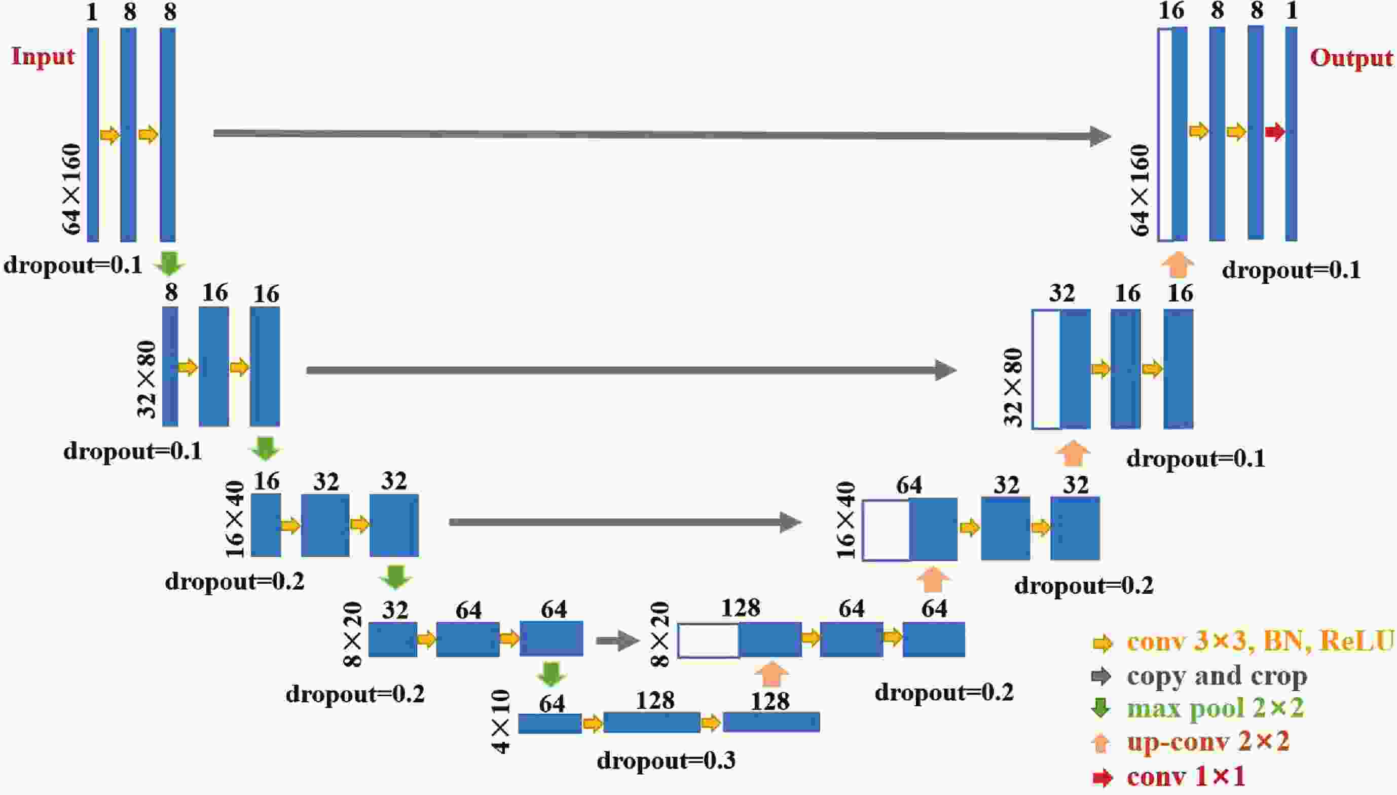

Figure 1.  The U-Net architecture used to represent the relationship between zonal (and meridional) wind stress anomalies and SSTAs in the tropical Pacific. Each blue box represents a multi-channel feature map, and the white boxes represent copied feature maps. The size of the feature map is denoted on the left of the box.

Taking the U-Net architecture for output zonal wind stress anomalies as an example (Fig. 1): an input SSTA for the tropical Pacific (31.5°S−31.5°N, 123.5°E−77.5°W) is first linearly interpolated onto a 64 × 160 uniform grid in the encoder path (left side). To connect with the correspondingly cropped feature maps from decoder paths, two convolution modules (yellow arrows) and a 2 × 2 max pool layer (green arrows) are applied to multiply the number of feature maps (blue boxes) and halve the image size. Each convolution module includes a 3 × 3 convolutional layer, a batch normalization layer, and a ReLU activation function. The number of channels (the number above the blue boxes) in the convolution layer multiplies, and directly determines the number of feature maps. In particular, each module has a dropout function of different sizes to randomly eliminate neurons. To prevent overfitting, the more feature maps taken in a module, the larger the dropout rate (the number below the blue boxes). After performing the encoder path four times, the number of feature maps changes to 64 and the image size is transformed to 4 × 10. In the last encoder path, two convolution modules are used to double the number of feature maps to 128. Subsequently, the feature maps are upsampled (orange arrows) and connected (gray arrows) to the previous encoder output (white boxes). The decoder paths (right side) also adopt two convolution modules (yellow arrows) with dropout functions, reducing the number of feature maps by half. After four iterations, a 1 × 1 convolution layer (red arrows) is selected as the last layer to yield an output zonal or meridional wind stress anomaly field with the same grid as the input.

Here, the U-Net models were built by the TensorFlow library (Abadi et al., 2016) and trained with the Adam optimizer (Kingma and Ba, 2015). The learning rate was assigned to be 1 × 10⁻³ for training 100 epochs and reduced to 1 × 10⁻⁵ for fine-tuning 30 epochs. In addition, the mean square error (MSE) was adopted as a loss function. After training and fine-tuning, the U-Net models yielded two versions of model parameters that can represent nonlinear relationships (${f_{{\text{ua}}}}$ and ${f_{{\text{va}}}}$) between SSTAs (${\text{Ta}}$) and zonal wind stress anomalies (${\text{Ua}}$) or meridional wind stress anomalies (${\text{Va}}$) in the ocean–atmosphere coupled models. These are symbolically written as follows:

Monthly U-Net models were also trained with the TensorFlow library and Adam optimizer. After training 50 epochs with a 1 × 10⁻³ learning rate and fine-tuning 20 epochs with a 1 × 10⁻⁵ learning rate, the monthly U-Net models obtained 2 × 12 versions of model parameters for calculating zonal and meridional wind stress anomalies in all months. The relationship for each month ($m$, $m = $1, …, 12) is symbolically written as:

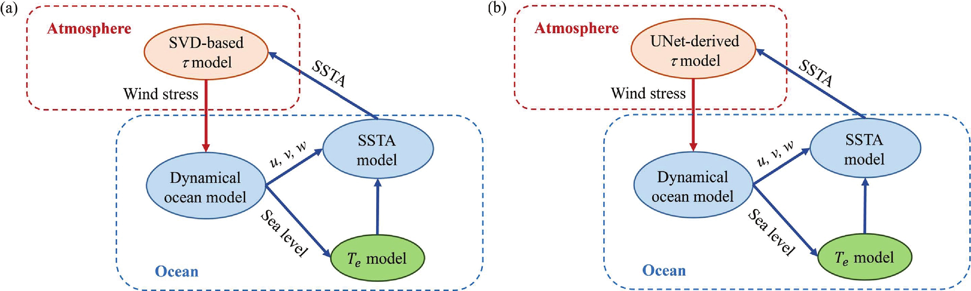
As an improved intermediate coupled model, the IOCAS ICM is comprised of an intermediate ocean model and an SVD-based $\tau $ model (Fig. 2a). The dynamical ocean component of the original IOCAS ICM is an intermediate-complexity model developed by Keenlyside and Kleeman (2002), divided into a linear and a nonlinear component. This model represents the evolution of dynamical ocean variables in the tropical Pacific, including sea level (SL), sea pressure, the horizontal currents in the surface mixed layer, and the vertical velocity at the mixed layer bottom. The SSTA model is inserted into the dynamical ocean model to depict the evolution of interannual SST variability in the surface mixed layer. Previous studies have shown that interannual SL variability is closely related to ${T_e}$ in the tropical Pacific (Zhang et al., 2004). A distinctive feature of the ICM includes a non-local empirical parameterization for ${T_e}$ to optimize the SST simulations. In its original version, the ICM had an SVD-based statistical atmospheric module for calculating the interannual wind response. The SVD-based $\tau $ model is constructed with historical data from 1963 to 1996. For more details, the SVD analysis process retains the first five dominant modes and considers seasonal variation. More detailed descriptions of the ICM are provided by Zhang and Gao (2016a, b).

Figure 2.  Schematic diagrams showing the structures of (a) the ICM and (b) the ICM-UNet. The ICM is comprised of an SVD-based wind stress ($\tau $) model and an intermediate ocean model (IOM) consisting of a dynamical ocean model, an SSTA model, and an empirical anomaly model for $ {T}_{e} $. In the ICM-UNet, the SVD-based $\tau $ model is replaced by the UNet-derived $\tau $ model, and the ocean component is the same as that of the original IOCAS ICM.

The ICM constructed in this study (ICM-UNet) replaces the SVD-based $\tau $ model in the atmospheric module with the UNet-derived $\tau $ model (Fig. 2b). Thus, the ICM-UNet mainly contains a dynamical ocean model, an SSTA model nested in the dynamical ocean model, an empirical anomaly model for the temperature of subsurface water entrained into the surface mixed layer (${T_e}$), and the ${\tau _{{\text{UNet}}}}$ model. The structure of ICM-UNet remains the same whether or not it considers the seasonality of wind stress anomalies.

Experiments show that the ${\tau _{{\text{UNet}}}}$ model trained with CMIP6 products can well represent the relationship between SSTAs and interannual wind stress anomalies in the ICM (details in section 3.1). In this study, the ${\tau _{{\text{UNet}}}}$ model entirely replaces the SVD-based $\tau $ model used in the atmospheric module for obtaining the zonal and meridional wind stress anomalies desired in the coupling procedure. The ${\tau _{{\text{UNet - ann}}}}$model is constructed using all data without distinguishing months. Considering seasonal variations, this study also constructed a seasonally varying model, the ${\tau _{{\text{UNet - mon}}}}$ model. These two ${\tau _{{\text{UNet}}}}$-integrated ICMs are denoted as the ICM-UNet$_{{\text{ann}}}$ and ICM-UNet$_{{\text{mon}}}$, respectively.

During the integration process, the original ICM dynamical ocean part operates through Fortran programs, while the atmospheric ${\tau _{{\text{UNet}}}}$ model is built using Python programs. Since dynamical oceanic models and AI-based atmospheric models adopt two kinds of computer languages, the text-file interaction is chosen here to integrate different modeling parts. Through Fortran programs, the dynamical ocean model generates the ocean anomaly fields, including currents and SL anomalies. Next, the SL anomalies are used to calculate ${T_e}$ anomalies in the ${T_e}$ model, followed by obtaining SSTAs based on the SST anomaly equation. In due course, SSTAs are then saved in offline text files following a uniform format and input into the Python programs used to build the ${\tau _{{\text{UNet}}}}$ model. The corresponding wind stress anomalies are output through these Python programs. The obtained zonal and meridional wind stress anomalies are also saved in offline text files following the same format so that dynamical oceanic models can obtain them afterward. Finally, the wind stress anomalies are extracted with Fortran programs and applied to force the dynamical ocean model, thus completing the whole coupling process. Throughout the coupling process, the atmospheric and oceanic component models exchange anomaly information once a day.

The modeled region covers the tropical Pacific and Atlantic oceans (31°S−31°N, 124°−30°E), however, only the Pacific part (31°S−31°N, 124°E−78°W) is considered here. The realistic distribution of sea and land is adopted in the horizontal direction, and the vertical direction assumes a flat-bottomed ocean with a depth of 5500 m. The model has a zonal resolution of 2°. The meridional resolution is 0.5° within 10°S−10°N and decreases to 3° towards its northern and southern boundaries. So, it is necessary to interpolate anomalies before and after using the ${\tau _{{\text{UNet}}}}$ model to accommodate different horizontal grids.

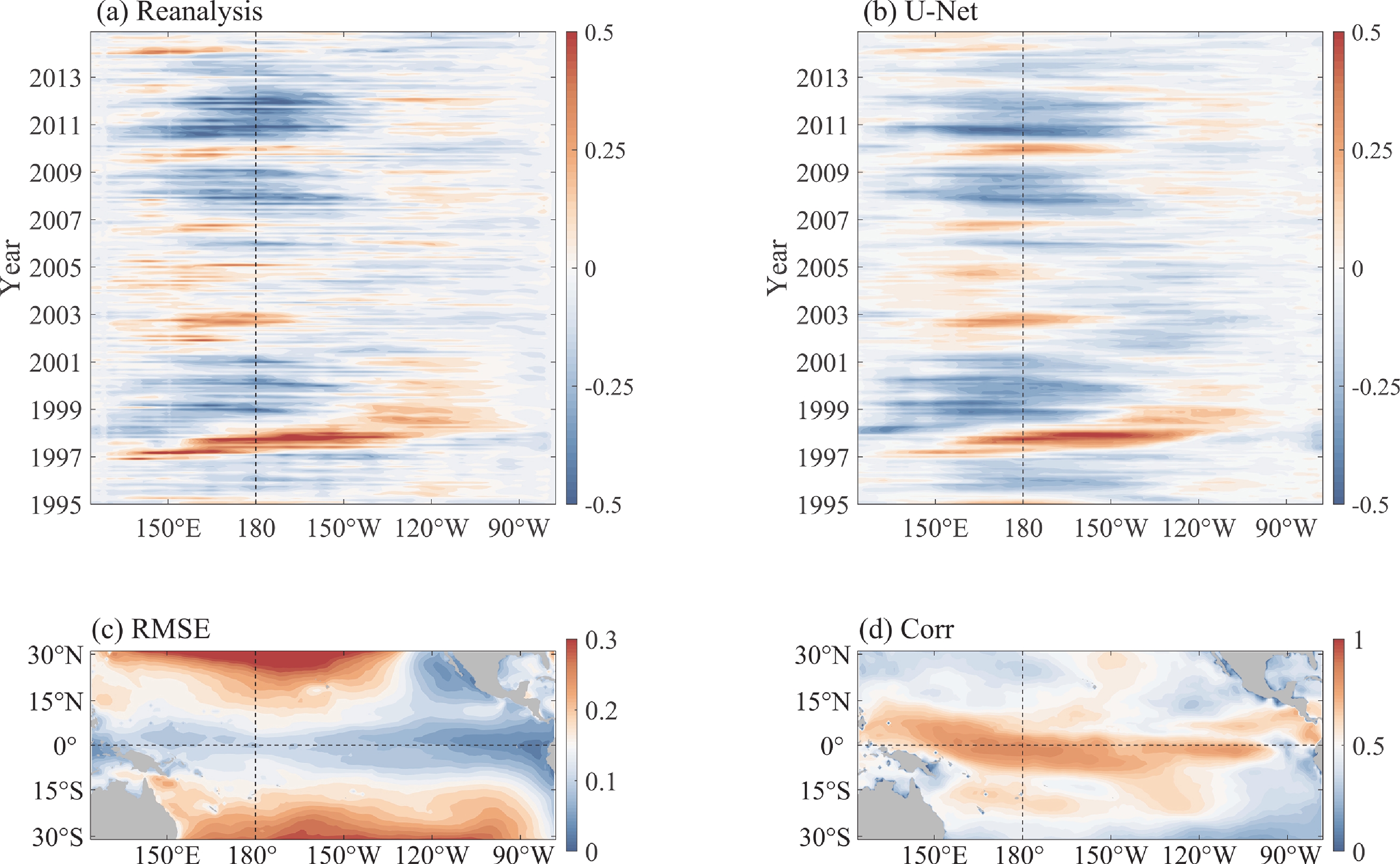
This section mainly assesses the test results of the U-Net models. The zonal wind stress anomaly field along the equator obtained from reanalysis data is shown in Fig. 3a, which reflects the actual evolution of the zonal wind field from 1995 to 2014. For example, during El Niño events (e.g., 1997–98), a strong westerly wind anomaly first erupted over the central-western Pacific and gradually moved eastward and weakened; during La Niña events (e.g., 2011–12), the central equatorial Pacific Ocean exhibits continuous easterly wind anomalies. As shown in Fig. 3b, the estimations derived from the U-Net model essentially capture the same spatiotemporal patterns as in Fig. 3a, indicating that the U-Net model can represent the nonlinear relationship between SSTAs and interannual wind stress anomalies. Consistent with the quasi-periodic variability of ENSO events, westerly and easterly wind anomalies occur alternately over the central basin.

Figure 3.  Zonal wind stress anomaly fields (units: dyn cm⁻²) along the equator during the period 1995−2014: (a) reanalysis data and (b) estimated from the U-Net model; (c) the RMSE; (d) Corr between the estimated zonal wind stress anomalies and reanalysis data. SSTAs are used as input data for the U-Net model.

During model testing, the root-mean-square error (RMSE) and correlation coefficient (Corr) between simulations and reanalysis data are chosen to evaluate the performance of the U-Net models quantitatively. Specifically, the RMSE measures the differences between the simulated and reanalysis wind stress anomalies, and the Corr measures the linear correlation. The RMSE and Corr are defined as follows:

Here, N is the number of months during the test period (1995−2014; taken as N=240); ${X_j}$ and ${Y_j}$ denote the reanalysis and simulated wind stress anomalies; ${\overline X_j}$ and ${\overline Y_j}$ are their averaged values in the j-th month.

Figures 3c and 3d show that the regions near the equator possess low RMSE and high Corr. In particular, the RMSE is lower near the eastern equatorial Pacific, mostly under 0.15 and the Corr is higher in the western Pacific, generally over 0.5. This is mainly because the horizontal distributions of RMSE and Corr are related to the spatial characteristics of variables, with low errors and high correlations in regions where SSTAs and wind stress anomalies covary coherently. However, there are still large discrepancies in the off-equatorial and land-edge areas.

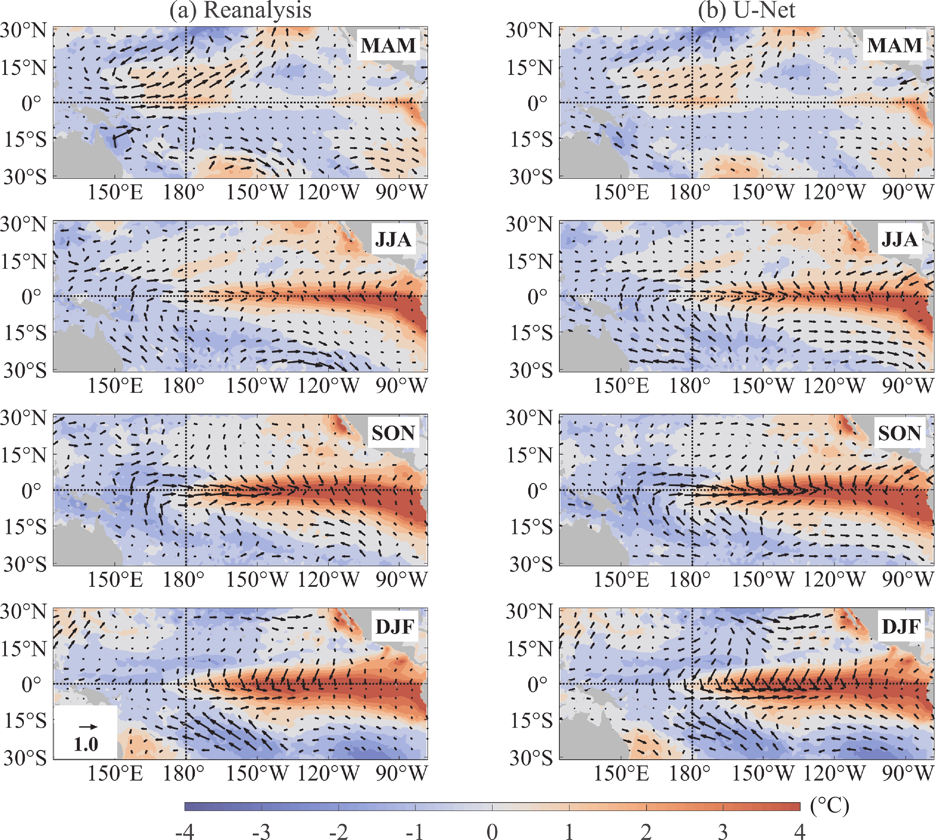
To evaluate the simulation capability of the U-Net models in detail, Fig. 4 displays the horizontal distribution of SSTAs (contours) and wind stress anomalies (vectors) during the El Niño development phase. This figure explicitly indicates the spatiotemporal evolution of interannual wind stress anomalies from different phases during El Niño events. The interannual wind response to SSTA calculated by the U-Net models is generally consistent with reanalysis data, proving that the simulations are reliable. For instance, a warm SST anomaly originating near the date line is accompanied by a westerly wind anomaly over the western Pacific. As the El Niño event intensifies, this warm anomaly gradually spreads to the east, while the westerly anomaly and cross-equatorial trade winds appear in the central basin. The results obtained from the monthly U-Net models have no significant difference, which is not described here (but can be seen in Figs. S3 and S4 in the ESM).

Figure 4.  Horizontal distribution of SSTAs (contours; units: °C) and wind stress anomalies (vectors; units: dyn cm⁻²) during the development phase of an El Niño event (from March 1997 to February 1998). SSTAs are derived from reanalysis data; wind stress anomalies are derived from (a) reanalysis data and (b) the U-Net models, respectively. The scale for wind stress vectors, given by the black arrow in the lower left corner, indicates 1.0 dyn cm⁻². The figures show the mean values for every three months, and the corresponding months are displayed in the upper right corner of each figure for convenience.

In summary, the test results of the U-Net models from 1995 to 2014 can effectively depict the temporal evolution and spatial distribution of interannual wind stress anomalies in the tropical Pacific, indicating that the ${\tau _{{\text{UNet}}}}$ model is a credible tool to represent the nonlinear relationship between SSTAs and wind stress anomalies.

This section analyzes the simulations of ENSO using the ICMs from multiple perspectives. The evolutions of SST, zonal wind stress, and SL anomalies along the equator in the ICM-UNet$_{{\text{ann}}}$ and ICM-UNet$_{{\text{mon}}}$ are shown in Fig. 5. These figures present coherent interannual oscillations in the atmospheric and oceanic anomaly fields, demonstrating the feasibility of integrating AI-derived models with physical models. For example, as shown in Figs. 5a and b, the SSTAs are continuous, with the maximum anomalies being concentrated in the central-eastern equatorial Pacific and the maximum wind stress anomalies being located near the date line (Figs. 5c, d). Consistent with that found in nature, one typical feature of zonal wind stress anomalies includes its eastward propagation from the western equatorial Pacific during the development of ENSO events. Besides, the SL anomalies display a distinct phase propagation feature along the equator: initially occurring in the western Pacific and then spreading eastward as they amplify (Figs. 5e, f). The simulation results in the ICM-UNet$_{{\text{ann}}}$ and the ICM-UNet$_{{\text{mon}}}$ have similar spatiotemporal characteristics, except that the amplitude of the El Niño event slightly decreases and the amplitude of the La Niña event slightly increases when using the ${\tau _{{\text{UNet - mon}}}}$ model.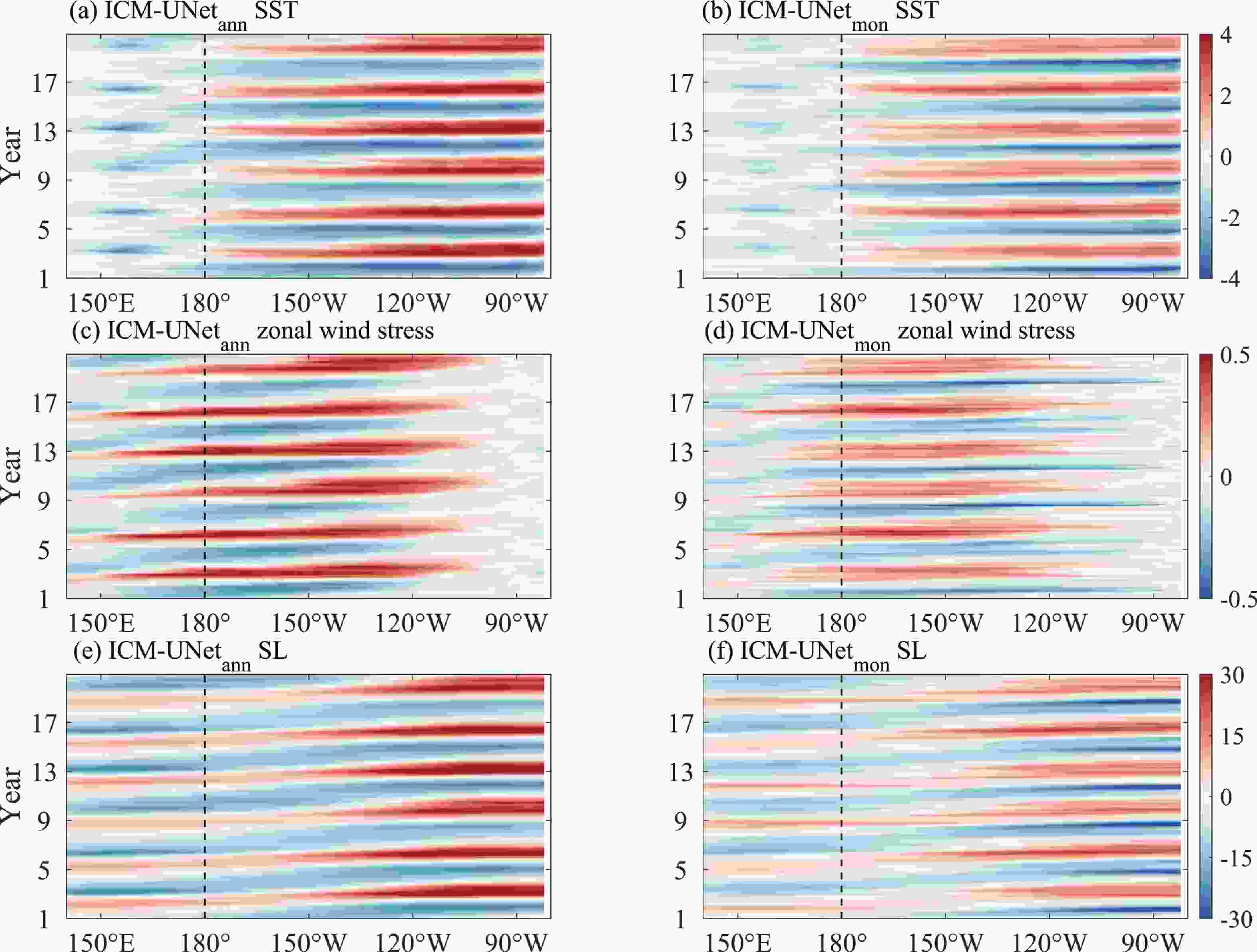

Figure 5.  Evolution of SST (top panels; units: °C), the zonal wind stress (middle panels; units: dyn cm⁻²), and SL (bottom panels; units: cm) anomalies along the equator for (a, c, e) ICM-UNet$_{{\text{ann}}}$ and (b, d, f) ICM-UNet$_{{\text{mon}}}$.

Measuring the averaged SSTAs in different key regions of the tropical Pacific is insightful for analyzing the ENSO events (Trenberth and Stepaniak, 2001). Thus, we also calculated the time series of SSTAs in the Niño-3.4 region (5°N−5°S, 170°−120°W), Niño-4 region (5°N−5°S, 160°E−150°W), Niño-3 region (5°N−5°S, 150°−90°W) and Niño-1+2 region (0−10°S, 90°−80°W), respectively (Fig. 6). The results illustrate that the ICM-UNet is reliable when simulating interannual SSTA variability in the tropical Pacific. Compared with simulations of the original IOCAS ICM, the results obtained from the ICM-UNet have a more definite 3.5-year cycle, and the regions with stronger amplitudes appear in the eastern Pacific. In the Niño-3.4 region, the amplitude degrades with simulations from the ICM-UNet (Fig. 6a). As shown in Figs. 6b and c, the SSTAs simulated by the ICM-UNet have robust variations in the eastern Pacific and only slight variations in the central Pacific. In the Niño-1+2 region, the simulated amplitudes are similar for all models, while the durations become shorter when using the ${\tau _{{\text{UNet}}}}$ model (Fig. 6d). Additionally, the simulated amplitudes from the ICM-UNet$_{{\text{mon}}}$ are slightly weaker than those from the ICM- UNet$_{{\text{ann}}}$, but the difference is not substantial.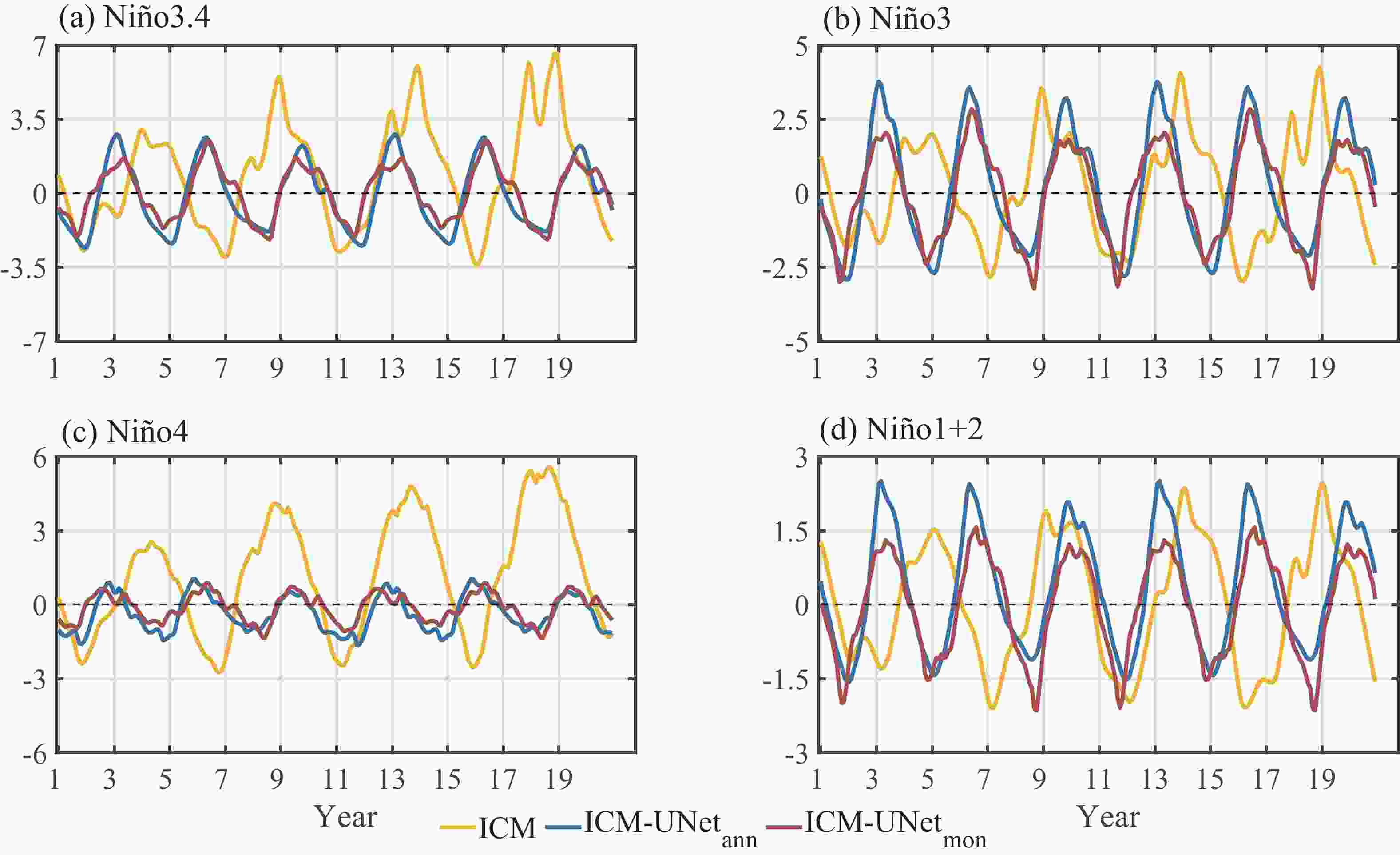

Figure 6.  Time series of SSTAs (units: °C) averaged over (a) the Niño-3.4 region, (b) the Niño-3 region, (c) the Niño-4 region, and (d) the Niño-1+2 region, respectively.

To quantify the spatial structure of SST interannual variability, Figs. 7a−d show the spatial distributions of its standard deviation in the tropical Pacific. From the reanalysis data, the magnitude of standard deviation is relatively small, with the strongest interannual variability being located in the eastern equatorial Pacific and near the Peruvian coast. In the simulations using the original ICM, significant SST variability tends to occur in the central Pacific and extends eastward (Fig. 7b). In contrast, the ICM-UNet can better simulate the maximum variance center in the eastern Pacific but still overestimates the amplitude (Figs. 7c, d). It is worth noting that the results obtained from the ICM-UNet$_{{\text{mon}}}$ display a slight weakening of the variability. Therefore, the ICM-UNet$_{{\text{mon}}}$ can simulate the structure and amplitude of SST interannual variability in the eastern equatorial Pacific more accurately.

Figure 7.  (a)–(d) Spatial distributions of the standard deviation for SSTAs (units: °C); (e) seasonal variations in the standard deviation of Niño-3.4 SSTA (units: °C) as a function of calendar months; (f) power spectra of the Niño-3.4 SSTA. SSTAs are derived from (a) reanalysis data, (b) ICM, (c) ICM-UNet$_{{\text{ann}}}$, and (d) ICM-UNet$_{{\text{mon}}}$, respectively. The simulations are based on the model years 1−20, and the reanalysis data are calculated during the period 1967−78, respectively.

Previous studies have shown that ENSO events tend to lock their peaks into boreal winters (Tziperman et al., 1998). In all simulations, the standard deviation of the Niño-3.4 SSTA is at minimum in late spring and maximum in winter, indicating that the ENSO phase-locking features are well captured in the ICM-UNet (Fig. 7e). However, the amplitude of the standard deviation is too large when simulated by the original ICM. In contrast, the simulations are more reasonable when using the ICM-UNet$_{{\text{ann}}}$. In addition, the magnitude of the standard deviation drops again when using the ICM-UNet$_{{\text{mon}}}$, but the months when the maximum and minimum occur are slightly delayed compared to the reanalysis results.

Figure 7f presents the power spectrum of the Niño-3.4 SSTA. In the reanalysis results, the main period of the Niño-3.4 SSTA is 3−4 years and the broad spectrum is between 2−5 years, which is generally consistent with nature. In comparison, the original ICM simulations exhibit too much power with wide bandwidth, indicating a peak occurring at 4−6 years. This discrepancy in the simulated ENSO periodicity has been noticeably alleviated when using the ICM-UNet. The ICM-UNet simulations display power spectra with lower peaks and narrower bandwidths. The power in the ICM-UNet$_{{\text{mon}}}$ simulations is weaker than that of the ICM-UNet$_{{\text{ann}}}$ but is still overestimated. Overall, the results derived from the ICM-UNet are more reasonable concerning the principal periods and spectral ranges.

To summarize, the ICM-UNet can simulate the evolutions of the oceanic and atmospheric anomaly fields in the equatorial Pacific. When using the ${\tau _{{\text{UNet}}}}$ model to replace the SVD-based $\tau $ model in the atmospheric module, the simulated SSTAs exhibit spatiotemporal variability characteristics, with the maximum centers being located in the eastern equatorial Pacific. The simulation results slightly improve when using the ICM-UNet$_{{\text{mon}}}$, but the changes are not significant. These physically reasonable results demonstrate the feasibility of combining AI-based wind models with ocean–atmosphere coupled models.

This section presents an ocean-only case study for the 1997−98 El Niño event. Here, wind stress anomalies obtained from the ${\tau _{{\text{UNet - ann}}}}$ model, the ${\tau _{{\text{UNet - mon}}}}$ model, and the SVD analysis are used to force the same ocean component of the ICM, respectively. The ocean component of the ICM mainly consists of an intermediate ocean model (IOM), so these models are denoted as IOM-UNet$_{{\text{ann}}}$, IOM-UNet$_{{\text{mon}}}$, and IOM-SVD, respectively. The SVD analysis mentioned here is built in the same way as mentioned in section 2.3. As shown in Figs. 8a−d, all the simulations can represent the evolution of SSTAs in the equatorial Pacific. The general performance of the IOM-SVD is marginally better than the IOM-UNet$_{{\text{ann}}}$ and IOM-UNet$_{{\text{mon}}}$, but there are spatial deviations when simulating typical ENSO events.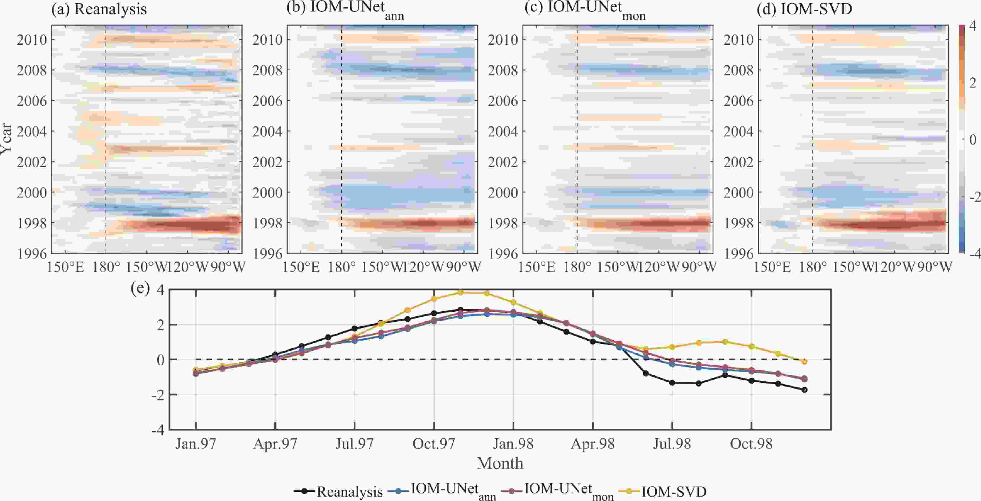

Figure 8.  (a)–(d) SSTAs (units: °C) along the equator during the period 1996−2010; (e) time series of SSTAs (units: °C) averaged over the Niño-3.4 region from January 1997 to December 1998. SSTAs are derived from (a) reanalysis data, (b) IOM-UNet$_{{\text{ann}}}$, (c) IOM-UNet$_{{\text{mon}}}$, and (d) IOM-SVD, respectively.

Taking the simulations of the 1997−98 El Niño event as an example: compared with the IOM-SVD, both the IOM-UNet$_{{\text{ann}}}$ and the IOM-UNet$_{{\text{mon}}}$ can simulate the amplitudes and phases of the SSTAs in the Niño-3.4 region more precisely (Fig. 8e). The amplitude of the SSTAs simulated by the IOM-UNet$_{{\text{mon}}}$ is much closer to the reanalysis data throughout the El Niño cycle. During the peak of the El Niño event, the difference between the IOM-UNet$_{{\text{mon}}}$ simulation and reanalysis data is less than 0.5°C; the SSTAs simulated by the IOM-SVD are much larger, with a maximum difference of approximately 1°C. However, the amplitudes of SSTAs are underestimated in all models during the development period. Moreover, it is well known from the reanalysis data that the warm-cold phase transition of this El Niño event occurred in May and June 1998. The phase transition period of the IOM-UNet simulations is June and July, close to the reanalysis data; but the simulated SSTAs of the IOM-SVD rise again in July, and the phase transition is postponed until November and December.

The horizontal distribution of the SSTAs from July 1997 to April 1998 (Fig. 9) clarifies these results from other perspectives. The simulations show that the warm SSTAs in the eastern equatorial Pacific continuously expanded from July 1997 to January 1998. Then, they gradually weakened in the following months, similar to the reanalysis data. In particular, the maximum SSTAs simulated by the IOM-UNet are concentrated in the eastern equatorial Pacific and along the Peruvian coast (120°−80°W), which is close to the actual situation. In contrast, the maximum center of the SSTAs simulated by the IOM-SVD is slightly westward (150°−120°W).

Figure 9.  Horizontal distributions of SSTAs (units: °C) during an El Niño event (from July 1997 to April 1998). SSTAs are derived from (a) reanalysis data, (b) IOM-UNet$_{{\text{ann}}}$, (c) IOM-UNet$_{{\text{mon}}}$, and (d) IOM-SVD, respectively. The corresponding months are displayed in the upper-right corner of each figure for convenience.

For a comprehensive comparison, the RMSEs of the SSTA simulations in the tropical Pacific during 1996−2010 are intuitively displayed in Figs. 10a−c, and the differences in RMSE are shown in Figs. 10d and e. In all simulations, the regions with higher RMSEs are concentrated near the equator and at the edges of the zone. The RMSEs in the IOM-UNet simulation are generally smaller than those in the IOM-SVD case, especially in the central equatorial Pacific. However, the IOM-UNet models have bigger RMSEs than the IOM-SVD model in the eastern Pacific, which is due to the U-Net models overfitting the nonlinear signals in this region. In comparison, the simulation from the IOM-UNet$_{{\text{mon}}}$ is more accurate, with its RMSE being smaller than that from the IOM-SVD in more than 80% of areas.

Figure 10.  The RMSEs between the simulated SSTAs and reanalysis data from 1996 to 2010. The simulated SSTAs are derived from (a) IOM-UNet$_{{\text{ann}}}$, (b) IOM-UNet$_{{\text{mon}}}$, and (c) IOM-SVD, respectively; the differences in RMSE are shown in (d) and (e).

To summarize, the ocean component of the ICM forced by different wind stress anomaly fields can simulate the spatiotemporal evolution of the 1997−98 El Niño event. In contrast, the simulations present more feasible phases and amplitudes when using the wind stress anomalies derived from the ${\tau _{{\text{UNet}}}}$ model as the forcing fields for ocean-only experiments. The results are slightly better when using the ${\tau _{{\text{UNet - mon}}}}$ model output as forcing fields, but the difference is minor. The comparisons further demonstrate that forcing the ocean component with the ${\tau _{{\text{UNet}}}}$-derived wind stress anomaly fields can provide proper simulations of typical El Niño events and reduce simulation discrepancies in the central Pacific.

As the strongest interannual climate signal, ENSO plays a fundamental role in the coupled ocean–atmosphere system over the tropical Pacific (Cai et al., 2021). In traditional studies in physical oceanography, dynamical and statistical models are generally used to simulate and predict ENSO events, including the ICMs. For simulations of ENSO events, the precise representations that establish the relationship between SST and wind stress variabilities are essential. However, statistical methods, such as EOF and SVD analysis, only provide linear responses of wind stress anomalies to SSTAs. However, in the recent decade, DL techniques have been extensively applied in climate studies (Taylor and Feng, 2022). As a prospective technique for climate modeling, DL can overcome the weaknesses of statistical methods by scaling down the manual pre-processing and subsequent processing, giving more space for the automatic tuning of neural networks. Previous studies have shown that AI-based models can represent the nonlinear relationships between different variables after training with extensive data, and their direct integrations with physics-based dynamical models are active areas of research (Irrgang et al., 2021).

In this study, the U-Net models were constructed to represent the nonlinear relationship between SSTAs and interannual wind stress anomalies, and the ${\tau _{{\text{UNet}}}}$ model was used to replace the SVD-based $\tau $ model for integration with the IOCAS ICM. Due to the seasonal dependence of interannual wind stress anomalies on SSTAs, this study also constructed the ${\tau _{{\text{UNet - mon}}}}$ model. The simulations in the ICM-UNet can depict the quasi-periodic variation of atmospheric and oceanic anomaly fields in the equatorial Pacific. In particular, the spatiotemporal evolution of SSTAs is consistent with the physical patterns. These results suggest that AI-derived models can be adopted as components in the dynamical models that represent ENSO events. In addition, the ocean component of the IOCAS ICM forced by the ${\tau _{{\text{UNet}}}}$-derived wind stress anomalies can reasonably characterize typical El Niño events. This case study reconfirms the feasibility of integrating AI-based wind models with dynamical ocean models, providing a promising method for the integration of AI-based models with physics-based models.

However, this study has only analyzed the initial integrations of the ${\tau _{{\text{UNet}}}}$ model with the oceanic component of the ICM, and many issues remain. For example, the evolution of variables such as SSTAs is quite regular in the simulation results, which fails to reflect the diversity of ENSO events. Because neural networks are data-driven, the nonlinear relationships between variables can be established and comprehended without physical assumptions. The original ICM represents the linear relationship between SSTAs and wind stress anomalies based on SVD analysis. As a coupled model, changing any components in the ICM would induce unexpected effects. For example, the integration of the ${\tau _{{\text{UNet}}}}$ model may weaken the variability strength of other variables in the central Pacific. Since the integration of AI-based models with physics-based models is a preliminary attempt, this study ignored the influence of incorporating the ${\tau _{{\text{UNet}}}}$ model on the other components. This approach for integrating AI-derived models with dynamical models requires additional validations to ensure the model still follows the fundamental physical laws. In addition, the integration model calculates slowly and consumes numerous computing resources. Due to the ICM exchanging variable information once a day, transferring anomalies with text files significantly prolongs the running time. Meanwhile, extensive text files take up computational space and constantly exhaust computing resources. It takes 25 minutes to obtain the simulations of one model year.

Thus, there are still several tasks to accomplish in the future. First, the ${\tau _{{\text{UNet}}}}$ model should be adjusted to enhance their adaptability for ocean–atmosphere coupled models. The ICM-UNet only still obtains regular interannual variability of oceanic and atmospheric anomalies, which cannot capture the diversity of ENSO events. It is possible to make the simulation results closer to reality by optimizing the parameters of the ${\tau _{{\text{UNet}}}}$ model or constructing more advanced AI-based models. Secondly, various validations are required to illustrate the effects of integrating the ${\tau _{{\text{UNet}}}}$ model on the other components of the ICM. If necessary, it is permissible to adjust these modules to guarantee that the ICM-UNet follows the basic ocean–atmosphere dynamical processes. Third, we need to speed up the file interaction and improve the utilization of computational resources. By speeding up the file interaction, long-term simulations with shorter computational times are realizable, considerably increasing the usefulness of the coupled model. Finally, future studies can construct different AI-based models to represent the nonlinear relationships between vital physical variables and integrate them with other ocean-atmosphere coupled models through the method demonstrated in this study. This approach is promising for becoming a useful integration technique of AI-based models and dynamical models in physical oceanography and meteorology.

Acknowledgements. The authors wish to thank the two anonymous reviewers for their comments that helped to improve the original manuscript. This research was supported by the National Natural Science Foundation of China (NFSC; Grant No. 42030410), Laoshan Laboratory (No. LSKJ202202402), the Strategic Priority Research Program of the Chinese Academy of Sciences (Grant No. XDB40000000), and the Startup Foundation for Introducing Talent of NUIST.

Electronic supplementary material: Supplementary material is available in the online version of this article at https://doi.org/10.1007/s00376-023-3179-2.