


 DownLoad:


-
The way in which the notion of probability is embedded into weather forecasting differs from all other forecasting domains. Numerical weather prediction (NWP) ensemble forecasts are derived by perturbing the analysis and evolving each perturbed set of initial conditions forward in time according to the governing laws of dynamics and physics (Bauer et al., 2015). Even though ensemble weather forecasting has matured over the past half-century or so, the produced forecasts are still often under-dispersed (Vannitsem et al., 2018; Lauret et al., 2019), resulting in an underestimation of the uncertainty (Fortin et al., 2006). Consequently, various ways of calibrating those under-dispersed forecasts find their relevance. Statistically, although other context-dependent definitions exist (e.g., Mayer and Yang, 2023a), calibration (also known as reliability) mostly refers to the consistency between the distributional forecasts and the corresponding observations. Informally, calibration means that the nominal coverage rate of prediction intervals (PIs) is equal to the empirical one, e.g., PIs of 80% coverage rate should cover 80% of the observations (Lauret et al., 2019). According to the typology of Yang and van der Meer (2021), who conducted a detailed review of post-processing techniques, calibration is a type of probabilistic-to-probabilistic (P2P) post-processing technique that can improve the reliability of uncalibrated raw ensembles via (1) distributional regression methods such as ensemble model output statistics (EMOS), (2) methods of dressing, and (3) quantile regressions (QRs). These three (classes of) methods are briefly reviewed in the following three paragraphs. Another detailed overview of post-processing methods and recent developments was conducted by Vannitsem et al. (2021).
EMOS is a classic P2P post-processing method first proposed by Gneiting et al. (2005). It assumes that the predictive distribution of the response variable is normal, which can be written as
where
$ {Y}_{t} $ is the response variable,$ \{{x}_{t,1},{x}_{t,2}, \dots ,{x}_{t,p}\} $ are ensemble members at time$ t $ , with variance$ {s}_{t}^{2} $ , and$ \{{m}_{0}, 1, \dots , {m}_{p},{n}_{0},{n}_{1}\} $ are EMOS model parameters, which can be estimated by maximizing the likelihood or minimizing the continuous ranked probability score (CRPS). Moving beyond its basic form, one should note that the Gaussian predictive distribution can be replaced by other parametric distributions, although such extensions should not concern the present work. Regardless, EMOS, and more generally, distributional regression, produce parametric predictive distributions, of which the predictive performance depends heavily upon the validity of the distributional assumption made.The core idea of the methods of dressing is to modify each member of a dynamical ensemble forecast with some past errors to improve reliability. Roulston and Smith (2003) proposed a method called “best-member dressing,” in which each ensemble member is dressed with errors resampled from the past “best-member” errors. Wang and Bishop (2005) found that results of the best-member dressing still lack reliability, and proposed a 2nd-moment-constrained dressing method. In another attempt, Fortin et al. (2006) sorted the members of each ensemble, and then calculated the best-member errors for the ensembles whose best members are the
$ k $ th ensemble member. Finally, Bayesian model averaging (BMA) can also be considered as a form of dressing. It dresses a distribution or a probability density distribution (PDF) onto each ensemble member, and then linearly combines all dressed PDFs to obtain the final predictive distribution (Raftery et al., 2005), which is given bywhere
$ {f}_{t,i}\left(z|{z}_{t,i}\right) $ is the dressed PDF for the$ i $ th member,$ {g}_{t}\left(z\right) $ is the PDF of the combined forecast,$ {w}_{i} $ is the combination weight, and$ z $ is a generic variable representing the argument of density functions. The predictive distributions resulting from BMA are semiparametric in nature, and are therefore slightly more flexible than EMOS-based parametric predictive distributions.In practice, it is difficult, or not possible, to conclude with absolute certainty whether a variable of interest strictly follows a certain (semi) parametric distribution. In this regard, QR as proposed by Koenker and Bassett (1978), which requires no distributional assumption, is often preferred and can usually achieve better calibration performance than the other two classes of P2P post-processing methods (Bremnes, 2004; Yagli et al., 2020). Differing from regular regression problems, in which the conditional mean is estimated, the target variable of QR is the conditional quantile. In terms of parameter estimation, instead of minimizing the sum of square errors, QR minimizes the sum of pinball losses, which depends on some quantile level
$ \tau \in \left[\mathrm{0,1}\right] $ . Since QR is a regression, it has many statistical and machine-learning variants. In the case of the former, one possible way is to introduce regularization into QR, which gives rise to penalized QR. In the case of the latter, the extensions are typified by quantile regression neural network (QRNN; Cannon, 2011) and quantile regression forest (QRF; Meinshausen, 2006; Taillardat et al., 2016).A long-standing problem of QR-based methods, nevertheless, is quantile crossing, which greatly limits the interpretability of the regression results. More specifically, given two quantile levels
$ {\tau }_{1} $ and$ {\tau }_{2} $ ,$ {\tau }_{1} < {\tau }_{2} $ , quantile crossing occurs if$q_{\tau 1} > q_{\tau 2} $ (Moon et al., 2021). This problem violates the basic principle that the cumulative distribution function (CDF) should be monotonically increasing (Moon et al., 2021). Chernozhukov et al. (2010) bypassed this problem by simply reordering those nonmonotone quantile forecasts. Although the reordered estimates are found to be close to the true quantiles, it does not extend to extreme cases as to cover heavy tails beyond the sample (Kithinji et al., 2021). Evidently, a method that can directly produce ordered quantiles without reordering would be much more reliable and thus desirable. So far, numerous non-crossing QR methods have been proposed. For instance, Liu and Wu (2009) estimated quantile functions in a stepwise fashion. When estimating the quantile function of the next quantile level, inequality constraints are imposed on the regression coefficients to ensure that the estimated quantile equations do not cross with the current one. Bondell et al. (2010) generated non-crossing quantiles of endpoints of a convex hull by imposing constraints on the regression coefficients of linear quantile regression (LQR), and assumed that the quantiles of the points inside convex hull were linear combinations of those of endpoints. In El Adlouni and Baldé (2019), Bayesian non-crossing QR was introduced for heavy-tailed distributions based on extreme index estimation. However, most non-crossing methods are only applicable to LQR and are not valid for complex machine-learning regression models such as QRNN, which therefore greatly confines their generalization and uptake.The first non-crossing remedy for QRNNs was proposed by Cannon (2018), which constrained the parameters of all hidden and output layers to be positive and used monotone activation functions to avoid the crossing problem. However, since all the layers were imposed with restrictions, this approach is not applicable to other models, except feedforward neural networks. Moon et al. (2021) developed another strategy preventing quantile crossing by imposing inequality constraints on the weights of the output layer. The proposed non-crossing strategy is more flexible, but the trained model still requires post-correction. Whilst modifying the network setting is one approach, one can also address quantile crossing by working with the predictive distribution itself. For instance, both Gasthaus et al. (2019) and Bremnes (2019) used splines to approximate a monotonically increasing CDF, in which error may be introduced in conversion from the CDF to quantiles, and performance depends on the number of knots. In Bremnes (2020), Bernstein basis polynomials were employed to approximate an increasing CDF, but this approach is still confronted by those issues that confronted Gasthaus et al. (2019) and Bremnes (2019).
After reviewing the existing literature, a couple of facts can be consolidated. First, modern ensemble weather forecasts from NWP are often under-dispersed, which necessitates post-processing in the style of calibration. Second, the quantile crossing problem limits the interpretability of QR-calibrated forecasts; yet, existing non-crossing methods are suitable only for certain QR methods and are not generally applicable. On these points, this study proposes a flexible and unconstrained non-crossing quantile regression neural network (NCQRNN) model, for calibrating ensemble weather forecasts into a set of reliable quantile forecasts without crossing. The proposed non-crossing strategy is remarkably simple yet general, and thus has broad applicability and can be integrated with other shallow- and deep-learning-based neural networks.
Whilst the proposed NCQRNN is applicable to all weather parameters, the empirical part of the work presents a case study on solar irradiance, which is the most influential weather parameter for photovoltaic technologies. More specifically, four years of ensemble global horizontal irradiance (GHI) forecasts at seven locations in the contiguous United States (CONUS), as issued by the European Centre for Medium-Range Weather Forecasts (ECMWF), are calibrated via NCQRNN, as well as via an eclectic mix of benchmarking models, including one naïve reference model, two parametric models, and ten nonparametric models. It is worth noting that many of the benchmarking models considered herein can be regarded as state-of-the-art. Through a series of formal inquiries on calibration and sharpness of the various versions of post-processed forecasts, NCQRNN is found to possess general superiority over all benchmarks.
The rest of this article is organized as follows. Section 2 describes the two datasets that respectively contain the ensemble GHI forecasts and the satellite-derived irradiance data, which are to be used as observations. The NCQRNN is proposed in section 3, and three simplified variants of it are also introduced therein. Section 4 describes the benchmarking models and evaluation metrics used to gauge the performance of the proposed approach. Section 5 presents the main experimental results and analysis. Discussions on possible performance improvements and the effect of the input-sample dimensions are given in section 6. Section 7 concludes the study.
-
This study revolves around GHI data relevant to seven locations, in which the Surface Radiation Budget Network (SURFRAD) stations are situated (Yagli et al., 2019). SURFRAD covers five different climate zones in CONUS, and is one of the highest-quality radiation monitoring networks in the world (Yang et al., 2022a). Although these five climate zones are part of the Köppen–Geiger climate classification (Kottek et al., 2006), they already include most of the five main climates. Digging deeper into the calibration for all the climate classes is beyond the scope of this study. The SURFRAD station names and their abbreviations are as follows: Bondville, Illinois (BON); Desert Rock, Nevada (DRA); Fort Peck, Montana (FPK); Goodwin Creek, Mississippi (GWN); Pennsylvania State University, Pennsylvania (PSU); Sioux Falls, South Dakota (SXF); and Table Mountain, Boulder, Colorado (TBL). For most weather variables, NWP forecasts are usually verified against ground-based observations. Notwithstanding, because high-quality irradiance monitoring networks like SURFRAD are exceedingly rare, it is thought more practical to use satellite-derived irradiance as the “truth” against which NWP irradiance forecasts are verified (Yang, 2019a; Yang and Perez, 2019; Yagli et al., 2022). In this regard, the hourly GHI is acquired from the National Solar Radiation Database (NSRDB), over a period of four years (2017–20). As for the ensemble NWP forecasts, they are solicited from the ECMWF’s Set III – Atmospheric model Ensemble 15-day forecast (ENS) model, collocating with the SURFRAD locations and covering the same four-year period. In summary, the ENS GHI is used as the input into NCQRNN and other calibration models, and the NSRDB GHI is used partly as training targets and partly as verifications for the calibrated forecasts—data splitting is discussed more below.
-
NSRDB is developed by the National Renewable Energy Laboratory (NREL), and its latest version provides gridded satellite-derived weather data over the entire CONUS (Yang and Bright, 2020). The GHI data of NSRDB are generated by the Physical Solar Model, which is a physical satellite-to-irradiance model, at 30-min intervals, with a spatial resolution of 4 km × 4 km. The accuracy of NSRDB GHI has been verified numerous times in the literature (Yang, 2018a, 2019a); for instance, Yang (2018a) showed that the accuracy of hourly NSRDB GHI ranges from 8.9% to 18.7% in terms of normalized root-mean-square error, which is significantly lower than the typical NWP-based GHI forecast error, thus confirming the suitability of using NSRDB GHI as observations for the calibrated forecasts.
NSRDB GHI can be downloaded through modifying the (sample) Python script provided by NREL or using the R function in the SolarData package of Yang (2018b). In this study, the NSRDB GHI data from the nearest grid points of seven SURFRAD stations are used, the temporal coverage of which is from 2017 to 2020, with a resolution of 1 h. More specifically, it is noted that only those GHI estimates at HH:30 time stamps are downloaded, as those estimates represent the “average” irradiance conditions over the respective hours. Table 1 presents the geographical information and some statistics of NSRDB GHI.
Station Latitude (°) Longitude (°) Climate Mean (W m−2) SD (W m−2) Overcast rate (%) Clear-sky rate (%) Cloudy rate (%) BON 40.05 −88.37 Cfa 369.52 269.66 17 45 38 DRA 36.62 −116.02 BWk 505.13 290.02 3 73 24 FPK 48.31 −105.10 BSk 359.72 254.32 11 47 42 GWN 34.25 −89.88 Cfa 397.39 280.91 16 50 34 PSU 40.72 −77.93 Cfb 334.87 257.83 21 34 64 SXF 43.73 −96.62 Dfa 362.58 260.88 14 45 41 TBL 40.12 −105.24 BSk 409.41 273.35 12 46 42 Abbreviations for climate zones are: BSk: arid steppe with cold arid; BWk: arid desert with cold arid; Cfa: temperate fully humid with hot summer; Cfb: temperate fully humid with warm summer; and Dfa: snow fully humid with hot summer. SD denotes standard deviation, while the overcast rate and clear-sky rate correspond to the proportions of hours with clear-sky index less than 0.3 and more than 0.9, respectively (Yagli et al., 2019). Table 1. Station information and GHI statistics over hours with a zenith angle below 85° over 2017–20.
-
The ensemble GHI forecasts used in this study are issued by ENS, which is a product of ECMWF. In contrast to the product “Set I – Atmospheric Model high resolution 10-day forecast (HRES),” which issues the best-guess (or deterministic) forecast, ENS issues 50-member ensemble forecasts at an hourly resolution; this is achieved by running the HRES model with slightly perturbed initial conditions at a reduced resolution. ENS runs are initiated four times a day, at 00Z, 06Z, 12Z, and 18Z, respectively. Each run provides forecasts up to 15 days ahead. The reader is referred to the official documentation for more information on the ENS.
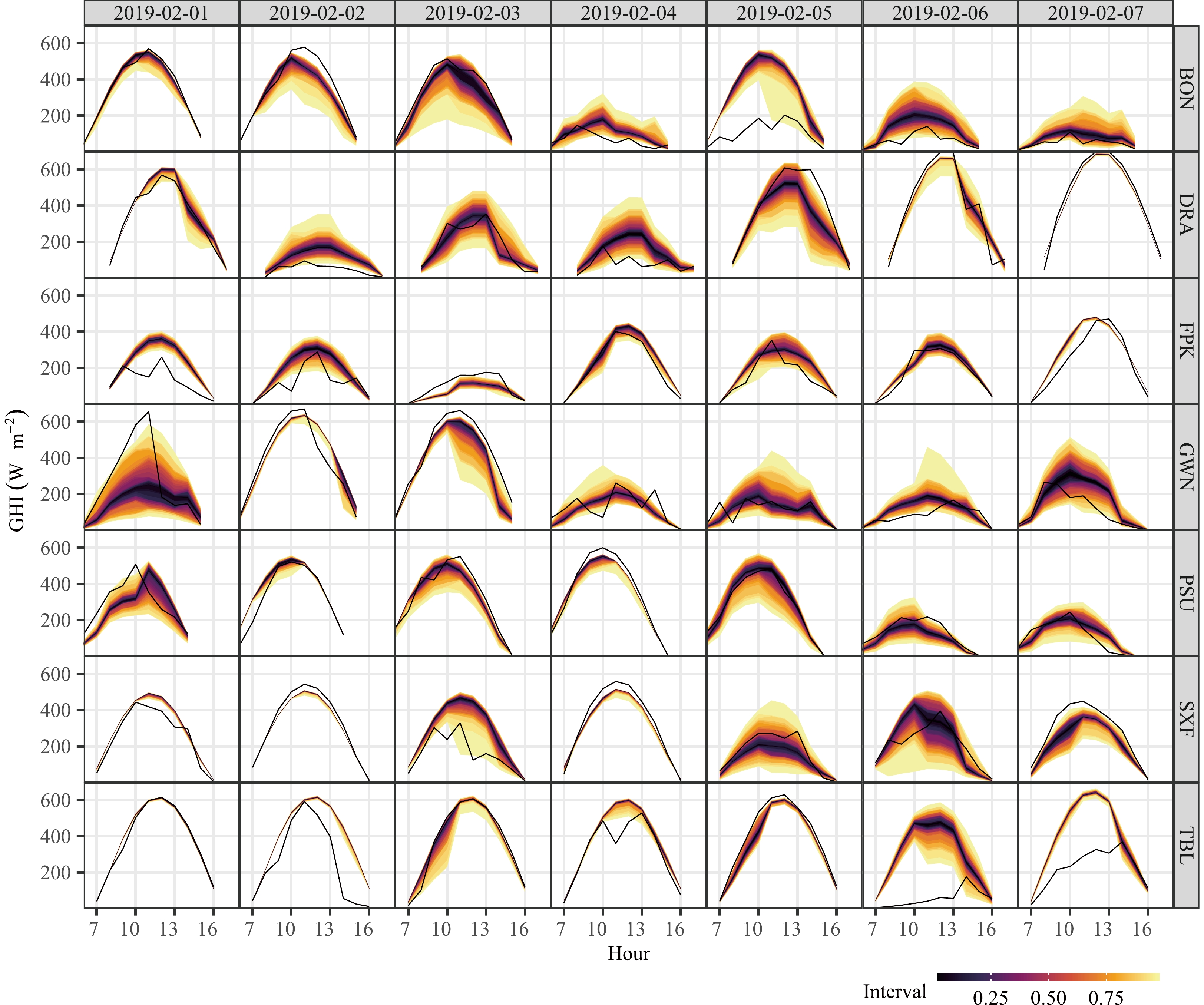
1 The data article by Wang et al. (2022) offers a subset of the archived ENS dataset, which contains ENS GHI forecasts over four years (2017–20) with wide geographical coverage (i.e., most of Europe and the United States). For each day, ensemble GHI forecasts for hours 01:00, 02:00, ..., 23:00, 00:00 (next day) from the 00Z run are used. Figure 1 presents density scatter plots of GHI ensemble means against satellite-derived GHI estimates, at the seven locations of interest. In these plots, brighter colors indicate more points in the neighborhood. A good alignment between the ensemble means and observations is observable at DRA, indicated by clustering around the identity line. This is because DRA has higher clear-sky occurrences and NWP irradiance forecasts are more accurate under clear skies than under cloudy conditions (Yang et al., 2022a). For other stations, more points deviate from the identity lines, indicating that the ensemble means could significantly differ from the truth. Besides, the points of TBL exhibit obvious asymmetry. Since more points are located above the identity line, there are evidently more overestimated ensemble forecasts than underestimated ones. Figure 2 shows 1–24-h-ahead GHI ensembles over the first week of February 2019. It is evident that forecasts are highly accurate under clear skies, e.g., on 7 February 2019 at DRA, but there are also many occasions with ensembles not covering the observations, illustrating the need for calibration.

Figure 1. Scatter plots of GHI ensemble means versus the satellite-derived observations over 2017–20.

Figure 2. Visualization of 1–24-h-ahead GHI ensemble forecasts over the first week of February, 2019. The black solid lines denote the satellite-derived irradiance.
-
Since both the NSRDB and ENS data do not contain gaps, no quality control is required, except for some data transformation and zenith-angle filtering. For time
$ t $ , in order to remove as far as possible the “known” double-seasonal pattern of solar irradiance that is mainly due to the apparent movement of the sun with respect to the observer on Earth, the 50-member ENS GHI, denoted as$ {\mathbf{x}}_{t}=({x}_{t,1}, {x}_{t,2}, \dots ,{x}_{t,50})^{\mathrm{\top }} $ , and satellite-derived NSRDB GHI,$ {y}_{t} $ , are both divided by the clear-sky GHI, so as to obtain ensemble clear-sky index forecasts,$ {\boldsymbol{\pi }}_{t}={({\pi }_{t,1},{\pi }_{t,2}, \dots ,{\pi }_{t,50})}^{\mathrm{\top }} $ , and the clear-sky index verifications,$ {\kappa }_{t} $ (Yang, 2020a, b). According to the recommendations of Yang (2020c), the clear-sky GHI data are obtained from the Copernicus Atmosphere Monitoring Service McClear data service.2 The$ {\boldsymbol{\pi }}_{t} $ and$ {\kappa }_{t} $ are used as the input vector and response variable of the proposed model, respectively; the dimension of each input sample is 50; but the final forecast verification is still performed in irradiance terms, by multiplying the forecast clear-sky index with its clear-sky expectation. Instances with zenith angles larger than 85° are not considered, since clear-sky indexes in low-sun conditions have larger percentage uncertainty but are of little relevance to solar applications (Yang, 2022b). The preprocessed data from 2017 to 2018 are used as the training set, of which the final 20% of data points are used to determine the optimal configuration of the model, and those from 2019 to 2020 are used for true out-of-sample testing; the training set contains 56,689 samples and the test set contains 56,881 samples. -
Denoting a vector of predictors with
$ {\bf{x}}_{t} $ and the response variable with$ {y}_{t} $ , QR focuses on estimating the conditional quantile$ {q}_{t,\tau } $ of$ {Y}_{t} $ at some quantile level$ \tau \in \left[\mathrm{0,1}\right] $ , such that$ P\left({y}_{t}\leqslant {q}_{t,\tau }|{\bf{x}}_{t}\right)=\tau $ . LQR, as the most fundamental form of QR, estimates$ {q}_{t,\tau } $ based on the linear modelwhere
$ \bf{a} $ and$ b $ are regression coefficients that can be estimated by minimizing the sum of quantile losses:where
$ {\hat{q}}_{t,\tau } $ is the estimated conditional quantile for the$ t $ th sample,$ N $ is the number of samples, and$ \rho (\cdot ) $ is the quantile loss, which takes the formTo allow QR-based methods to handle nonlinearity, Taylor (2000) advocated replacing the linear regression with a neural network, and thus coined the name “quantile regression neural network.” Figure 3 shows the structure of a typical QRNN, which is no different in form from a standard multilayer perceptron network (Huber, 1964), in that it consists of an input layer, a hidden layer, and an output layer. The input layer consists of
$ p $ nodes, which are used to receive the input vector$ \mathbf{x}={({x}_{1},{x}_{2},\dots ,{x}_{p})}^{\top} $ . The hidden layer contains$ m $ nodes, which are responsible for generating a feature vector$ \mathbf{h}={({h}_{1},{h}_{2},\dots ,{h}_{m})}^{\top} $ that represents the useful features extracted from$ \mathbf{x} $ . The output layer is used to map the feature vector to the conditional quantile estimates$ {\hat{\mathbf{q}}}=({\hat{q}}_{\tau_1},{\hat{q}}_{\tau_2},\dots, {\hat{q}}_{\tau_l}) $ at$ l $ different quantile levels of interest. The prediction equation of QRNN can be written as
Figure 3. A typical QRNN.
where
$ {\hat{q}}_{{\tau }_{k}} $ is the conditional quantile estimate of quantile level$ {\tau }_{k} $ ,$ \psi (\cdot ) $ and$ \phi (\cdot ) $ are activation functions of the hidden and output layers,$ {\tilde{\alpha }}_{ij} $ is the weight connecting the$ i $ th input node to the$ j $ th hidden node,$ {\alpha }_{jk} $ is the weight connecting the$ j $ th hidden node to the$ k $ th output node, and$ {\tilde{\beta }}_{j} $ and$ {\beta }_{k} $ are the biases of the$ j $ th hidden node and the$ k $ th output node, respectively. The weights and biases of QRNN can be determined by minimizing the quantile loss.3 Quantile crossing occurs very frequently because the output nodes are independent.To address this deficiency of the conventional QRNN, this study proposes NCQRNN, which can solve the quantile crossing problem in its entirety. The overarching design principle of NCQRNN is to add on top of the conventional QRNN structure another hidden layer. The additional layer imposes a non-decreasing mapping between the combined output from nodes of the last hidden layer to the nodes of the output layer, through a triangular weight matrix with positive entries. The new network structure is demonstrated in Fig. 4, which shows without loss of generality a four-layer NCQRNN.

Figure 4. Structure of the proposed NCQRNN.
The 1st hidden layer has the same functionality as in a conventional QRNN, insofar as it is used to extract useful features
$ \mathbf{h} $ from the input, and the activation function of choice is the sigmoid function. After that,$ \mathbf{h} $ is mapped simultaneously to a positive feature vector$ \mathbf{f}={({f}_{1},{f}_{2},\dots ,{f}_{n})}^{\mathrm{\top }}\in {\mathbb{R}}^{n\times 1} $ and a positive weight vector$ \mathbf{w}={({w}_{1},{w}_{2},\dots ,{w}_{n})}^{\mathrm{\top }}\in {\mathbb{R}}^{n\times 1} $ by the added hidden layer (the 2nd hidden layer in this case), whose activation function is the Huber function (Huber, 1964), which is defined aswhere
$ \lambda $ is a small positive constant, which is set to 2−8 (Cannon, 2011; Yang and van der Meer, 2021). Figure 5 plots this function for visualization. Then,$ \mathbf{w} $ is converted to a matrix$ \mathbf{W} $ by a simple transform:
Figure 5. Illustration of the Huber function.
where
$ {\bf{1}}\in {\mathbb{R}}^{l\times 1} $ is a column vector of ones, the symbol “$ \cdot $ ” represents matrix multiplication, the symbol “$ \odot $ ” denotes the Hadamard product (i.e., element-wise or entry-wise product),$ \mathbf{A}\in {\mathbb{R}}^{n\times l} $ is a matrix with lower triangular elements of zeros, in which all elements of the last column are 1, and the number of 1s in the previous column is one fewer than that in the preset column. Finally, conditional quantile estimates can be obtained viaFor instance, if one sets
$ n=l+1 $ ,$ \mathbf{A}\in {\mathbb{R}}^{(l+1)\times l} $ can be expressed as$ \mathbf{W} $ can be expressed asand the conditional quantile estimates can be obtained via
To make
$ {\hat{q}}_{{\tau }_{1}} $ not equal to zero, the elements of the first column in$ \mathbf{W} $ cannot all be zero, which is equivalent to$ n > l $ . That is,$ n $ can be set to any value larger than$ l $ .The NCQRNN changes the way that the output layer and the last hidden layer in the QRNN are connected; the next output node connects with one more hidden node than the previous output node. Due to the structure of
$ \mathbf{W} $ , the prediction of the next quantile level equals the sum of predictions of the previous quantile level and a weighted hidden node feature. Since both$ \mathbf{f} $ and$ \mathbf{w} $ are positive—due to the use of Huber loss as the activation function—the output values are monotonically increasing, and the crossing problem is thus solved. Compared with previous QR methods with non-crossing quantiles, NCQRNN needs no inequality constraints and is therefore very flexible. This new non-crossing quantile design can be integrated with many other network structures, such as an Elman neural network (ENN), a convolutional neural network (CNN), a long short-term memory (LSTM) network, a stacked autoencoder, or a deep belief network, by replacing the 1st hidden layer in the present network structure with the corresponding shallow or deep network structures. Stated differently, for any given network structure, as long as an additional layer in the style of$ \mathbf{f} $ and$ \mathbf{w} $ is added between the last hidden layer and the output layer, non-crossing quantiles can be achieved. In what follows, three variants of NCQRNN are introduced. -
In the NCQRNN described in section 3.1, both weights and features of the 2nd hidden layer need to be generated. In order to reduce the parameters of the model, the first variant of NCQRNN only generates the features
$ \mathbf{f} $ , and the$ \mathbf{w} $ is set to be the same as$ \mathbf{f} $ . This approach also solves the quantile crossing problem, and the obtained conditional quantile estimations are given byFor convenience, this variant is referred to as NCQRNN-I henceforth.
-
In NCQRNN,
$ \mathbf{w} $ is obtained based on$ \mathbf{h} $ . Since$ \mathbf{h} $ varies with the input$ \mathbf{x} $ ,$ \mathbf{w} $ also depends on$ \mathbf{x} $ . Similar to the motivation behind NCQRNN-I, i.e., to reduce the parameters of the model, it is possible to set$ \mathbf{w} $ as a constant vector, i.e.,$ \mathbf{w} $ is the same for all test samples after the model training. For convenience, this variant is referred to as NCQRNN-II. -
The NCQRNN shown in Fig. 4 is a four-layer model that has two hidden layers, and the 1st hidden layer is used to capture features of the raw input. However, even with the 1st hidden layer removed, non-crossing QR can still be achieved. In this case, input vectors would be directly mapped to
$ \mathbf{w} $ and$ \mathbf{f} $ . This variant is referred to as NCQRNN-III. -
Pinson et al. (2007) emphasized that the quality of probabilistic forecasts can be divided into three properties: calibration, sharpness, and resolution; this view was reiterated by Lauret et al. (2019), but noting that among the three properties, the calibration and sharpness are complementary and sufficient in gauging the goodness of probabilistic forecasts. Whereas calibration focuses on statistical consistency between observations and forecasts, sharpness is concerned with the concentrations of the probabilistic forecasts (Gneiting and Katzfuss, 2014). One should note that both properties can be analyzed quantitatively and qualitatively: quantitative analyses would result in numerical scores, whereas qualitative analyses employ graphical diagnostic tools to evaluate various properties (Lauret et al., 2019; Yagli et al., 2020). In what follows, the forecast verification is achieved largely on this basis. However, instead of following entirely the procedure advocated by Lauret et al. (2019), the CORP reliability diagram, which stands for “Consistent, Optimal, Reproducible, and Pool-adjacent-violators (PAV) algorithm,” is additionally used, conforming to the latest advance and recommendations in the field of statistics in evaluating the reliability of probabilistic forecasts (Dimitriadis et al., 2021).
-
The commonly used metrics of calibration and sharpness are prediction interval coverage probability (PICP) and prediction interval average width (PIAW), respectively. PICP represents the actual coverage rate of PIs with a nominal coverage rate of
$ \alpha $ , which is defined aswhere
$ {L}_{t}^{\alpha } $ and$ {U}_{t}^{\alpha } $ denote the lower and upper bounds of the PI of the$ t $ th sample. The PICP of calibrated predictive distributions should be close to the nominal coverage rate (Lauret et al., 2019). On the other hand, PIAW assesses the width of PIs, which is defined asA small PIAW indicates concentrated predictive distributions (Yang et al., 2020). The paradigm of good probabilistic forecasting is to maximize the sharpness while maintaining a coverage rate close to the nominal coverage rate (Gneiting et al., 2007; Yang et al., 2020). As such, the two above metrics must be used together.
Aside from evaluating calibration and sharpness individually, there are also composite scores that can assess both properties simultaneously. For instance, CRPS is one of those composite scores that have many amenable statistical properties; for a predictive distribution
$ {\hat{F}}_{t}\left(\cdot \right) $ and a verification$ {y}_{t} $ , its CRPS is (Hersbach, 2000)where
$ {\bf{1}}\left(\cdot \right) $ is the Heaviside step function. CRPS inherits the unit of the quantity that it evaluates. On top of using CRPS itself, Murphy (1988) suggested that skill scores should also be reported when forecast models are compared. A skill score represents the relative improvement in the performance of the model of interest with respect to a reference model. Following that definition, the CRPS skill score (CRPSS) iswhere
$ {\mathrm{C}\mathrm{R}\mathrm{P}\mathrm{S}}_{\mathrm{m}\mathrm{o}\mathrm{d}\mathrm{e}\mathrm{l}} $ and$ {\mathrm{C}\mathrm{R}\mathrm{P}\mathrm{S}}_{\mathrm{r}\mathrm{e}\mathrm{f}\mathrm{e}\mathrm{r}\mathrm{e}\mathrm{n}\mathrm{c}\mathrm{e}} $ are CRPS values of the model of interest and the standard of reference, respectively. Yang (2019b) proposed a new reference model called the complete-history persistence ensemble (CH-PeEn), which is essentially a form of conditional climatology that can overcome issues of the sample-dependence of the traditional persistence ensemble. CH-PeEn is therefore used as the standard of reference in this study, as also endorsed and recommended by Gneiting et al. (2023), Doubleday et al., (2020), and Lauret et al. (2019) in their seminal reviews on probabilistic forecast benchmarking. -
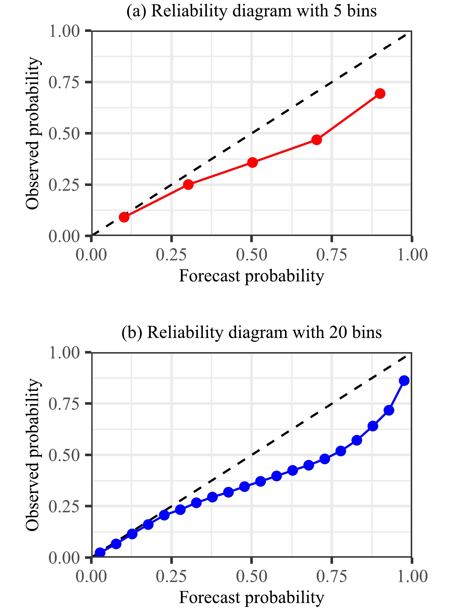
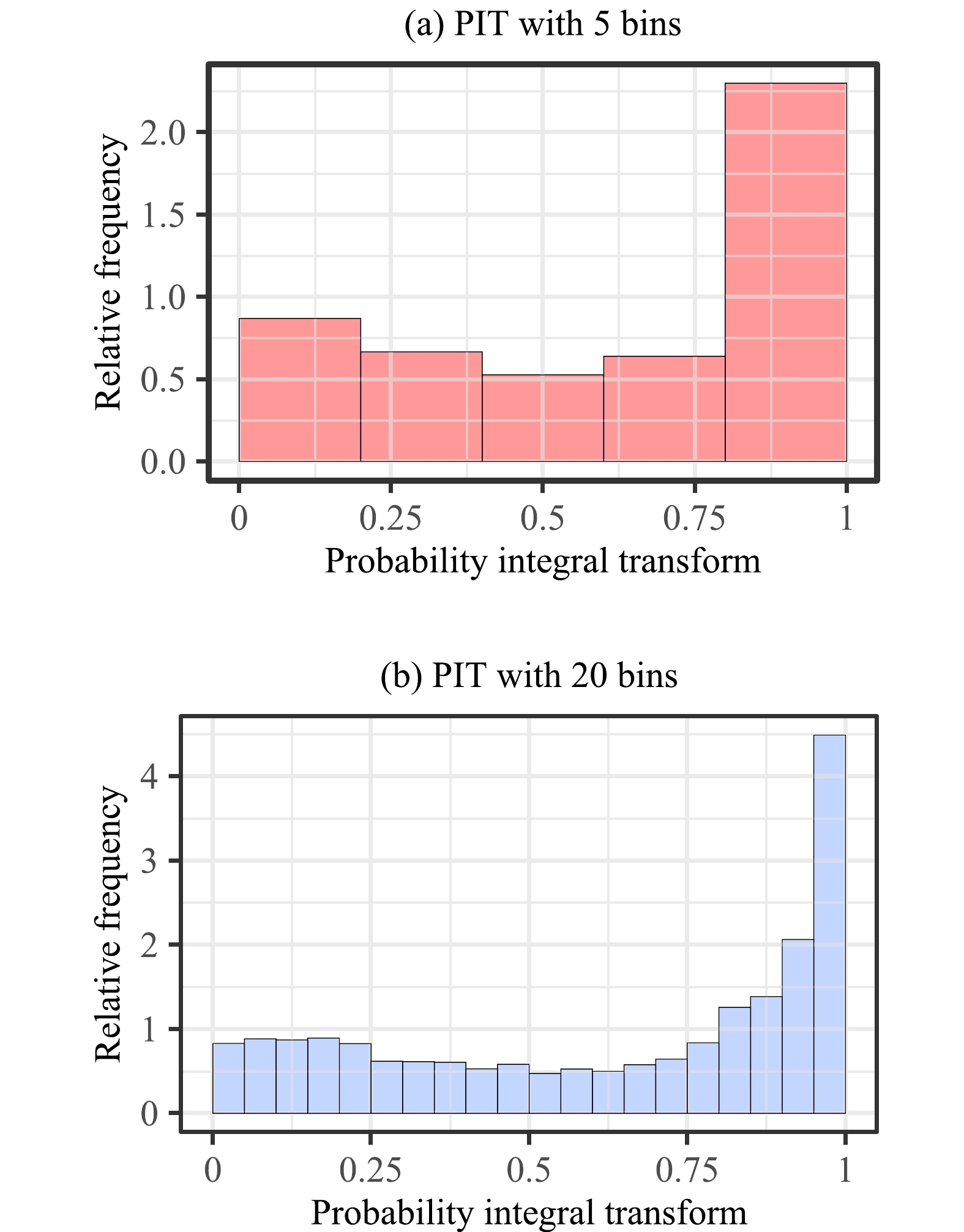
Calibration and sharpness can be visually assessed by graphical diagnostic tools (Lauret et al., 2019; Yagli et al., 2020). The reliability diagram and PIT histogram have hitherto been the two most popular calibration evaluation tools in the weather forecast verification community (Lauret et al., 2019). The reliability diagram checks whether observed and forecast probabilities are close, and the PIT histogram verifies whether observations can be seen as random samples of the predictive probability distributions (Gneiting and Raftery, 2007; Pinson et al., 2010). However, both tools require manual binning, which affects the shape of plots and therefore the eventual judgment. For instance, Figs. 6 and 7 show the reliability diagrams and PIT histograms of calibrated quantile forecasts of the gradient-boosted regression tree (GBRT) at DRA over 2019–20 (experimental details of the calibration are provided below). The shape of the plot changes with the number of bins. This means that the evaluation results are not only dependent on the forecasts, but are also influenced by the parameters of evaluation tools, which is an undesirable trait (Lauret et al., 2019).

Figure 6. Reliability diagrams with 5 and 20 bins for post-processed quantile forecasts of GBRT at DRA over 2019–20.

Figure 7. Probability integral transform histograms with 5 and 20 bins for post-processed quantile forecasts of GBRT at DRA over 2019–20.
To solve this problem, Dimitriadis et al. (2021) developed the CORP reliability diagram. CORP first estimates the conditional event probability (CEP) based on nonparametric isotonic regression and the PAV algorithm, and bins are determined optimally and automatically. Then, it plots the estimated CEP versus the forecast probability to show the reliability. Different from the traditional reliability diagram, the CORP reliability diagram is non-decreasing—decreasing estimates are counterintuitive, which are routinely viewed as artifacts and dismissed by practitioners (Dimitriadis et al., 2021). CORP is applicable to both continuous and discrete forecasts, and the forecasts are reliable if the diagram aligns well with the diagonal. The reader is referred to Dimitriadis et al. (2021) for more technical details regarding CORP.
-
This study employs a total of 13 benchmark models with diverse predicting mechanisms to test the performance of the proposed approach. The 13 benchmarks consist of 1 naïve reference model, 2 parametric models, and 10 nonparametric models, among which some may be considered as state-of-the-art models. As mentioned earlier, CH-PeEn (Yang, 2019b) is to be used as the standard of reference, mainly for CRPSS calculation. The parametric models include EMOS (Gneiting et al., 2005) and Gaussian-process regression (GPR; Seeger, 2004), which both assume that the response variable has a normal distribution. The nonparametric models include analog ensemble (AnEn; Yang, 2019c), LQR, QRF, quantile-loss-based GBRT, QRNN, quantile-loss-based ENN (QRENN), quantile-loss-based one-dimensional CNN (QRCNN), quantile-loss-based LSTM (QRLSTM), an NN-based non-crossing method Bernstein quantile network (BQN; Bremnes, 2020) with minor adaptations by Schulz and Lerch (2022), and the positive-increment based non-crossing approach (QRPI). Whereas the prediction mechanisms of other benchmarks are either self-explanatory or acquainted, it should be just clarified that, in QRPI, the back-propagation neural network outputs quantiles of the 1st quantile level and positive increments of two adjacent quantile levels with the Huber function, and then all quantiles are obtained by accumulating positive increments from quantiles of the 1st quantile level. Since increments are positive, the predicted quantiles are monotonically increasing.
In terms of setup, CH-PeEn selects the historical clear-sky indexes at the same time of day as the forecast time stamp (e.g., if the time of day is “HH:00,” all data at time “HH:00” in 2017 and 2018 are selected), thus forming an ensemble of the clear-sky index, which is multiplied with the clear-sky expectation at the forecast hour to generate the ensemble GHI forecasts (Yang, 2019b). AnEn compares the ensemble at the forecast time stamp to all ensembles over 2017–18, and the GHI observations corresponding to the M-best ensembles are selected to form an ensemble, where M is set to be equal to the number of quantile levels used in other quantile-based models.
For those benchmark models that issue quantiles, a total of 199 quantile levels {0.005, 0.01, …, 0.99, 0.995} are selected to fully characterize the underlying distribution; that is, l = 199. The ensemble NWP forecasts at each time stamp are first sorted, because the perturbed forecasts are exchangeable, so it is incorrect to think of forecasts with the same member index but from different runs as those from a typical model (Vannitsem et al., 2018; Bremnes, 2020; Schulz and Lerch, 2022; Mayer and Yang, 2023b); this sort of mistake is commonly committed in the literature (e.g., Sperati et al., 2016). Since QRCNN and QRLSTM are temporal-feature-based models, their input sample at
$ t $ contains$ {\boldsymbol{\pi }}_{t} $ and$ {n}_{\mathrm{l}\mathrm{a}\mathrm{g}} $ lagged ensemble clear-sky index forecasts, while the input of other models is just$ {\boldsymbol{\pi }}_{t} $ . Additionally, for QRCNN and QRLSTM, the search range of lag$ {n}_{\mathrm{l}\mathrm{a}\mathrm{g}} $ is {10, 20, 30}.On parameter estimation for EMOS, since each ensemble member represents the future GHI in an equally probable fashion, the weights
$ \{{m}_{1}, \dots ,{m}_{p}\} $ of its ensemble members should be identical, i.e.,$ {m}_{1}=\dots ={m}_{p}=1/p=0.02 $ (Wang et al., 2022), and the remaining model parameters, i.e., the linear coefficients adjusting the variance, are estimated via the strategy of minimizing CRPS; all these are well known. For QRNN, QRENN, QRCNN, QRLSTM, QRPI, BQN, and NCQRNN, the models are constructed with Keras, and the model parameters are optimized using the Adam optimization algorithm by minimizing the Huber quantile loss (Wang et al., 2019):The training epoch, batch size and learning rate are set to 1000, 3000 and 0.002, respectively (Zou et al., 2022). The settings of most model hyperparameters are determined based on using a grid search. Table 2 presents the search ranges of different hyperparameters. The model hyperparameters of BQN are set according to Schulz and Lerch (2022), i.e., BQN consists of three hidden layers with neurons of 96, 48, and 24, respectively, and the degree of the polynomials is set to 12. The other benchmark models are implemented in R language.
Model Layer Filter/Neuron Kernel size Activation QRNN Hidden layer 1 {10,20, … ,150} – Sigmoid QRENN Hidden layer 1 {10,20, … ,150} – Sigmoid QRCNN Convolutional layer 1 {8,16,32,64} {2,3,4} ReLU Convolutional layer 2 {8,16,32,64} {2,3,4} ReLU Convolutional layer 3 {8,16,32,64} {2,3,4} ReLU QRLSTM LSTM {5,10,20,30} – Tanh QRPI Hidden layer 1 {10,20, … ,150} – Sigmoid NCQRNN Hidden layer 1 {5,10,20,30} – Sigmoid Hidden layer 2 {200,210,220} – Huber function Table 2. Search ranges of different hyperparameters.
-
The calibrated probabilistic forecasts can be obtained by feeding the validation samples into the trained models. Tables 3 to 6 present the performance of the raw ensemble NWP forecasts and various versions of calibrated forecasts, based on the four aforementioned evaluation metrics, at seven stations, over two years. Consolidating the observations made from those tables, the following conclusions can be drawn:
Station Raw GPR EMOS AnEn LQR QRF GBRT QRNN QRENN QRCNN QRLSTM QRPI BQN NCQRNN PICP with 85% nominal coverage probability (%) BON 33.38 84.08 83.46 83.54 82.71 79.13 77.27 83.42 84.23 83.30 81.51 82.60 81.97 77.58 DRA 16.30 89.29 81.98 79.66 79.36 75.22 62.87 81.24 77.10 83.45 78.01 87.66 86.08 81.15 FPK 30.71 87.41 86.14 84.04 85.02 79.45 75.36 84.33 85.66 86.30 85.44 86.64 88.95 86.70 GWN 31.03 84.97 81.44 82.74 82.70 79.00 74.29 79.60 85.91 85.38 84.27 90.13 84.95 83.39 PSU 36.23 85.59 86.05 83.60 83.91 78.74 74.97 87.02 83.31 86.80 83.07 94.03 87.71 85.51 SXF 30.71 85.10 84.68 83.37 83.69 77.47 77.36 85.78 81.71 84.35 83.41 93.65 88.02 83.90 TBL 31.00 89.34 87.20 85.49 85.21 80.76 80.57 84.58 84.34 91.01 80.70 95.68 86.86 89.18 Mean 29.91 86.54 84.42 83.21 83.23 78.54 74.67 83.71 83.18 85.80 82.34 90.06 86.36 83.92 PICP with 90% nominal coverage probability (%) BON 36.73 88.35 87.19 88.80 87.86 84.19 84.53 88.01 89.43 88.31 87.30 89.74 87.00 84.59 DRA 18.19 91.84 85.44 85.41 85.28 80.65 72.79 84.54 85.41 88.06 84.57 95.69 92.16 87.69 FPK 34.30 92.09 89.53 88.96 90.38 84.35 83.56 89.88 90.87 90.87 90.46 91.58 93.40 91.31 GWN 34.43 88.96 85.64 88.12 87.83 84.05 82.06 89.35 90.25 90.06 88.79 93.54 88.70 89.26 PSU 40.30 90.08 89.48 89.31 88.78 84.27 83.47 92.03 88.42 91.14 88.92 97.49 92.03 90.68 SXF 34.05 89.71 88.48 88.83 88.64 82.86 84.11 89.95 89.48 90.16 89.80 97.14 91.23 89.89 TBL 34.29 92.48 90.14 90.37 90.65 85.77 85.68 89.91 89.78 94.31 87.76 97.36 94.02 92.16 Mean 33.18 90.50 87.99 88.54 88.49 83.73 82.31 89.10 89.09 90.42 88.23 94.65 91.22 89.37 PICP with 95% nominal coverage probability (%) BON 41.45 93.02 91.13 93.85 93.75 89.94 91.66 94.99 95.01 93.74 93.34 97.15 91.24 92.38 DRA 20.48 94.56 89.00 92.24 92.04 87.47 83.56 92.60 92.23 93.22 92.19 98.36 95.90 93.06 FPK 38.24 95.68 92.99 94.24 95.21 89.57 90.96 95.48 95.76 95.65 95.54 95.42 95.98 95.88 GWN 39.00 92.77 90.01 94.04 93.33 89.40 88.25 93.43 94.38 94.61 93.98 97.89 91.55 94.63 PSU 45.47 94.48 92.95 94.60 94.24 90.10 91.97 94.91 95.39 95.84 94.55 99.37 94.98 96.19 SXF 38.69 93.84 92.49 94.21 94.72 88.95 90.31 96.45 94.73 95.35 94.99 98.60 93.28 94.17 TBL 39.18 95.74 92.89 95.04 95.14 91.06 91.47 95.48 95.26 97.17 93.89 98.94 96.46 96.74 Mean 37.50 94.30 91.64 94.03 94.06 89.50 89.74 94.76 94.68 95.08 94.07 97.96 94.2 94.72 Table 3. PICP (%) with different nominal probabilities of raw ensembles, 12 post-processing benchmark models (section 4.2), as well as the proposed NCQRNN (section 3.1), computed using the entire test set. Row-wise best results are in bold.
(1) Post-processing can effectively improve the calibration of ensemble NWP forecasts. As shown in Table 3, the mean PICPs at 85%, 90% and 95% nominal coverage rates of those raw ensemble NWP forecasts are 29.91%, 33.18% and 37.5%, respectively, which are significantly lower than the nominal probabilities and PICPs of other models, indicating that the raw ensemble NWP forecasts are under-dispersed. The under-dispersion is echoed in Table 4, in which the PIAWs of raw ensembles at three nominal coverage rates are shown to be much lower than those of post-processed forecasts, revealing that raw ensembles are overly sharp—recall again that sharpness is not useful unless the forecasts are calibrated.
Station Raw GPR EMOS AnEn LQR QRF GBRT QRNN QRENN QRCNN QRLSTM QRPI BQN NCQRNN PIAW with 85% nominal coverage probability (%) BON 130.34 293.09 264.21 290.15 284.55 276.08 268.84 286.34 285.34 263.19 263.92 294.59 299.75 287.73 DRA 58.73 192.37 160.45 153.05 160.51 150.59 137.07 160.61 151.76 176.72 153.64 195.83 219.01 157.65 FPK 109.99 306.30 276.81 302.19 306.34 283.20 282.46 297.01 304.03 290.78 292.83 308.76 340.49 301.90 GWN 130.16 294.35 242.16 265.95 271.88 256.47 250.34 254.04 276.87 263.04 262.86 399.04 274.40 268.69 PSU 141.91 314.67 296.04 309.44 311.79 293.30 290.85 321.24 304.17 303.87 300.48 447.93 324.11 305.51 SXF 125.51 302.85 276.98 296.83 306.48 274.69 269.75 310.12 295.57 301.51 289.92 376.26 310.97 302.70 TBL 102.72 341.53 296.56 322.17 326.86 303.05 327.81 333.85 322.60 330.79 317.01 417.57 361.99 334.97 Mean 114.19 292.17 259.03 277.11 281.20 262.48 261.02 280.46 277.19 275.70 268.67 348.57 304.39 279.88 PIAW with 90% nominal coverage probability (%) BON 146.94 334.89 301.90 330.92 326.92 308.41 312.05 330.00 329.87 306.43 306.46 350.50 349.58 325.45 DRA 66.70 219.81 183.34 180.71 192.74 174.92 168.88 185.11 184.88 213.66 185.82 312.82 277.52 209.89 FPK 123.93 349.98 316.29 342.88 353.76 316.77 332.07 338.09 353.86 337.70 335.75 362.32 402.83 348.13 GWN 147.23 336.33 276.69 309.08 313.25 290.03 287.41 322.83 316.15 312.33 304.70 470.01 318.62 320.20 PSU 159.41 359.56 338.26 347.17 349.98 325.87 329.89 365.58 339.11 344.46 340.46 537.88 364.83 347.15 SXF 141.34 346.05 316.48 341.47 346.29 308.00 307.27 349.34 350.51 346.51 337.33 470.44 352.74 354.37 TBL 115.87 390.24 338.86 364.80 382.23 337.68 363.60 376.28 371.70 385.46 359.99 474.51 432.15 374.21 Mean 128.77 333.84 295.97 316.72 323.60 294.53 300.17 323.89 320.87 320.94 310.07 425.50 356.90 325.63 PIAW with 95% nominal coverage probability (%) BON 168.97 399.05 359.73 385.25 387.88 351.41 370.67 394.23 394.32 376.99 371.13 447.05 410.52 393.68 DRA 77.79 261.92 218.46 239.18 251.26 214.36 215.14 242.44 245.81 269.47 245.46 444.38 352.08 263.74 FPK 143.39 417.03 376.89 402.12 424.86 359.28 417.91 416.79 429.50 411.07 411.27 429.28 481.33 412.31 GWN 169.82 400.76 329.70 375.53 380.53 337.11 333.24 380.98 385.55 381.09 381.83 575.73 373.63 397.78 PSU 183.48 428.44 403.06 404.59 409.15 367.77 383.81 419.68 409.85 404.84 397.22 697.47 411.19 414.20 SXF 163.05 412.35 377.11 402.26 407.67 353.08 356.03 420.11 406.25 409.32 401.98 572.25 400.41 402.07 TBL 133.91 465.00 403.78 428.43 446.64 381.78 419.40 447.36 450.48 460.52 433.17 549.39 519.38 447.78 Mean 148.63 397.79 352.68 376.77 386.86 337.83 356.60 388.80 388.82 387.61 377.44 530.79 421.22 390.22 Table 4. As in Table 3 but for PIAW (%).
(2) Nonparametric models generally perform better than parametric models, except for QRF and GBRT, which have the worst overall performance. Although the PIAWs of these two models at 85%, 90% and 95% nominal coverage rates are lower than other post-processing models, their PICPs are also the lowest, indicating insufficient coverage. Recall that sharpness only should be appraised when reliability is met. In terms of the comprehensive quality of probabilistic forecasts, the mean CRPSSs of QRF and GBRT are 32.75% and 32.91%, respectively, which show the slightest improvement among all the post-processing models. Besides QRF and GBRT, the mean CRPSSs of GPR and EMOS are 27.19% and 32.84%, which are lower than all other nonparametric models. The reason can be attributed to the fact that the distribution of clear-sky index or irradiance is rarely normal (Yang, 2022a).
4 (3) Shallow neural network models, surprisingly, perform better than those deep-learning models in terms of the calibration of ensemble NWP forecasts. More specifically, the CRPSSs of QRNN, QRENN, NCQRNN, QRCNN, and QRLSTM are 35.62%, 35.74%, 36.20%, 34.89%, and 35.42%, respectively. Shallow neural network models (QRNN, QRENN, NCQRNN) achieve greater promotion than deep-learning models (QRCNN, QRLSTM) in terms of skill score. The reason for this observation is discussed in section 5.2.
(4) The newly proposed model has the best post-processing performance while avoiding crossing. As shown in Table 6, NCQRNN performs the best at all stations except BON. The overall CRPSS of NCQRNN is also the highest among all the models considered. In terms of the crossing problem, this study calculates the average number of crossings for the quantile-regression type of models, which is defined as
Station Raw GPR EMOS AnEn LQR QRF GBRT QRNN QRENN QRCNN QRLSTM QRPI BQN NCQRNN CRPSS (%) BON 32.13 32.03 37.47 40.05 39.27 37.40 37.41 39.88 40.40 38.88 39.72 39.66 37.64 40.04 DRA 9.78 23.33 31.13 35.17 32.11 31.84 31.91 35.01 33.39 32.64 33.59 31.82 25.54 35.19 FPK 19.78 21.45 27.71 30.34 28.77 26.30 25.72 30.61 30.11 30.81 30.21 28.73 27.34 31.10 GWN 33.96 34.01 39.99 42.79 40.89 40.07 37.34 41.90 42.52 41.43 42.77 28.04 39.82 42.92 PSU 32.27 33.90 37.31 39.97 38.37 37.20 38.84 39.46 40.00 38.65 39.64 20.55 37.64 40.19 SXF 24.61 25.66 31.12 33.47 33.11 30.75 32.35 34.05 34.12 33.10 33.63 31.47 32.81 34.10 TBL 17.96 19.92 25.15 29.12 27.96 25.66 26.82 28.40 29.63 28.73 28.37 27.53 24.06 29.89 Mean 24.36 27.19 32.84 35.84 34.35 32.75 32.91 35.62 35.74 34.89 35.42 29.69 32.12 36.20 Table 6. As in Table 3 but for CRPSS (%).
where
$ \mathrm{s}\mathrm{i}\mathrm{g}\mathrm{n}(\cdot ) $ is the sign function, and$ c $ denotes the average number of quantiles that are higher than the following quantiles for a sample. If the quantiles of two arbitrary adjacent quantile levels cross,$ c $ is equal to$ l-1 $ , that is$ c=198 $ in this study. From Table 7, it is evident that NCQRNN entirely solves the crossing problem, as$ c=0 $ at all stations. However, for other models, except QRPI and BQN, the mean crossing numbers are between 30 and 69, showing that the crossing problem happens with a probability of 15.15%–34.85%. In addition, since only quantile crossing of two adjacent quantile levels is considered here, the actual number of crossings will be larger. Although QRPI and BQN are also free of crossing, they perform significantly worse than NCQRNN in terms of CRPS and CRPSS.(5) Calibrated forecasts under cloudy-sky conditions are more reliable. Figure 8 shows the CORP reliability diagrams of raw and post-processed forecasts issued by some selected models. (Only eight sets of forecasts are selected because the colorblind palette only has eight colors, beyond which the diagrams may become illegible.) The diagrams of NCQRNN are closer to the diagonals than those of other models in most cases, which indicates that the forecasts of the proposed model are more reliable. To investigate the post-processing performance under different sky conditions, the testing samples from all stations are divided into overcast, clear-sky, and cloudy-sky conditions, and then the CORP diagrams of calibrated forecasts are plotted for each of the three sky conditions, respectively. According to Fig. 9, it can be seen that the diagrams of calibrated forecasts for cloudy-sky conditions are closer to the diagonal compared to those of clear-sky and overcast conditions. Therefore, it can be concluded that post-processed forecasts of cloudy weather are more reliable.
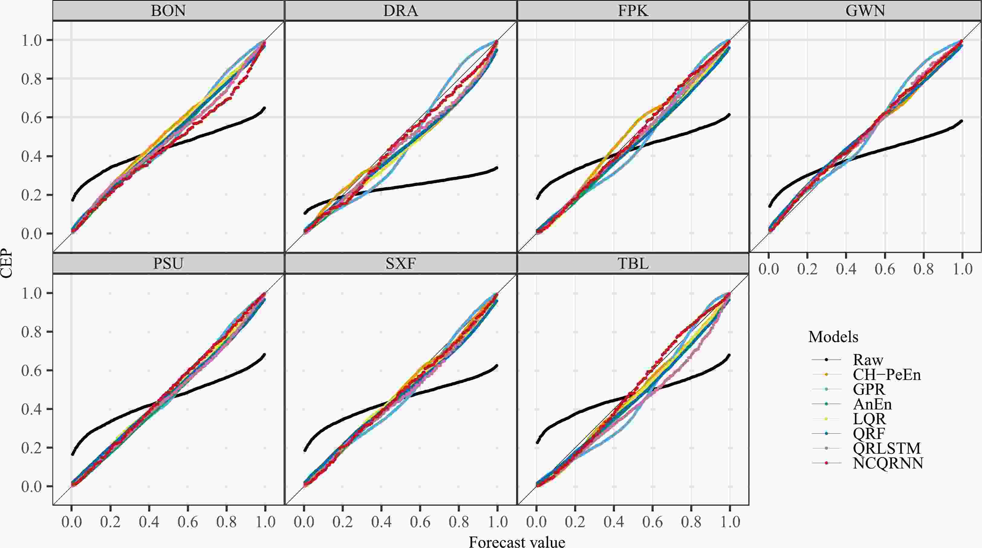
Figure 8. CORP reliability diagrams of selected post-processed forecasts over 2019 to 2020.

Figure 9. CORP reliability diagrams of post-processed forecasts under three sky conditions from all stations over 2019−20.
(6) The predictive performance of various calibration methods is consistent across stations, and is generally independent of the irradiance regimes at different stations. Figure 10 shows CRPSSs of different models at different stations. The seven stations can be divided into three categories based on the overall CRPSSs: stations with large improvement (BON, GWN, PSU), stations with medium improvement (DRA, SXF), and stations with small improvement (TBL, FPK). According to Yang (2022a), there are substantial differences in the predictability of solar irradiance across SURFRAD stations, which determines how much improvement one can potentially achieve through calibration. However, independent of predictability, the performance ranking of various models at each station is quite consistent, as shown by the shapes of the histograms.

Figure 10. CRPSSs of various post-processing models over 2019–20. Brighter colors indicate higher values.
Figure 11 shows the PIs of the proposed model at nominal coverage rates of 85%, 90%, and 95%. Most of the observations fall within the PIs, and PIs could effectively respond to the observations, showing good resolution—recall that resolution generally suggests the ability to issue different forecasts for different forecasting situations. Compared to Fig. 2, the under-dispersion problems of raw ensembles are solved.

Figure 11. Several (50%, 90%, and 95%) central PIs of the proposed NCQRNN, at seven stations, over the first 300 hours in January 2019. The RMSEs for the means of post-processed forecasts and ensemble NWP forecasts are, however, calculated based on the entire test set.
Station Raw GPR EMOS AnEn LQR QRF GBRT QRNN QRENN QRCNN QRLSTM QRPI BQN NCQRNN CRPS (W m−2) BON 58.88 58.97 54.25 52.01 52.69 54.31 54.30 52.16 51.71 53.03 52.30 52.35 54.10 52.02 DRA 40.69 34.58 31.06 29.24 30.62 30.74 30.71 29.31 30.04 30.38 29.95 30.75 33.58 29.23 FPK 56.48 55.31 50.90 49.05 50.15 51.89 52.30 48.86 49.21 48.72 49.14 50.18 51.16 48.51 GWN 58.70 58.65 53.34 50.85 52.54 53.27 55.69 51.64 51.09 52.06 50.87 63.96 53.49 50.73 PSU 61.43 59.95 56.86 54.45 55.90 56.96 55.47 54.91 54.42 55.64 54.75 72.06 56.56 54.25 SXF 60.61 59.77 55.38 53.49 53.78 55.68 54.39 53.02 52.97 53.79 53.36 55.10 54.02 52.98 TBL 63.33 61.81 57.78 54.71 55.61 57.38 56.49 55.27 54.32 55.01 55.29 55.94 58.62 54.12 Mean 57.16 55.58 51.37 49.11 50.18 51.46 51.34 49.31 49.11 49.80 49.38 54.33 51.65 48.83 Table 5. As in Table 3 but for CRPS (W m−2).
Station LQR QRNN QRENN QRCNN QRLSTM QRPI BQN NCQRNN Average number of quantile crossings BON 30 63 70 62 35 0 0 0 DRA 29 71 74 65 50 0 0 0 FPK 29 59 66 59 37 0 0 0 GWN 31 68 71 66 49 0 0 0 PSU 31 61 70 57 37 0 0 0 SXF 29 63 68 66 41 0 0 0 TBL 31 60 63 49 39 0 0 0 Mean 30 64 69 61 41 0 0 0 Table 7. Average number of quantile crossings for different QR methods over 2019–20. Quantile crossing instances are counted for each forecast time stamp, and then averaged. Since there are 199 quantiles, the number 30 means that the crossing problem happens with a probability of 30 / 198 = 15.15%. Row-wise best results are in bold.
-
Three variants of NCQRNN—namely, NCQRNN-I, NCQRNN-II, and NCQRNN-III—are proposed in sections 3.2 to 3.4. Figure 12 presents the CRPSSs of NCQRNN and its three variants. It can be seen that the performance of NCQRNN-I is close to, but still not as good as, NCQRNN. NCQRNN-III ranks next to NCQRNN-I, indicating that the 1st hidden layer can help improve the forecast performance. This confirms that the 1st hidden layer can capture important features of the input, which helps generate better weights and input features for subsequent layers of the network. NCQRNN-II performs worst, showing that it is not beneficial to use the same weights for all samples. Due to the changing irradiance regimes, ensemble NWP forecasts made for these regimes also have different characteristics, and thus the calibration weights should respond to those accordingly.
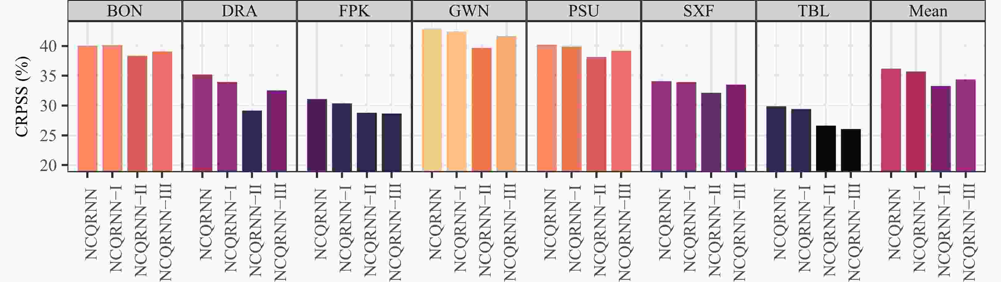
Figure 12. CRPSSs of NCQRNN and its three variants over 2019–20. Brighter colors indicate higher values.
-
As shown in Fig. 11, the RMSEs of the means of calibrated quantile forecasts are close to those of ensemble NWP forecasts at most stations, indicating that the calibration is achieved mainly by improving the dispersion of raw ensembles, whereas the conditional bias in forecasts is not deliberately attended to. It should be highlighted that this “deficiency” is not specific to the present models, but is general for all quantile-based models—QR minimizes the pinball loss, which is unrelated to the bias in mean of predictive distribution. This property has been widely reported in the literature, and various procedures have been proposed to enhance QR with bias correction ability (e.g., Wei and Carroll, 2009; Guo et al., 2021). However, motivated by the scatter plots shown in Fig. 13, applying simple linear corrections to the mean values of predictive distributions seems sufficient.

Figure 13. Scatter plots of the means of post-processed quantile forecasts versus satellite-derived irradiance observations at an arbitrarily selected station (SXF) over 2019–20.
Indeed, Fig. 13 shows the scatter plots of the means of quantile forecasts of all models versus satellite-derived GHI on test sets at station SXF, with brighter colors suggesting a higher concentration of data points in the neighborhood. It can be seen that the means of calibrated forecasts exhibit similar error behaviors, insofar as the models tend to overestimate when observations are low and underestimate when observations are high, which could be largely attributable to the misidentification of sky conditions. This phenomenon suggests that the P2P calibration of ensemble NWP forecasts does not eliminate conditional forecast biases, which certainly affects the forecasting performance. In this regard, the question of whether removing biases prior to calibration must be addressed. This section first tries to reduce the conditional forecast biases from two aspects: historical observations and historical raw ensembles. After that, in order to verify whether fewer ensemble members reduce the forecast performance while reducing the computational cost, the forecasts with different input dimensions are discussed.
-
This study considers four methods that leverage historical observations to improve the calibration performance. The first method corrects
$ {\bf{x}}_{t} $ based on the observation of the previous forecast instance, which is expressed as follows:where
$ {{\bf{x}}'_{t}} $ denotes the corrected ensemble NWP forecasts at$ t $ , and$ {\bar{x}}_{t} $ is the mean value of$ {\bf{x}}_{t} $ . This method is used to move the centers of the input ensembles around observations for cases like the 290th to the 300th test hour for BON in Fig. 11. Although the observations of the previous hours are not available because the raw ensembles on each day are issued at 0000 UTC, this method allows one to study the effect of a somewhat “ideal” bias-removal scenario.The second method corrects
$ {\bf{x}}_{t} $ based on those observations with similar zenith angles to the one at the forecast time stamp but from the previous day; that is:where
$ {\bar{y}}_{Z,t} $ is the mean value of$ {\boldsymbol{y}}_{Z,t} $ , which denotes a set of observations from the previous day with zenith angle differences of ±2.5° with respect to the zenith angle at the forecast time stamp (Yang and Gueymard, 2021).The superior performance of AnEn has been proven many times (Yang, 2017; Yang et al., 2022b), and it also achieves competitive scores in section 4.3.1. The third method therefore corrects
$ {\bf{x}}_{t} $ based on the mean of matched historical observations of AnEn; that is:where
$ {\boldsymbol{y}}_{\mathrm{A}\mathrm{n}\mathrm{E}\mathrm{n},t} $ represents matched historical observations of AnEn for the forecast for time$ t $ , and$ {\bar{y}}_{\mathrm{A}\mathrm{n}\mathrm{E}\mathrm{n},t} $ is the mean of$ {\boldsymbol{y}}_{\mathrm{A}\mathrm{n}\mathrm{E}\mathrm{n},t} $ .For the fourth method, we simply let
$ {{\bf{x}}'_{t}} ={\bf{y}}_{\mathrm{A}\mathrm{n}\mathrm{E}\mathrm{n},t} $ , which implies that post-processed forecasts from AnEn are post-processed again with NCQRNN. Some may argue the need to perform post-processing twice. However, as evidenced by many previous works on irradiance post-processing, the forecasts from AnEn are often under-dispersed (Yang et al., 2020, 2022c). Therefore, recalibrating AnEn-based forecasts is commonplace (Gneiting et al., 2023).Next, the various versions of
$ {{\bf{x}}'_{t}} $ obtained from the corrections are used as the input instead of$ {\bf{x}}_{t} $ to train and test NCQRNN. For convenience, the trained models based on the four methods are referred to as NCQRNN-MI, NCQRNN-MII, NCQRNN-MIII, and NCQRNN-MIV. Table 8 shows the CRPSSs of these models on the test sets, and Table 9 summarizes the RMSEs of the means of quantile forecasts. Firstly, it can be concluded that NCQRNN-MI performs much better than NCQRNN in terms of CRPSS, which indicates that the conditional biases of the raw ensemble limit the post-processing performance. In addition, the means of quantile forecasts of NCQRNN-MI are much more accurate than those of NCQRNN. Secondly, NCQRNN-MII performs the worst, probably because the irradiance regime of the previous day has little advisory effect on the current day’s irradiance regime. Finally, both NCQRNN-MIII and NCQRNN-MIV attain better probabilistic performance than NCQRNN at some, but not all, stations. For instance, NCQRNN-MIV performs well at BON and PSU. It is noteworthy that AnEn also has the highest CRPSSs at these two sites. This shows that using matched observations as the input instead of raw ensembles can further improve the performance at stations with high AnEn CRPSSs. Besides, NCQRNN-MIV also achieves more accurate means of quantile forecasts at most sites.Station NCQRNN NCQRNN-MI NCQRNN-MII NCQRNN-MIII NCQRNN-MIV CRPSS (%) BON 40.04 48.87 30.37 40.44 40.15 DRA 35.19 36.65 27.32 34.66 34.83 FPK 31.10 41.39 22.88 30.14 30.89 GWN 42.92 52.22 32.29 43.10 42.82 PSU 40.19 46.25 26.43 39.98 40.24 SXF 34.10 44.38 26.14 33.59 33.98 TBL 29.89 36.03 20.72 29.50 29.74 Mean 36.20 43.68 26.59 35.92 36.09 Table 8. CRPSSs of four historical-observation-based models and the proposed model over 2019–20. Row-wise best results are in bold.
Station NCQRNN NCQRNN-MI NCQRNN-MII NCQRNN-MIII NCQRNN-MIV RMSE (W m−2) BON 114.76 95.89 128.75 114.11 113.96 DRA 77.65 71.98 86.59 77.83 77.81 FPK 107.16 87.68 116.92 107.66 107.44 GWN 118.50 96.13 132.22 117.66 118.10 PSU 116.78 103.38 137.49 117.12 116.48 SXF 119.57 97.45 129.77 119.92 119.39 TBL 121.72 107.35 134.30 121.43 121.50 Mean 110.88 94.27 123.72 110.82 110.67 Table 9. RMSE of the means of quantile forecasts for four historical-observation-based models and the proposed model over 2019–20. Row-wise best results are in bold.
-
The correction methods based on historical raw ensembles first learn the relationship between
$ {n}_{\mathrm{l}\mathrm{a}\mathrm{g}} $ lagged raw ensemble means$ \{{\bar{x}}_{t},{\bar{x}}_{t-1},\dots ,{\bar{x}}_{t-{n}_{\mathrm{l}\mathrm{a}\mathrm{g}}}\} $ and$ {y}_{t} $ , and generate a deterministic forecast$ {\hat{y}}_{t} $ to correct$ {\bf{x}}_{t} $ :ENN and LSTM are selected to learn the aforementioned relationship. This is because ENN is an outstanding shallow neural network, whereas LSTM is a deep-learning-based temporal model, both of which perform best among the benchmark models. The corrected ensemble
$ {{\bf{x}}'_{t}} $ from ENN and LSTM are used to train NCQRNN, and the trained models are referred to as NCQRNN-RI and NCQRNN-RII.Table 10 shows the CRPSSs of these models on the test sets, and Table 11 summarizes the RMSEs of the means of quantile forecasts. It can be concluded that the corrected inputs do not improve the forecast performance. Figure 14 presents the correlation coefficients between
$ {\kappa }_{t} $ and the ensemble clear-sky index forecast means$ \{{\bar{\pi }}_{t},{\bar{\pi }}_{t-1}, \dots ,{\bar{\pi }}_{t-{n}_{\mathrm{l}\mathrm{a}\mathrm{g}}}\} $ based on the maximum information coefficient (MIC), which can measure both linear and nonlinear relationships of two variables (Reshef et al., 2011). The MICs decrease with increasing lag and saturate quite fast. The MICs are low even for small lags, showing that the observations are weakly related to the historical raw ensembles. This also explains why the deep-learning-based models perform poorly in section 4.3.Station NCQRNN NCQRNN-RI NCQRNN-RII CRPSS (%) BON 40.04 40.02 40.32 DRA 35.19 32.71 31.11 FPK 31.10 28.97 30.54 GWN 42.92 41.87 43.04 PSU 40.19 39.72 39.35 SXF 34.10 33.71 33.97 TBL 29.89 28.60 29.94 Mean 36.20 35.09 35.47 Table 10. CRPSSs of two historical-raw-ensemble-based models and the proposed model over 2019–20. Row-wise best results are in bold.
Station NCQRNN NCQRNN-RI NCQRNN-RII RMSE (W m−2) BON 114.76 114.86 114.68 DRA 77.65 78.85 78.73 FPK 107.16 108.23 107.8 GWN 118.5 119.12 118.23 PSU 116.78 116.81 117.91 SXF 119.57 119.74 119.45 TBL 121.72 123.04 121.83 Mean 110.88 111.52 111.23 Table 11. RMSE of the means of quantile forecasts for two historical-raw-ensemble-based models and the proposed model over 2019–20. Row-wise best results are in bold.

Figure 14. MICs between clear-sky index observations and ensemble clear-sky index forecast means with different lags at seven stations over 2019–20.
Sections 5.1 and 5.2 reveal that no significant improvement in accuracy can be achieved by combining the proposed NCQRNN model with post-processing methods that can be applied in practice. (The exception is NCQRNN-MI, which is an oracle model, i.e., there is no way to obtain the next-day observations in advance, so the model is only used for analysis purposes.) This indicates that the remaining errors in the forecasts are supposedly not due to the limited performance of NCQRNN, but the limited predictive power of the available inputs on the remaining errors. In other words, with any further combinations, the proposed model is not only effective in calibrating the reliability of the ensemble forecasts, but also eliminates the bias and reduces the forecast errors to an extent that can be expected from state-of-the-art models.
-
For the same model, using all ensemble members as the input implies the largest number of modeling parameters, leading to the highest computational cost. Bremnes (2019) and Rasp and Lerch (2018) thus advocated using fewer members or other summary statistics to reduce the computational burden. To investigate the effect of the input dimension on the forecast performance, this section employs three reduced input sets instead of
$ {\bf{x}}_{t} $ . The first input set$ {\tilde{\bf{x}}}_{t}^{\left(1\right)} $ consists of quantiles of$ {\bf{x}}_{t} $ at levels {0.025,0.2, 0.4, 0.6, 0.8, 0.975}, as well as the minimum and maximum values of$ {\bf{x}}_{t} $ , making eight members in total. The second input set$ {\tilde{\bf{x}}}_{t}^{\left(2\right)} $ consists of quantiles of$ {\bf{x}}_{t} $ at levels {0.025, 0.1, 0.2, 0.3, ..., 0.9, 0.975}, as well as the minimum and maximum values of$ {\bf{x}}_{t} $ , making 13 members in total. The third input set$ {\tilde{\bf{x}}}_{t}^{\left(3\right)} $ consists of quantiles of$ {\bf{x}}_{t} $ at levels {0.025, 0.05, 0.1, 0.15, ..., 0.95, 0.975}, as well as the minimum and maximum values of$ {\bf{x}}_{t} $ , making 23 members in total. The NCQRNN trained using$ {\tilde{\bf{x}}}_{t}^{\left(1\right)} $ ,$ {\tilde{\bf{x}}}_{t}^{\left(2\right)} $ and$ {\tilde{\bf{x}}}_{t}^{\left(3\right)} $ is referred to as NCQRNN-EI, NCQRNN-EII and NCQRNN-EIII, respectively.Table 12 summarizes the CRPSSs of NCQRNN with complete and reduced input sets. It can be found that although smaller input dimensions lead to better forecasts at BON, for most of the other stations, using higher input dimension achieves better performance. This may be because reducing the input dimension can cause information loss. As such, as far as irradiance is concerned, it is advised to use all member forecasts during calibration.
Station NCQRNN NCQRNN-EI NCQRNN-EII NCQRNN-EIII CRPSS (%) BON 40.04 40.08 40.08 40.25 DRA 35.19 34.70 35.08 34.94 FPK 31.10 30.72 30.73 30.93 GWN 42.92 42.57 42.69 42.87 PSU 40.19 39.76 39.58 40.07 SXF 34.10 34.09 33.99 34.17 TBL 29.89 29.47 29.59 29.74 Mean 36.20 35.91 35.96 36.14 Table 12. CRPSSs of the proposed model with raw ensembles and three types of input samples over 2019–20. Row-wise best results are in bold.
In addition, Demaeyer et al. (2023) and Rasp and Lerch (2018) showed that adding other meteorological variables to predictors may further improve the performance. This extension is no problem for the proposed model, due to the flexibility of neural networks, but is difficult for EMOS (Rasp and Lerch, 2018). Since extending the proposed model is not the focus of this study, it is not discussed in depth.
-
This paper deals with calibrating ensemble NWP forecasts, which are often found to be under-dispersed, due to the imperfect uncertainty handling during weather modeling. QR is a highly competitive calibration tool in terms of both flexibility and predictive performance. However, the interpretability of QR-based predictions is often hindered by the problem known as “quantile crossing.” To address this limitation of existing QR techniques, this study proposes an NCQRNN, which can issue reliable quantile forecasts without crossing. The underlying mechanism to prevent quantile crossing is elegant, and it is not limited by network structure; unlike most former non-crossing remedies, the strategy of adding a positive triangular matrix before the output layer may be easily applied to many shallow- and deep-learning-based neural networks.
The empirical part of the work considers a solar irradiance case study, and a formal forecast verification procedure is employed to evaluate the goodness of the post-processed forecasts. Based on extensive experiments, this study provides some valuable insights on the calibration of ensemble irradiance forecasts, which are summarized as follows: (1) NCQRNN has the best post-processing performance while completely eliminating quantile crossing; (2) nonparametric models generally perform better than parametric models for calibration of ensemble irradiance forecasts; (3) shallow machine-learning models perform better than deep-learning models for calibration of ensemble irradiance forecasts; (4) calibrated irradiance forecasts for cloudy skies are more reliable; (5) the goodness of various calibration methods is consistent across stations, and is generally independent of the irradiance regimes at different stations; (6) P2P calibration of ensemble irradiance forecasts does not significantly eliminate conditional forecast biases, which limits the further promotion of performance; (7) using matched observations of AnEN as the input instead of raw ensembles can marginally improve the performance at locations where AnEn performs well; and (8) reducing the input dimension is not advised, as it may reduce the forecast performance. Despite the case study being wholly focused on irradiance, the method proposed is in fact general. Therefore, a straightforward future direction is to test NCQRNN on other weather variables, which may lead to the same or different conclusions as the present ones. In addition, the proposed model is tested for different climates, but the spatial distribution of calibration performance should be further investigated in the future.
Acknowledgements. This work is supported by the National Natural Science Foundation of China (Project No. 42375192) and the China Meteorological Administration Climate Change Special Program (CMA-CCSP; Project No. QBZ202315).
Sebastian LERCH acknowledges support by the Vector Stiftung through the Young Investigator Group “Artificial Intelligence for Probabilistic Weather Forecasting.”
The ECMWF operational forecast and analysis data used in this study were downloaded from the ECMWF Meteorological Archival and Retrieval System (MARS) in 2022. Access to the ECMWF archived data was provided by ECMWF’s Data Services. Special thanks go to Emma PIDDUCK, Ruth COUGHLAN, and Ilaria PARODI from the ECMWF’s Data Services team, for their swift communication regarding data access.
| Station | Latitude (°) | Longitude (°) | Climate | Mean (W m−2) | SD (W m−2) | Overcast rate (%) | Clear-sky rate (%) | Cloudy rate (%) |
| BON | 40.05 | −88.37 | Cfa | 369.52 | 269.66 | 17 | 45 | 38 |
| DRA | 36.62 | −116.02 | BWk | 505.13 | 290.02 | 3 | 73 | 24 |
| FPK | 48.31 | −105.10 | BSk | 359.72 | 254.32 | 11 | 47 | 42 |
| GWN | 34.25 | −89.88 | Cfa | 397.39 | 280.91 | 16 | 50 | 34 |
| PSU | 40.72 | −77.93 | Cfb | 334.87 | 257.83 | 21 | 34 | 64 |
| SXF | 43.73 | −96.62 | Dfa | 362.58 | 260.88 | 14 | 45 | 41 |
| TBL | 40.12 | −105.24 | BSk | 409.41 | 273.35 | 12 | 46 | 42 |
| Abbreviations for climate zones are: BSk: arid steppe with cold arid; BWk: arid desert with cold arid; Cfa: temperate fully humid with hot summer; Cfb: temperate fully humid with warm summer; and Dfa: snow fully humid with hot summer. SD denotes standard deviation, while the overcast rate and clear-sky rate correspond to the proportions of hours with clear-sky index less than 0.3 and more than 0.9, respectively (Yagli et al., 2019). | ||||||||


 AAS Website
 AAS WeChat