


 DownLoad:


-
Arctic sea ice is a crucial component of the climate system and is widely regarded as a sensitive indicator of climate change. Since continuous satellite observations started in 1979, the Arctic sea ice extent (SIE) has exhibited a long-term declining trend in the context of global warming (Cavalieri and Parkinson, 2012), accompanied by an increasing frequency of extreme events. The impacts of such changes in Arctic sea ice are significant (Serreze and Barry, 2011). For example, the loss of sea ice is critical for Arctic amplification (Previdi et al., 2021), noting that declines in Arctic sea ice lead to reduced surface albedo, a feedback that accelerates warming in the Arctic (Curry et al., 1995). This, in turn, affects the warming and melting of Greenland ice sheets (Pedersen and Christensen, 2019), leading to global sea level rise (Chen et al., 2017). Furthermore, the variability of Arctic sea ice also influences extreme weather at mid-latitudes (Cohen et al., 2014; Huang et al., 2021; Hou et al., 2022) such as winter haze in China (Zou et al., 2017). In addition, Arctic sea ice directly impacts human activities such as the shipping industry and fisheries (Min et al., 2023). All of these considerations make the accurate prediction of Arctic sea ice a priority.
However, in state-of-the-art numerical forecast systems, the assessments of polar sea ice are mainly focused on sub-seasonal to seasonal timescales. Produced by NCEP, the CFSv2 (Saha et al., 2014) manifests a consistently high bias in forecasting summertime Arctic SIE. This discrepancy is largely attributed to the excessively high initialization of SIT (Saha et al., 2014). Similarly, ECMWF's SEAS5 (Johnson et al., 2019) exhibits biases in some regions and seasons stemming from the fully dynamic sea-ice model. On longer timescales, contemporary earth system models cannot adequately represent decadal processes in polar regions due to inherent limitations in predictability (Bellucci et al., 2015; Ding et al., 2016). Recent research by the Sea Ice Prediction Network (Blanchard-Wrigglesworth et al., 2023) reveals that dynamical models typically underperform in predicting the variability of summertime Arctic sea ice concentration (SIC) compared to statistical and machine learning models. This has been tested by a number of statistical metrics. For example, one of the most widely used measures in sea ice modeling and forecasting is the Temporal Anomaly Correlation Coefficient (TACC) which represents the correlation between forecast anomalies and validated values and reference values such as climate data. The TACC is defined as follows:
where
$ {f_{ij}} $ is the forecast at time j and$ {\bar f_j} $ is the mean of the forecast;$ {o_{ij}} $ and$ {\bar o_j} $ are the observed value and the mean of the observation at time j, respectively; N denotes all timesteps. In this study, we use TACC and other statistics, including the Mean Absolute Error (MAE), as the assessment metrics.With sufficiently large and representative data, an artificial neural network with adequate complexity can theoretically learn any nonlinear mapping to any desired level of precision. Thus, in the last five years, there have been many attempts to apply deep learning (DL) methods to Arctic sea ice forecasting (Chi and Kim, 2017; Liu, 2021). For example, the SICNet (Ren et al., 2022) predicts the MAE of the pan-Arctic SIC at 2.67% for 7-day forecasts and 4.20% for 28-day iterative forecasts. On longer monthly to seasonal timescales, the Unet-based IceNet model (Andersson et al., 2021) outperforms the SEAS5 at lead times of two months and longer.
These rapid developments in Arctic SIC forecasting suggest the promising potential of deep learning methods for predicting Arctic SIT, despite the scarcity of available observations compared to SIC. While some studies employ traditional machine learning methods to correct regional model forecast errors of other variables such as sea ice drift (Palerme and Müller, 2021), studies on deep learning predictions of the Arctic SIT are still scarce, even though it is equally important as SIC in climatological research, therefore justifying the focus of our study.
To address the challenge of insufficient SIT sample size, we draw inspiration from the pioneering work applying transfer learning to climate prediction (Ham et al., 2019), which is rarely employed by existing deep learning models for Arctic SIC prediction. We first choose a few historical run members from two selected CMIP6 models with good performance in the Arctic for transfer training. Then we fine-tune the models using PIOMAS reanalysis data which has a relatively complete spatiotemporal coverage since the satellite era.
The remainder of this paper is organized as follows. Section 2 elucidates the various datasets employed in this study and describes two DL models with different core algorithms that are applied to data-driven monthly pan-Arctic SIT and SIC predictions. Section 3 determines the optimal transfer learning data selection and parameter settings through a set of experiments, followed by obtaining the best predictions of each DL model. Based on the SIT anomaly (SITA), further analyses are conducted by region and season, to include the assessment of the prediction skills of proposed models for the extreme anomalies of Arctic sea ice observed in September 2012 and 2013. Finally, section 4 provides a conclusion and final discussion.
-
Deep learning models typically require large amounts of training data. However, the spatiotemporal coverage of Arctic SIT observations is relatively small. Therefore, we opt for the Pan-Arctic Ice-Ocean Modeling and Assimilation System (PIOMAS) SIT monthly reanalysis data as the primary predictor and label for DL models. Developed by the University of Washington (Zhang and Rothrock, 2003), PIOMAS incorporates a coupled ocean-ice model (Zhang et al., 1998; Lindsay and Zhang, 2006) which assimilates near-real-time satellite SIC observations from NSIDC and ice-free sea surface temperature (SST) reanalysis from NCEP/NCAR to provide daily and monthly Arctic SIT estimations. The dataset is publicly accessible from January 1979 and updated in near-real time.
The monthly SIC data utilized in this study are sourced from the NOAA/NSIDC Climate Data Record (CDR) of Passive Microwave Sea Ice Concentration, Version 4 (Meier et al., 2021). The CDR output is constructed by merging SIC estimations derived from two widely used algorithms: the NASA Team (NT) algorithm (Cavalieri et al., 1984) and the NASA Bootstrap (BT) algorithm (Comiso, 1986). The dataset adopts the NSIDC's Polar Stereographic Projection, yielding a 304 × 448 matrix in the Arctic consisting of approximately 25 × 25 km grids. For consistency, all datasets used in this study are interpolated to this specific projection.
-
Produced by the Copernicus Climate Change Service (C3S), ERA5 is the fifth generation ECMWF atmospheric reanalysis of global climate, spanning January 1940 to the present (Hersbach et al., 2020). In recent years, ERA5 has been progressively used as a large dataset for deep learning applications. In this study, we employ monthly estimates from ERA5, which encompass a range of atmospheric and oceanic variables.
-
CMIP Phase 6 (CMIP6) stands out with the highest number of participating models and the most consistent experiment design (Zhou et al., 2019), providing climate projections to comprehensively understand past, present, and future climate changes. Based on previous evaluations, sea ice representations from historical runs of IPSL-CM6A-LR and ACCESS-ESM1-5 appear to be quite realistic (Long et al., 2021; Shen et al., 2021; Casagrande et al., 2023). Furthermore, these models also perform well in terms of SST, SLP, and SAT. Therefore, we choose five members from each of these as samples for transfer training. Notably, CMIP6 provides two SIT metrics: sivol and sithick (Notz et al., 2016); the latter is chosen for our study, which represents the SIT averaged over an ice-covered portion of a grid cell, i.e., the actual SIT.
-
In this study, we employ two DL models for monthly predictions of pan-Arctic SIT (and SIC), in essence, a task of spatiotemporal sequence prediction. For samples in the form of 3D spatiotemporal matrices, the proposed models utilize convolution operations to extract spatial features. However, the differing approaches of each model in dealing with temporal features characterize the fundamental difference between them.
To address the shortcomings of conventional CNN models in temporal feature extraction, the ConvLSTM algorithm (Shi et al., 2015) combines the principles of CNN and LSTM (Hochreiter and Schmidhuber, 1997), noting that LSTM is a temporal recurrent neural network (Elman, 1990) suitable for processing and predicting time series with long intervals and delays. As such, ConvLSTM replaces the inner product calculations in LSTM with convolution operations, enabling ConvLSTM to process the 3D spatiotemporal fields of climate variables as inputs. The schematic of the ConvLSTM model proposed in this study is shown in Fig. 1a, which sequentially consists of one ConvLSTM layer and two convolutional layers separated by 2 × 2 max-pooling layers, followed by a fully connected, depth-3 neural network to generate pan-Arctic outputs at a 448 × 304 resolution. This model takes the pan-Arctic multivariate spatiotemporal field for the past 12 months as input and predicts the pan-Arctic SIT (or SIC) for the following month.

Figure 1. The main structures of the (a) ConvLSTM and (b) FC-Unet model used in this study. Both models use 11 climate variables in the past 12 months with a spatial resolution of 448 × 304 (pan-Arctic) as input. The subplots below panel (b) show the layer composition of the blocks represented by the corresponding-colored arrows in FC-Unet.
The Fully Convolutional Unet (FC-Unet) model is the other DL model employed for pan-Arctic SIT monthly prediction in this study, which mainly follows the idea of the Arctic daily SIC forecasting model SICNet (Ren et al., 2022). Different from the LSTM-based temporal feature extraction methods, SICNet adopts the temporal convolutional network (Lea et al., 2017) to modify the Convolutional Block Attention Module (Woo et al., 2018), forming the Temporal-Spatial Attention Module (TSAM), with an enhanced spatiotemporal feature extraction capability. SICNet adopts the U-net (Ronneberger et al., 2015) framework consisting of four times each of max-pooling and up-sampling operations, followed by a 304 × 448 × 7 resolution convolutional output layer to generate 7-day forecasts of pan-Arctic SIC. In this study, the FC-Unet is designed based on SICNet, with its output module adapted to generate pan-Arctic SIT (and SIC) monthly predictions. Different activation functions are employed for outlier correction (ReLU for SIT and sigmoid for SIC). Additionally, upon considering multivariate 3D spatiotemporal fields of the past 12 months as predictors, a 1 × 1 convolution-based (Lin et al., 2013) input module is also introduced to operate on the channel dimension of inputs for dimensionality reduction and nonlinear information interaction.
-
For the ConvLSTM and FC-Unet models described above, the temporal coverage of available observational/reanalysis data is relatively limited, which leads to insufficient sample sizes when utilizing pan-Arctic monthly fields as input to support the training of DL models. To address this limitation, we employ transfer learning methods, which have been successfully applied to the field of climatology as demonstrated in previous studies (Ham et al., 2019). By applying transfer learning, we utilize a large amount of CMIP6 simulation data. This provides a robust pre-training foundation for our DL models, enabling successful fine-tuning on a smaller reanalysis dataset for accurate predictions and avoiding the potential risk of overfitting.
For optimal transfer learning benefits, we first evaluate the impact of incorporating additional CMIP6 historical runs as transfer training data. In this study, due to time and data download speed limitations, we have referred to the results of some previous work on evaluating the performance of CMPI6 in the polar regions, and have selected two of the models that performed relatively well for SIC, SST, and SAT simulations. Table 1 shows the two CMIP6 models we chose: IPSL-CM6A-LR and ACCESS-ESM1-5. Given that CMIP models do not perform as accurately in polar regions as they do at lower latitudes, the results of randomly introducing a large number of CMIP6 models may run the risk of introducing large systematic errors and thus do not always contribute to improving model performance. Indeed, in the few previous works on Arctic SIC forecasting involving transfer learning, multiple members of two evaluated CMIP models are employed (Andersson et al., 2021). Previous research shows that both of them perform well in polar regions with regard to sea ice and other climate factors (Long et al., 2021; Shen et al., 2021; Casagrande et al., 2023). The first five members of their historical runs (from r1p1i1f1 to r5p1i1f1) are used to generate large training datasets for transfer learning (~2000 samples per CMIP6 member) through the same sliding-window technique as for processing observations and reanalysis data.
Model Country (Institution) Sea ice model (resolution) Members selected ACCESS-ESM1-5 Australia (CSIRO) CICE4.1 (360 × 300) historical run (r1i1p1f1 to r5i1p1f1) IPSL-CM6A-LR France (IPSL) NEMO-LIM3 (362 × 332) historical run (r1i1p1f1 to r5i1p1f2) Table 1. Selected CMIP6 members for transfer learning.
Moreover, due to the missing point problem in IPSL-CM6A-LR, the experiments that determine whether to introduce its data for training or not are used as the main difference between the two groups of experiments when conducting data sensitivity experiments. Due to the grid scheme of IPSL-CM6A-LR, missing values are left along a specific meridional path between approximately 70°E–110°W for oceanic variables. Therefore, using its members for transfer learning introduces local systematic errors to some degree. So, the composition schemes of CMIP6 data for transfer learning in our prediction experiments are categorized into two types: one that solely uses the 5 members from ACCESS-ESM1-5 (as indicated by the suffix “5mem” in the x-axis of Fig. 2), and the other that uses a total of 10 members from both models (similarly indicated by suffix “10mem”). During transfer learning, we conduct four epochs for the “5mem” experiments and two epochs for the “10mem” experiments, both with a fixed learning rate of 0.0005.
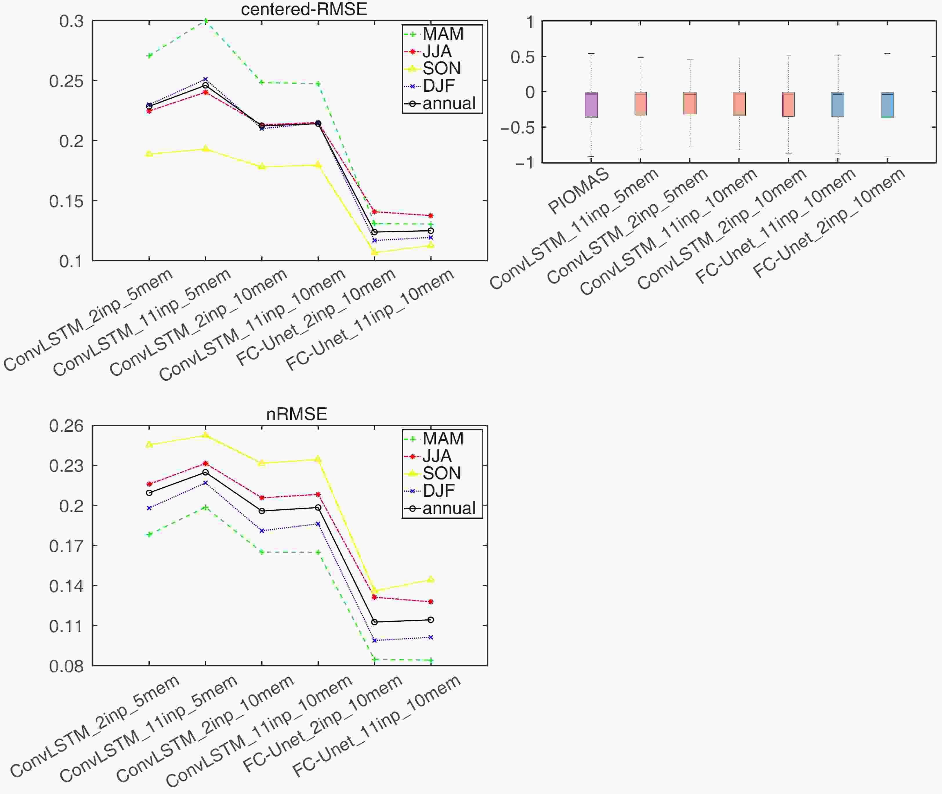
Figure 2. (left) Centered-RMSE and nRMSE between PIOMAS and predicted SIT by ConvLSTM and FC-Unet model with different data and predictor configurations. (right) The histogram of PIOMAS and predicted SITA by each experiment.
Figure 2 shows the assessments of the prediction skills of each experiment in the form of error statistics. The adopted metrics are spatiotemporally averaged centered-RMSE (standardized SIT RMSE) and nRMSE (calculated by dividing the SIT RMSE by the mean SIT of the sea ice-covered area in the corresponding month) for each season and annual period. We conduct four experiments using the ConvLSTM model (from the left of the x-axis) to assess the potential impact of data selection since the ConvLSTM model appears to be more sensitive to data quality compared to the FC-Unet (demonstrated in the next chapter). The results show that both models capture the main variability in pan-Arctic SIT relatively well, with the centered-RMSE being lowest in SON and slightly higher in MAM, which is consistent with our weighting of September samples by a factor of 1.2. Meanwhile, using more CMIP6 data for transfer learning (“10mem”) tends to result in smaller centered-RMSEs for SIT predictions, even if the additional IPSL-CM6A-LR data may introduce systematic errors at specific locations.
Meanwhile, we also assess the sensitivity of prediction skills to the introduction of additional atmospheric and oceanic variables as predictors. The predictor configurations for the experiments are also categorized into two types: one relies on the spatiotemporal fields of two sea ice variables, SIC and SIT, as indicated by the suffix “2inp” in Fig. 2. The other (denoted by the “11inp” suffix in Fig. 2) synthesize insights from several SIC forecasting studies (Fritzner et al., 2020; Kim et al., 2020; Andersson et al., 2021), which incorporate the spatiotemporal fields for the 11 climate variables listed in Table 2.
Variable Source Abbreviation or Calculation Variable name in CMIP6 Units Sea ice thickness PIOMAS SIT sithick m Sea ice concentration NSIDC SIC siconca % 10-m wind speed ERA5 sqrt(u102+v102) sqrt(uas2+vas2) m s–1 Specific humidity ERA5 q huss kg kg–1 2-m air temperature ERA5 t2m tas K Sea surface temperature ERA5 sst tos K Rain rate ERA5 mtpr-msr pr-prsn mm d–1 Snow rate ERA5 msr prsn mm d–1 Surface pressure ERA5 sp ps Pa Mean surface downward shortwave radiation flux ERA5 msdwswrf rsds W m–2 Mean surface downward longwave radiation flux ERA5 msdwlwrf rlds W m–2 Table 2. Selected predictors for DL models.
Based on the same metrics, the four x-labels with suffix “10mem” in Fig. 2 indicate that when considering the total SIT variability, to include the seasonal cycle, the introduction of more predictors seems to be harmful to prediction skills. However, noting that in climatological research, more attention tends to be paid to the anomalies relative to historical climatology. We thus evaluate the anomalies of predicted and actual SIT relative to the 1989–2015 monthly climatology (not shown). The result shows that the incorporation of a larger set of climate variables (listed in Table 2) as predictors contributes to reducing the centered-RMSEs of SIT anomalies. In addition, intermodel comparisons show that the FC-Unet model has a smaller prediction error compared to ConvLSTM. Consequently, we select the experiments with more transfer learning data and more predictors as the optimal configuration for subsequent analysis.
Moreover, the parameters for subsequent fine-tuning phases are set as follows. The fine-tuning data are split into a training set for the years 1979–2011 and a test set for 2012–20 respectively, and 10% of the training set is further split for validation. Early stopping is implemented to prevent overfitting and is only triggered if the loss on the validation set does not decrease for 10 consecutive epochs. Meanwhile, the learning rate is initialized to half the level of the transfer training phase and follows an exponentially decaying schedule. In practice, the early stopping is usually triggered within 30 fine-tuning epochs.
-
Based on ConvLSTM and FC-Unet models with optimal configurations in the previous chapter, we conduct a comprehensive evaluation of their prediction skills for Arctic SIT and SIT anomaly (SITA). Figure 3 shows the spatial correlation between predicted and actual SIT by month. The overlap of test periods for both models (2014–17) is depicted, except for 2012–13 which is reserved for subsequent extreme event assessment. Both models reproduce the spatial pattern of SIT well, with spatial correlation coefficients above the 0.95 level in most months. Meanwhile, the SIT time series can be decomposed into a superposition of a historical monthly climatology and SITA, the latter being important in climatological research but has yet to be emphasized in most previous work on deep learning prediction of Arctic SIC. We therefore calculate SITAs with the same approach as the previous section (not shown) and find that the skill differences become more significant. The correlations of FC-Unet remain consistent around the 90% level for all months, while the performance of ConvLSTM shows stronger seasonality with higher correlation during the melting season (Highest in September at ~70%, consistent with sample weight settings mentioned previously) and lower by about 10%–20% during the freezing season.

Figure 3. Mean spatial correlation between PIOMAS and predicted SIT by ConvLSTM (blue line) and FC-Unet (red line) within the time period of the test set.
In summary, the performance differences in terms of spatial correlation between the models are evident. The spatial consistency of the FC-Unet predictions with PIOMAS is reliable throughout the testing period, whereas the ConvLSTM model slightly underperforms, with stronger seasonality partly because the model is more sensitive to sample weight settings.
In addition, we also access some non-transfer learning models adopted in previous studies (Chi and Kim, 2017; Kim et al., 2020), such as the conventional CNN model trained on local samples (not shown). To overcome data scarcity, the model subdivides the pan-Arctic prediction mission into numerous local prediction tasks, each of which predicts SIT at the central grid point of an 11 × 11 local predictor (radius of ~125 km). Assessment results show that its performance significantly declines when anomalies are examined.
The deficient skill of a conventional CNN model is mainly attributed to several underlying factors. First, the feasibility assumption of this approach is that the SIT at grid points throughout the pan-Arctic region can be related to local climate variables via the same nonlinear relationship. Thus, it sacrifices larger-scale spatial information and the corresponding teleconnections. Meanwhile, the conventional CNN model simply treats different timesteps as separate features, inherently lacking the capability to extract temporal features from the inputs. As a result, there are large performance gaps compared to ConvLSTM and FC-Unet; therefore, we do not conduct follow-up assessments on it.
We then proceed to examine the temporal correlation between predicted and actual SITA by season and region. The temporal anomaly correlation coefficient (TACC) is chosen as the metric, which represents the correlation between predicted and actual anomalies. Figures 4a and 4b depict the spatial distribution patterns of TACCs for the ConvLSTM and FC-Unet models as a function of seasons. Overall, both DL models well capture the anomalous variability of SIT across the seasons, with TACC levels close to 1 over much of the pan-Arctic region. Meanwhile, the TACCs are relatively low along the eastern coast of Greenland throughout the year, and at the southern entrance to the Bering Strait during the freezing season (DJFMAM). In contrast, the TACCs drop below zero along the ice edges in the Baffin Bay and Labrador Sea, as well as in the northern part of the Hudson Bay in SON. Figure 4c depicts the differences between the two models. Relative to FC-Unet, the ConvLSTM model has lower correlations throughout the year, mainly near the North Pole and also in coastal areas with more complex land-sea distributions, such as the Canadian Archipelago, Hudson Bay, Baffin Bay, and Davis Strait. In addition, lower TACCs are also observed along the western coast of the Labrador Sea and the northern parts of the Bering and Okhotsk Seas during the freezing season.

Figure 4. Prediction skills of the (a) ConvLSTM and (b) FC-Unet models as measured by TACC for each season and annual period. (c) TACC difference between the ConvLSTM and FC-Unet model. The numbers in the upper-left corner of the subplots are the mean pan-Arctic spatial correlation coefficients.
It is worth mentioning that both two DL models have slightly lower correlations for locations near 70°E along the 110°W meridian. This is due to the setup of the grid points in the ocean module of IPSL-CM6A-LR, which creates a certain default value problem in this elongated area. Although the difference in these correlations is not very significant, to some extent it supports the finding that the ConvLSTM appears to be more sensitive to data configuration, when IPSL-CM6A-LR members are introduced as samples for training.
In summary, the TACC and MAE (Figs. 4 and 5) results are consistent; both indicate that the performance gap between the ConvLSTM and FC-Unet is mainly around the North Pole, as well as in regions with complex land-sea distribution. In these regions, subtle differences in the models’ capabilities to capture spatiotemporal features come to the forefront, thus leading to the correlation gap described above.

Figure 5. Same as in Fig. 4, but for MAE patterns. The numbers in the upper-left corner of the subplots are pan-Arctic average MAE levels.
Building upon the above results, we further conduct a systematic statistical analysis of the SITA predictions for each region using a Taylor diagram (Fig. 6). For sea area zoning, the regional mask provided by NSIDC is adopted.

Figure 6. The Taylor diagram of PIOMAS and predicted SITAs for each region.
For both models, the primary discrepancies between predictions and actual values are mainly found in the Central Arctic Ocean, Hudson Bay, and Canadian Archipelago, while the consistency is higher in other regions (Fig. 6). Overall, the SITA predictions by FC-Unet are generally consistent with PIOMAS. In contrast, as evidenced by lower correlations and larger RMSDs, the ConvLSTM model underperforms mainly in the Canadian Archipelago and Hudson Bay regions with complex land-sea distributions, as well as a slight underestimation of the magnitude of the SITA in the Central Arctic Ocean region.
Statistical analysis of the distributions of SIT predictions and true values (not shown) reveal that our conclusions are consistent with the above findings. Further, the results of statistics by season show that errors in the Hudson Bay and Canadian Archipelago regions exhibit distinct seasonality. In Hudson Bay, the discrepancies mainly appear in DJF and manifest as negative anomalies, which are more significant in the ConvLSTM model. As for the Canadian Archipelago region, the seasonality of the discrepancies is even stronger. During the freezing season, the ConvLSTM model appears to overestimate the negative SITA, whereas in summertime, both models tend to underestimate the strong negative SITA. Meanwhile, discrepancies in the Central Arctic Ocean region show a slight underestimation of the negative SITA across all seasons, with a slightly larger deviation for the ConvLSTM model.
In summary, the SITA predictions of FC-Unet are generally consistent with PIOMAS, while performance gaps for the ConvLSTM model are mainly found in regions with complex land-sea distributions, and also in the central Arctic Ocean.
We further attempt to explain the reasons for these performance gaps. The skill discrepancies in coastal regions are probably due to filling value settings. To be specific, the distribution peak of SIT is biased towards the minimal end (zero, same as the inactivated state of neurons); meanwhile, the landmask and other missing values in the samples are also filled with zeros. This results in the inability of the models to effectively distinguish between ice-free sea surface and filling values. Moreover, a higher prevalence of inactivated values can exacerbate the gradient vanishing problem. The FC-Unet model mitigates this problem to some extent by adopting the ResNet architecture (He et al., 2016) in its main composition modules, and thus outperforms the sequential ConvLSTM model. In contrast to the SIT distribution, the peak of the SIC distribution is located near its maximum value (~1). This implies that the models encounter fewer aforementioned problems when predicting SIC, which is consistent with our finding that the models’ prediction skills for SIT are slightly lower than those for SIC (not shown).
-
In September 2012, Arctic sea ice extent reached a record low of 3.63 million km2, followed by a rapid recovery to 5.35 million km2 in September 2013 (Liu and Key, 2014). Previous research suggests that anthropogenic influences played a significant role in the extreme sea ice minimum in 2012 (Kirchmeier-Young et al., 2017) and its subsequent recovery, through a combination of multiple factors. Considering the important role of Arctic sea ice in the global climate system, accurate predictions of such extreme events are essential for investigating the attribution and impacts of climate change or specific operations such as real-time shipping route planning.
Figure 7a illustrates the magnitude of the extreme sea ice minimum in September 2012, and Figs. 7b and 7c depict the difference between actual and predicted SIT/SIE by the DL models. Overall, both the FC-Unet and ConvLSTM models accurately predict the lowest historical SIE. In contrast, in the ice edge region between 120°W–180°, the prediction errors of FC-Unet are relatively small, while the ConvLSTM exhibits clear positive errors.

Figure 7. (a, d) The actual SITA, and error between the predicted and actual SITAs for (b,e) ConvLSTM and (c, f) FC-Unet for September (a–c) 2012 and (d–f) 2013, with SIE contours superimposed on each subplot (the actual SIE in green and the predicted SIE in yellow).
Similarly, the bottom row of Fig. 7 illustrates the rapid recovery of sea ice in September 2013 and its prediction errors. Figure 7d shows that the overall sea ice anomalies remained negative in the context of the multidecadal declining trend of Arctic sea ice, and both DL models exhibit similar patterns of prediction errors in Figs. 7e and 7f. In comparison, the ConvLSTM model shows a broader spread of positive errors from 120°W–60°E, and significantly larger positive errors to the north of Greenland.
In summary, both DL models are capable of predicting extreme events. This is possibly due to the incorporation of multiple climate variables as predictors, which allows the models to recognize the precursors leading to such extreme events, thus allowing for the successful prediction of abrupt changes in Arctic sea ice.
-
In this study, we build two data-driven DL models for pan-Arctic SIT monthly predictions by independently designing or modifying existing models with ConvLSTM and FC-Unet algorithms as their cores. By utilizing CMIP6 historical simulation data for transfer learning and fine-tuning with monthly observation and reanalysis datasets from 1979 to 2011, we achieve monthly predictions for pan-Arctic SIT (and SIC) from 2012 to 2017.
We first examine the sensitivity of prediction skills to the transfer-training data and predictor configurations through a set of experiments. Our findings suggest that using a broader set of CMIP6 data for transfer learning, as well as incorporating multiple atmospheric and oceanic variables as predictors, contributes to the improvement of prediction skills of both models, which mainly manifests as reductions in the centered-RMSE between the predicted and actual values.
Subsequently, we evaluate the prediction skills under the optimal configuration by season and region. Both DL models capture the overall variabilities of pan-Arctic SIT relatively well. Meanwhile, when considering the SIT anomaly independently, the FC-Unet predictions exhibit a higher and more robust consistency with actual values, with spatial correlations around the ~0.9 level for all months (mean 0.89). In contrast, the prediction skill of ConvLSTM shows more pronounced seasonality, being higher in SON and slightly lower during the freezing season. Furthermore, the performance discrepancies in MAE and temporal ACC between the two models are mainly found around the North Pole and in coastal regions characterized by a complex land-sea distribution.
In addition, we also examine the performances of both models in predicting the extremely low Arctic SIE event in September 2012 and the subsequent rapid recovery in September 2013. Both the ConvLSTM and FC-Unet reproduce the extreme SIE and SITA quite well, further strengthening our confidence in the prediction skills of both models.
Future work will focus on some specific improvements that can be made based on the results summarized above. The first step is to examine whether metadata such as landmask can be used as predictors to improve the prediction skills of the models. Meanwhile, we need to strengthen the quality control of CMIP6 transfer training data in the preprocessing stage. Moreover, further optimizations to model structure, such as applying the encoder-decoder architecture to the ConvLSTM model and refining the input block of the FC-Unet model, are also in our future work plan.
On the other hand, there are many deep learning algorithms other than those employed in this paper whose performances are worth verifying. A typical example is the Vision Transformer (Vaswani et al., 2017; Dosovitskiy et al., 2020), variants of which have been successfully applied in climatological studies such as ENSO forecasts (Gao et al., 2022). As larger numbers of reliable forecasting models become available in the future, the potential of synthesizing predictions to average out model-specific errors (Massonnet et al., 2023) deserves further investigation.
Furthermore, we would like to explore the potential of deep learning for predicting Antarctic sea ice (Wang et al., 2023). Many existing studies have shown that complex ocean-atmosphere-cryosphere processes can lead to large biases between numerical model simulations and observations of Antarctic sea ice (Purich et al., 2016; Bracegirdle et al., 2018; Hyder et al., 2018; Beadling et al., 2020). Even in the latest CMIP6 simulations, improvements in Antarctic sea ice simulations are limited relative to the Arctic (Meredith et al., 2019; Shu et al., 2020; Casagrande et al., 2023). These findings have prompted considerable interest as to whether deep learning models can correctly capture the climate features affecting Antarctic sea ice for accurate prediction.
In conclusion, our research underlines the validity and reliability of the ConvLSTM and FC-Unet algorithms in predicting Arctic SIT. The insights gained from our study can pave the way for more accurate pan-Arctic predictions, and provide significant value for climatological research and real-time business applications.
Acknowledgements. The authors thank the editor and the two reviewers for their valuable comments, which largely improved the quality of this paper. The authors of this paper were supported by the National Natural Science Foundation of China (Grant Nos. 41976193 and 42176243).
| Model | Country (Institution) | Sea ice model (resolution) | Members selected |
| ACCESS-ESM1-5 | Australia (CSIRO) | CICE4.1 (360 × 300) | historical run (r1i1p1f1 to r5i1p1f1) |
| IPSL-CM6A-LR | France (IPSL) | NEMO-LIM3 (362 × 332) | historical run (r1i1p1f1 to r5i1p1f2) |


 AAS Website
 AAS WeChat