


 DownLoad:


-
Fires, like other natural hazards such as extreme precipitation, have a substantial impact on both ecosystems and human communities, inflicting significant harm to the environment and our overall health and wellbeing. Under global warming, wildfire activities become more and more frequent globally (Jolly et al., 2015). In the western United States (WUS), wildfires have been increasing in size, frequency and severity over the last several decades (Dennison et al., 2014; Mueller et al., 2020). Previous studies have demonstrated that fire activities can significantly affect weather and climate by releasing substantial amounts of heat, gases, and aerosol particles into the atmosphere (Abatzoglou and Kolden, 2013; Liu et al., 2017; Lee et al., 2018; Zhang et al., 2019, 2022). The heat emitted from fires can increase low-level temperatures and dramatically impact environmental thermodynamics (Trentmann et al., 2006; Kablick III et al., 2018; Zhang et al., 2019); fire-induced aerosols can impact severe convective storms (SCSs) and climate through aerosol–radiation and aerosol–cloud interactions (Lindsey and Fromm, 2008; Lu and Sokolik, 2013; Logan et al., 2018; Zhang et al., 2019, 2022).
However, studies of the impacts of fire on SCSs have tended to focus on either pyrocumulonimbus clouds (Fromm et al., 2006; Cunningham and Reeder, 2009; Kablick III et al., 2018; Zhang et al., 2019) or the local impact of wildfire aerosols (Lindsey and Fromm, 2008; Grell et al., 2011; Lu and Sokolik, 2013; Lee and Wang, 2020). The remote impact of fires on SCSs has not yet been explored to a sufficient extent. For example, large WUS wildfires emit enormous quantities of aerosols and sensible heat during the wildfire season, which could impact the environment for severe weather in the central United States (CUS). However, WUS wildfires occur most often in late summer and fall, which do not coincide with the severe weather seasons (i.e., spring and summer) in the CUS. Nonetheless, it has been observed that wildfires in WUS have begun to start earlier and earlier under climate change (Westerling et al., 2006; Jain et al., 2017; Jacobo and Zee, 2021). For example, the fire season in 2018 started in May in both the WUS and CUS. Such an earlier start to the fire season extends its duration and leads to it more likely coinciding with the severe weather season in the CUS. During the week of 23–29 July 2018, there was an extreme co-occurring event with storms occurring on four to five consecutive days and large western wildfires (e.g., Carr Fire and Mendocino Complex Fire).
In an earlier study, we simulated this extreme case with detailed physics and explored the remote effects of western wildfires on precipitation and hail in the CUS (Zhang et al., 2022—hereafter referred to as Zhang2022). Model results showed that WUS wildfires notably increase the frequencies of heavy precipitation rate (> 40 mm h−1) and significant severe hail (> 5.08 cm) in the CUS, through the effects of both aerosol and sensible heat from wildfires. The model results revealed a synoptic-scale change in weather caused by WUS wildfires; that is, enhanced westerly winds, which make the meteorological environment more conducive to SCSs and increase the transportation of aerosols. However, this modeling study based on cases had limitations in terms of generality, particularly considering the stochastic nature of convective storm simulations.
Following on Zhang2022, here, we systematically examine the impacts of WUS fires on CUS SCSs over a two-decade period from 2001 to 2020 using machine learning (ML) methods. Zhang2022 showed that co-occurring cases of western wildfires and central SCSs are limited during a 10-year period. Therefore, to increase the sample size for reliable ML analysis, we not only extend the study period to 20 years, but also consider all fire types, including prescribed and agricultural fires, in selecting the co-occurring events. ML models are built to explore the linkage between hailstones in the CUS and the features of WUS fires (e.g., fire size, fire intensity, and smoke aerosols), with consideration of both meteorological factors and smoke aerosols over the fire regions as well as along the transport path. Two tree-based ML models that use ensemble learning algorithms—namely, Random Forest (RF) (Breiman, 2001) and Extreme Gradient Boosting (XGB) (Chen and Guestrin, 2016)—are adopted and developed to extract the nonlinear relationships between WUS fires and CUS hailstorms and examine variable contributions for the prediction of hailstones. To gain robust feature rankings for the constructed ML models, we use Shapley additive explanation (SHAP) values (Nohara et al., 2019) from both the RF and XGB models to evaluate the contribution of each predictor.
The ensemble learning approaches in RF and XGB can address the limitations of traditional linear regression methods in representing complex nonlinear relationships with variable interactions and obtain a robust predictive understanding of the occurrence of hail in the CUS associated with WUS fires. The findings can provide insights for designing long-term infrastructure or mitigating risk associated with these extreme events.
The rest of paper is structured as follows: We first introduce the data and ML methodology in section 2. Section 3 presents the development and evaluation of the two ML classification models for the occurrence of large hail in different regions and states and discusses the contributions of the most important variables influencing the occurrence of large hail. We summarize the limitations and applicability of the ML model and future work in section 4.
-
The fires in the WUS considered in this study are from California (CA), Oregon (OR) and Washington (WA), while the hail in the CUS is from Montana (MT), Wyoming (WY), Colorado (CO), New Mexico (NM), North Dakota (ND), South Dakota (SD), Nebraska (NE), Kansas (KS), Oklahoma (OK), and Texas (TX), as shown in Fig. 1. MT, WY, CO, and NM are near the Rocky Mountains and are referred to as the original column 1 states (original CS1), while ND, SD, NE, KS, OK and TX are further downstream and are referred to as the original column 2 states (original CS2) (Fig. 1).

Figure 1. Map of fire states in the WUS and hail states in the CUS. The three fire states in the WUS (highlighted by red points) are WA, OR and CA. The CUS states are divided into two columns: the original CS1 (i.e., MT, WY, CO, and NM) and original CS2 (i.e., NE, SD, NE, KS, OK and TX). States scattered with blue points are those more likely to be affected by fires in the WUS. The green dashed rectangle denotes the region with westerly winds in general, which is considered as the plume transport path from the WUS to the CUS.
The study period is from 2001 to 2020. Only the warm season from March to September is considered since hailstorms are minimal in the cold season. The data selection process for co-occurrences of WUS fires and CUS hail is detailed in section 2.1.1. The two tree-based ML models (i.e., RF and XGB) are developed to understand the relationships between the daily hail occurrence for large hail with hail size ≥ 2.54 cm in the CUS and the fire features in the WUS (e.g., fire size, fire intensity, and smoke aerosols), with consideration of the co-located meteorological variables (e.g., air temperature, U-wind) over fire regions and along the path of fire plumes. The trained ML models are used to identify the important fire features and co-located meteorological variables contributing to the hail characteristics for physical understanding. Section 2.1 introduces the data used in this study, and section 2.2 describes the methodology of the tree-based ML models, the model performance evaluation metrics, and variable ranking.
-
The hail observational datasets used for this study are from the National Oceanic and Atmospheric Administration’s Storm Prediction Center (SPC) database. The advantage of using hail reports from SPC is the confidence in the occurrence of hailstones on the ground. However, hail reports could underestimate the hail size—for example, due to surface melting prior to and during hail size measurement (Blair et al., 2011, 2017). This underestimation in hailstone size is more obvious for smaller hail sizes, as they tend to melt faster. Smaller-sized hailstones are less likely to cause direct damage compared to large hail (size ≥ 2.54 cm). Therefore, in this study, we mainly focus on large hail with size ≥ 2.54 cm, which covers both severe hail (2.54–5.08 cm) and significantly severe hail (≥ 5.08 cm). For each state over the study region of the CUS, we calculate the large hail occurrence and the large hail count from March to September (warm season) over the period of 2001–20 (Table 1). The daily large hail occurrence in a specific state is considered with a threshold, i.e., 1 means that the daily total number of large hail count is greater than a threshold, and 0 otherwise. This is to exclude very minor hail events, which would not produce much impact and are difficult to predict. To check if the choice of a specific threshold for the total number of hail counts will affect the prediction of large hail occurrence in a specific state, two hail count thresholds (i.e., 10 and 20) are considered. These labeled hail occurrences are then used as the target variables in the ML classification models.
Target variables Abbreviation Temporal resolution Data Source Daily occurrence of hail with size ≥ 2.54 cm (0/1) in a state Hail occurrence daily SPC Daily hail count for hail with size ≥ 2.54 cm in a state Hail count daily SPC Predictor variables Abbreviation Temporal resolution Data Source Mean maxFRP for fire grids in three WUS states within t days before hail maxFRP _m_COW_dt daily MODIS Maximum maxFRP for fire grids in three WUS states within t days before hail maxFRP_max_COW_dt daily MODIS Mean maxFRP for fire grids in states within t days before hail maxFRP_m_s_dt daily MODIS Maximum maxFRP for fire grids in states within t days before hail maxFRP_max_s_dt daily MODIS Total number of fire grids in three WUS states within t days before hail ngrids_COW_dt daily MODIS Total number of fire grids in states within t days before hail ngrids_s_dt daily MODIS Temporal change of fire grids in three WUS states within t days before hail gdiff_COW_dt daily MODIS Temporal change of fire grids in states within t days before hail gdiff_s_dt daily MODIS Mean BC+OC over fire grids in three WUS states within t days before hail BCOC_m_COW_dt daily MERRA-2 Maximum BC+OC for all grids in three WUS states within t days before hail BCOC_max_COW_dt daily MERRA-2 Mean BC+OC over fire grids in states within t days before hail BCOC_m_s_dt daily MERRA-2 Maximum BC+OC for all grids in states within t days before hail BCOC_max_s_dt daily MERRA-2 Mean RH at 850 hPa over three WUS states within t days before hail RH850_m _dt daily MERRA-2 Maximum RH at 850 hPa over three WUS states within t days before hail RH850_max _dt daily MERRA-2 Mean air temperature at 850 hPa over three WUS states within t days before hail T_m _dt daily MERRA-2 Maximum air temperature at 850 hPa over three WUS states within t days before hail T_max _dt daily MERRA-2 Mean U-wind at 850 hPa for grids along fire path within t days before hail U850_m_dt daily MERRA-2 Maximum U-wind at 850 hPa for grids along fire path within t days before hail U850_max_dt daily MERRA-2 Mean U-wind at 250 hPa for grids along fire path within t days before hail U250_m_dt daily MERRA-2 Maximum U-wind at 250 hPa for grids along fire path within t days before hail U250_max_dt daily MERRA-2 Notes: t ∈[1,2] for U-wind; t ∈[2,4] for other variables; s∈[CA, OR, WA]; the fire transport region (38°–44°N, 125°–112°W) Table 1. Target and predictor variables used in the ML models.
As mentioned in the Introduction, this study follows on from the modeling study of the impacts of WUS wildfires on weather hazards in the CUS in Zhang2022. Different from Zhang2022 in which wildfire data from the Fire Program Analysis Fire-Occurrence Database (FPA-FOD) were used, here, we use the thermal anomaly datasets from the Terra Moderate Resolution Imaging Spectroradiometer (MODIS) Thermal Anomalies and Fire Daily (MOD14A1) Version 6. Unlike FPA-FOD, which only includes wildfires reported from federal, state, tribal, and local governments, MOD14A1 has fire-related thermal anomaly detection, capturing all types of fires, including wildfires, agricultural field burning, prescribed fires, etc. (Huang et al., 2012; Wang and Wang, 2020). The datasets are generated at ~1 km spatial resolution and daily temporal resolution. The variables include the fire mask, pixel quality indicators, maximum fire radiative power (maxFRP), and the position of the fire pixel within the scan. Individual 1-km pixels are assigned to one of nine fire mask pixel classes, which indicate the different confidence levels of fire occurrence. In this study, we only use the fire pixels with the highest confidence level to calculate the daily fire features for individual fire states (i.e., CA, OR, or WA) as well as the whole WUS region (i.e., CA + OR + WA). The fire features include the mean and maximum maxFRP, total number of fire pixels, and the temporal change of fire pixels (the change in the daily total number of fire pixels compared with that of the previous day) for each fire day (Table 1). The black carbon and organic carbon aerosols (BC+OC), characteristic of smoke aerosols in the fire regions, are also considered. We use the column-integrated mass concentrations of BC+OC from the Modern-Era Retrospective Analysis for Research and Applications, Version 2 (MERRA-2) (Gelaro et al., 2017) to represent the smoke aerosols over WUS fire regions. Here, we only consider fires with daily burned areas no smaller than 20 km2 (i.e., the top 30% of daily burned areas of WUS fires). Small fires with total burned areas less than 20 km2 over the WUS are not considered in this study, as their impacts on remote hailstorms should be minor or even negligible, especially when the fire pixels are sparsely distributed over the WUS.
Besides identifying co-occurring events of WUS fires and CUS hailstorms, the WUS fires (≥ 20 km2 in size) need to co-occur with hailstorm days (daily hail counts ≥ 10 or 20 over the CUS). To account for the time lag for the remote effect of WUS fires, we also require fires to exist within 2–4 days before the occurrence of hailstorms, based on the estimate of aerosol optical depth changes in Zhang2022. For example, for a selected storm occurring on 26 July, not only that day but also 24 and 25 July must be fire days for the 2-day requirement (we tested 3 and 4 days to judge the sensitivity). The co-occurring events identified with daily hail counts ≥ 20 over the CUS in each year are shown in Fig. 2. As discussed earlier, use of MODIS fire data, which include all kinds of fires, increases the sample size of co-occurring events compared with Zhang2022 in which only wildfires were considered. We have about 30 co-occurring events in 2008 and 2009, and more than 25 events in 2013, 2015 and 2016. There is no significant trend in the time series (Fig. 2).

Figure 2. Time series of co-occurring events of WUS fires and CUS large hail identified with daily hail counts ≥ 20 and fire size ≥ 20 km2.
-
Other than WUS fire features (e.g., fire size, fire intensity, and smoke aerosols), the meteorological variables over the fire region and along the paths of fire plumes are considered in this study based on physical mechanisms revealed in Zhang2022. These meteorological variables include air temperature (T), relative humidity (RH), and U-wind. Behaviors of individual fires are determined by fire weather characterized by atmospheric elements such as T, RH, wind etc. (Liu et al., 2013). As with the smoke aerosols (BC+OC), the meteorological variables are also obtained from MERRA-2 to be physically consistent. The MERRA-2 data for BC+OC, T, RH, and U-wind are available every three hours at an approximate spatial resolution of 0.5° × 0.625° and 72 hybrid-eta levels. Here, we use the values at 850 hPa for BC+OC, RH and T, and values at 250 hPa and 850 hPa for U-wind. The daily mean and maximum values for BC+OC, RH, and T are summarized over individual states (i.e., CA, OR, or WA) as well as the whole WUS region (i.e., CA + OR + WA) within 2–4 days before each hail day. Here, a hail day is defined as a day with total hail counts of at least 10 or 20 over the CUS. For U-wind, the daily mean and maximum values are calculated approximately along the paths of fire plumes [green dashed rectangle (38°–44°N, 125°–112°W) in Fig. 1] within 1–2 days before each hail day. Combining all these attributes as shown in Table 1, we have a total of 91 variables in the predictor matrix, which will be used as the inputs for training the ML models.
-
To study the impacts of fire features and their associated meteorological variables in the WUS on the hail characteristics in the CUS, RF and XGB models are built to model their complex and nonlinear relationships using the hail occurrence as the target variable. RF is a tree-based ensemble ML method for regression and classification, which was developed by Breiman (2001). It is mainly used to construct a prediction model in a supervised learning problem. It can also be used to evaluate the predictor variables with respect to their ability to predict the response (Boulesteix et al., 2012). XGB is an ensemble learning method based on the idea of boosting (Chen and Guestrin, 2016). The boosting approach incorporates multiple decision trees and combines all the predictions to obtain the final prediction. XGB is an implementation of gradient boosted decision trees, a weighted ensemble of weak prediction models. It is designed to prevent overfitting and to be computationally more efficient than the gradient boosting machine.
The CS1 and CS2 states (Fig. 1) have different distances from the WUS regions and the fire impacts are expected to be different. Therefore, ML models are built separately for CS1 and CS2 states. We further investigated the effects on the states located further downstream, specifically in the Midwest, and found the impact to be minimal. Consequently, our focus is primarily on the CS1 and CS2 states. The ML models for predicting hail occurrence (i.e., daily hail occurrence with hail size ≥ 2.54 cm in a specific state) in CS1 and CS2 are built by randomly selecting 80% of the dataset for training and 20% for testing. We then validated the ML models using five-fold cross-validation. Each ML model is formulated as
where
$ {f}_{\mathrm{c}\mathrm{l}\mathrm{a}\mathrm{s}\mathrm{s}\mathrm{i}\mathrm{f}\mathrm{i}\mathrm{e}\mathrm{r}}(.) $ is an RF or XGB classifier, built to predict the probability of hail occurrence ($ {y}_{p} $ ) in the CS1 states and CS2 states, and x1, x2… xi are the predictor variables, as shown in Table 1.Various evaluation metrics are used to evaluate the model performances. The classification models are evaluated by their accuracy, precision, recall, and F1 score. Precision and recall are defined as follows:
where “true positive” indicates the occurrence of large hail is correctly predicted by the model; “false positive” is where large hail does not occur but is predicted as an event, and “false negative” measures where the model fails to predict the occurrence of large hail when it does occur. The F1 score measures a model’s accuracy by combining the precision and recall:
The F1 score has a maximum value of 1 and a minimum value of 0, and a higher F1 indicates a higher balance between precision and recall.
In binary classifications, a model gives us a probability instead of the prediction (0/1) itself, so we need to convert this probability into a prediction by applying a classification threshold (e.g., default threshold of 0.5). However, the default threshold of 0.5 may not represent an optimal interpretation of the predicted probabilities, particularly for a classification problem with very imbalanced data. For example, in this study, the hail days over March to September from 2001 to 2020 are less than 20% of the total days in either CS1 or CS2. One way to find the optimal classification threshold is by checking and balancing the precision and recall values for the RF and XGB models and adjusting the classification thresholds ranging from 0 to 1.
As mentioned above, the set of predictor variables listed in Table 1 has a total of 91 variables. Such a high dimensionality of the predictor matrix is usually associated with issues like data collinearity. This may affect the variable rankings of the constructed RF and XGB models. To gain more robust variable rankings, we use the Shapley additive explanation (SHAP) (Nohara et al., 2019) values from both RF and XGB to evaluate the importance of a variable to the prediction of hail characteristics. SHAP is a novel approach to explain individual local and global variable importance based on game theory (Lundberg and Lee, 2017). When applying game theory to the explanation of variable importance, the predictor variables are considered as “players” in the operative game in which the goal is a prediction for a single observation. Each predictor variable obtains a “payout” based on its contribution to the game, so the “payout” is the corresponding variable importance. For a predictor variable, the SHAP value considers the difference in the model predictions made by including and excluding the predictor variable for all combinations of predictors. Variables with a larger mean absolute SHAP value (MASV) are relatively more important. This means those variables have higher predictive power and contribute more to the prediction of the target variables. In this study, we render the MASV from both RF and XGB to evaluate the variable importance by introducing the relative MASV. The relative MASV for a specific variable is calculated as
where
$ {R}_{i} $ is the relative MASV for variable$ i $ , n is the total number of predictor variables,$ {\mathrm{M}\mathrm{A}\mathrm{S}\mathrm{V}}_{i}^{\mathrm{R}\mathrm{F}} $ is the MASV for variable$ i $ from the RF model, and$ {\mathrm{M}\mathrm{A}\mathrm{S}\mathrm{V}}_{i}^{\mathrm{X}\mathrm{G}\mathrm{B}} $ is the MASV for variable i from the XGB model. Based on the relative MASV, variables that are in the top rankings are identified as important predictors for states in CS1 and CS2. -
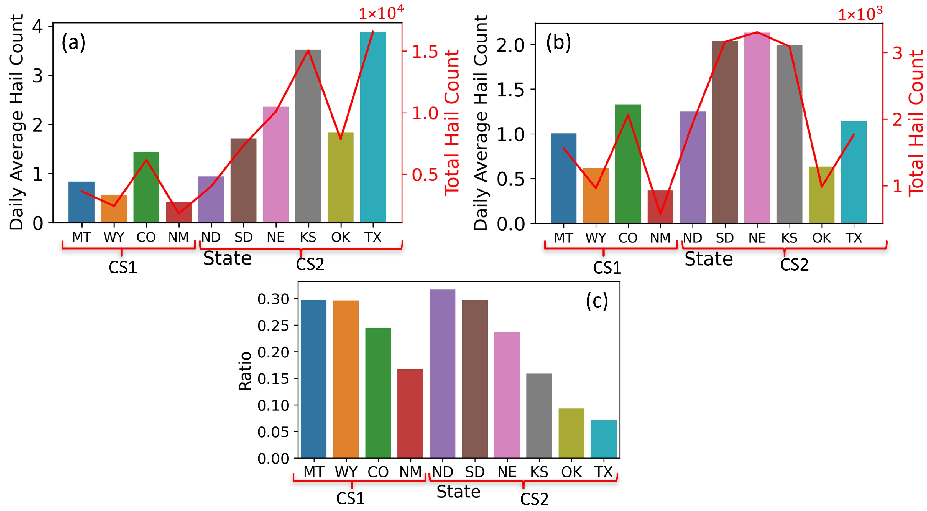
We first examine the daily average large hail count and total large hail count from March to September over the period of 2001–20 for each CUS state without considering the occurrence of WUS fires (Fig. 3). Figure 3a shows that there is generally more hail occurring in the original CS2 (i.e., ND, SD, NE, KS, OK, TX), especially in KS and TX, and less hail in the original CS1 (i.e., MT, WY, CO, NM), with a minimum in NM. After considering the co-occurrence of WUS fires with a daily burned area ≥ 20 km2 (i.e., the top one-third daily fire burned areas of WUS fires) within 2–4 days before the occurrence of large hail, states such as CO, ND, SD, NE and KS have more co-occurring events. However, in NM, OK and TX, many more hail events are irrelevant to the fires in the WUS (Fig. 2b). Therefore, in the following section, we exclude NM, OK and TX from our analysis, and focus on the states with higher ratios of co-occurring events. The two original state columns are updated with redefined states. That is, CS1 includes MT, WY and CO, and CS2 includes ND, SD, NE and KS.

Figure 3. (a) Large hail count (size ≥ 2.54 cm) for each CUS state without considering fire. (b) Large hail count for each CUS state with WUS fires of which the burned area is no less than 20 km2 and occurred within 2–4 days before the occurrence of large hail. (c) Ratio of co-occurring hail counts to total hail counts for each state.
-
As mentioned in section 2, when labeling the large hail occurrence (0/1) in a specific CUS state, a hail count threshold (i.e., whether the daily total number of hail counts over the study region is greater than the threshold) is used to exclude minor hail events. We consider two thresholds (i.e., 10 and 20 daily hail occurrences) to see how sensitive the RF and XGB classification model results are to these thresholds. We find that, even though the data imbalance is worse for the threshold of 20 (i.e., about 9.2% and 13.5% of the data are labelled as 1 for CS1 and CS2, respectively), the performance of the constructed ML classification models is obviously better than when using the threshold of 10. Therefore, for the following discussion, we only focus on the results using the hail count threshold of 20.
We evaluate the performance of the constructed classification models, RF and XGB, using the average accuracy, precision, recall, and F1 score from five-fold cross-validation. By checking the precision and recall curves for the RF and XGB models using the classification threshold range from 0 to 1, we find that the optimal classification threshold is around 0.3 (Fig. 4), instead of the default threshold of 0.5. Therefore, the accuracy, precision, recall, and F1 scores (Figs. 5 and 6) in this section are obtained using a classification threshold of 0.3.

Figure 4. Precision (blue), recall (red), and F1 score (green) curves of the (a, b) RF and (c, d) XGB models for CS1 and CS2 with the classification threshold ranging from 0 to 1. The red solid line shows the optimal classification threshold.
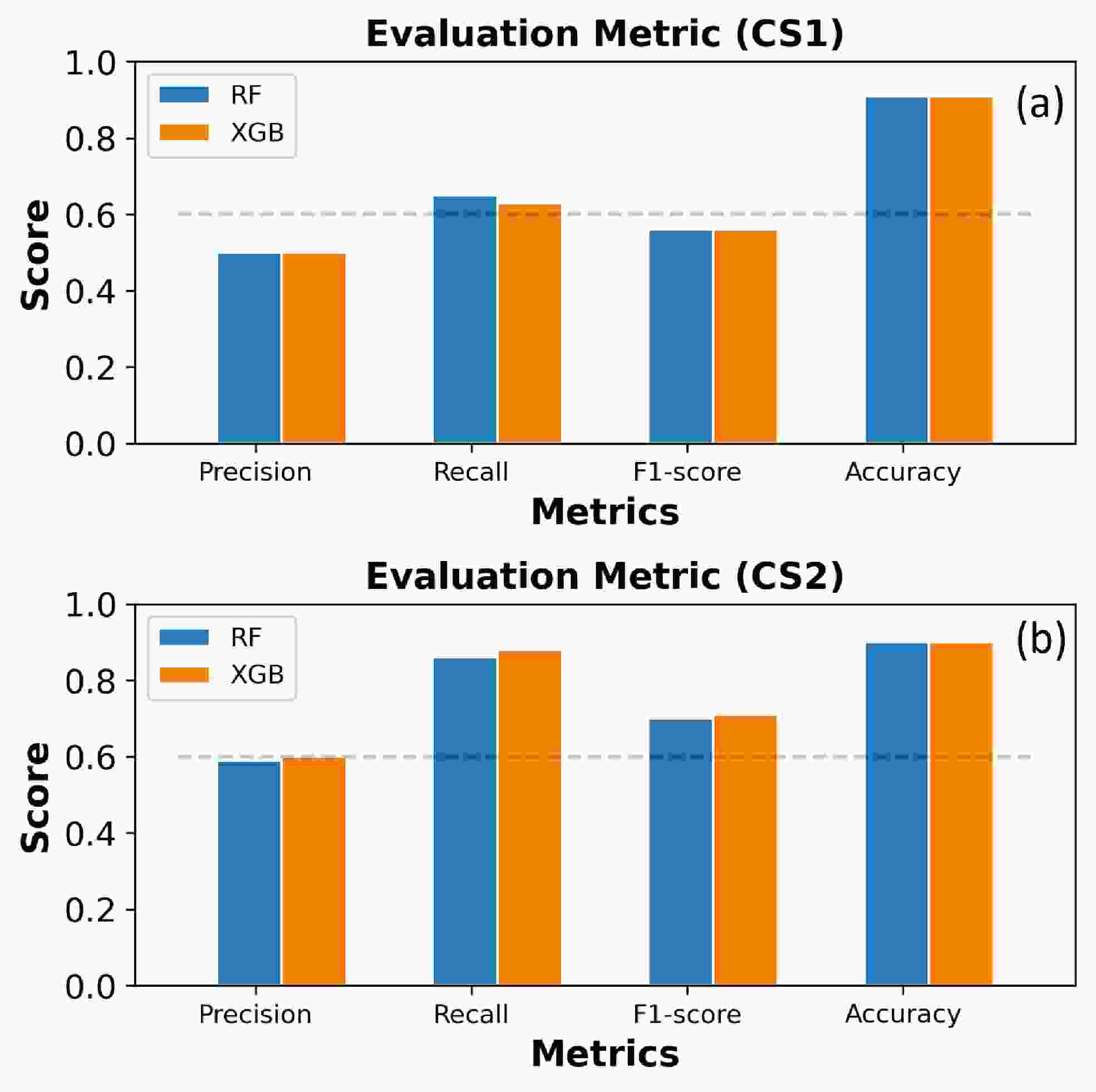
Figure 5. Average precision, recall, F1, and accuracy scores from five-fold cross-validation of the RF (blue) and XGB (orange) models for predicting large hail occurrence in (a) CS1 and (b) CS2 states.
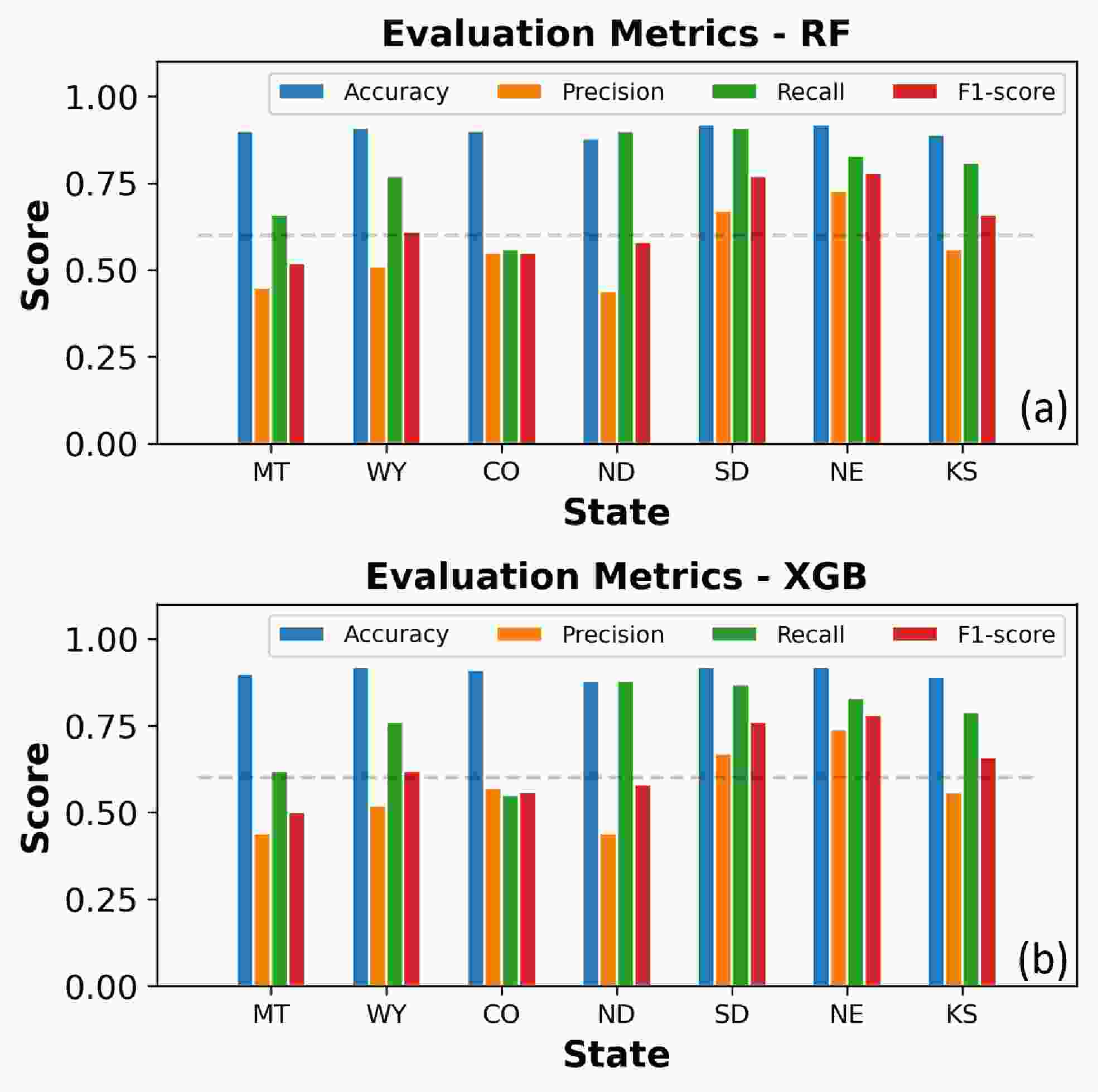
Figure 6. Average precision, recall, F1, and accuracy scores from five-fold cross-validation of the (a) RF and (b) XGB models for predicting large hail occurrence in each state in CS1 and CS2.
The overall ML classification model performances summarized from five-fold cross-validation for CS1 and CS2 are shown in Fig. 5. We can see that the values of these evaluation metrics between RF and XGB are comparable, both with a test prediction of about 90%, recall scores of 0.63–0.88, precision scores of 0.5–0.6, and F1 scores of 0.56–0.71. These results indicate that the occurrence of CUS large hail is correlated with the WUS fire features and related meteorological variables. The precision score is a bit low compared to the other metrics for both CS1 and CS2. The low precision score means that the ML model prediction returns a certain number of false positives (i.e., days without large hail occurrence are predicted as days with large hail). Interestingly, both RF and XGB perform better in CS2, with precision scores close to 0.6, recall scores up to 0.88, and F1 scores greater than 0.7, probably because of more co-occurring cases in these states, as shown in Fig. 2b.
To check if the constructed ML models can achieve good classification for each state, we also evaluate their performance in these CUS states individually, as shown in Fig. 6. Overall, the RF and XGB models are relatively better at predicting large hail occurrence in WY, SD, NE and KS, with precision ranging from 0.52–0.74, recall from 0.76–0.87, the F1 score from 0.61–0.78, and accuracy from 89%–92%. Three out of the four states mentioned above are CS2 states. This explains why the ML models for CS2 perform better than those for CS1, as shown in Fig. 5, which might be related to the many more hail occurrences in the CS2 states (Fig. 3b). Both models perform best in NE, with an accuracy of 92% and F1 score of 0.78, suggesting the impact of WUS fires may be the most significant in this state. The precision scores for MT and ND are slightly less than 0.5, relatively lower than the other five states. This suggests the correlation between WUS fires and the occurrence of large hail is not as strong as in the other states statistically. However, with the F1 score greater 0.5, the performance of ML models in these two states is still acceptable. Also, it should be noted that both MT and ND are located at the northern part of the CUS, which deviates slightly from the typical path of westerly winds.
-
The results in the previous section show that the ML models make better predictions for large hail occurrence in the CS1 state WY, and the CS2 states SD, NE and KS, than other states. For these four states with the best ML model performance, we further examine the variable importance for predicting large hail occurrence (0/1) using SHAP values. The importance of a predictor derived from SHAP is measured by calculating the relative MASV using Eq. (5) for each predictor across all available data from specific states. Variables with larger relative MASV are more important, which means those variables have higher predictive power in terms of predicting large hail occurrence (0/1).
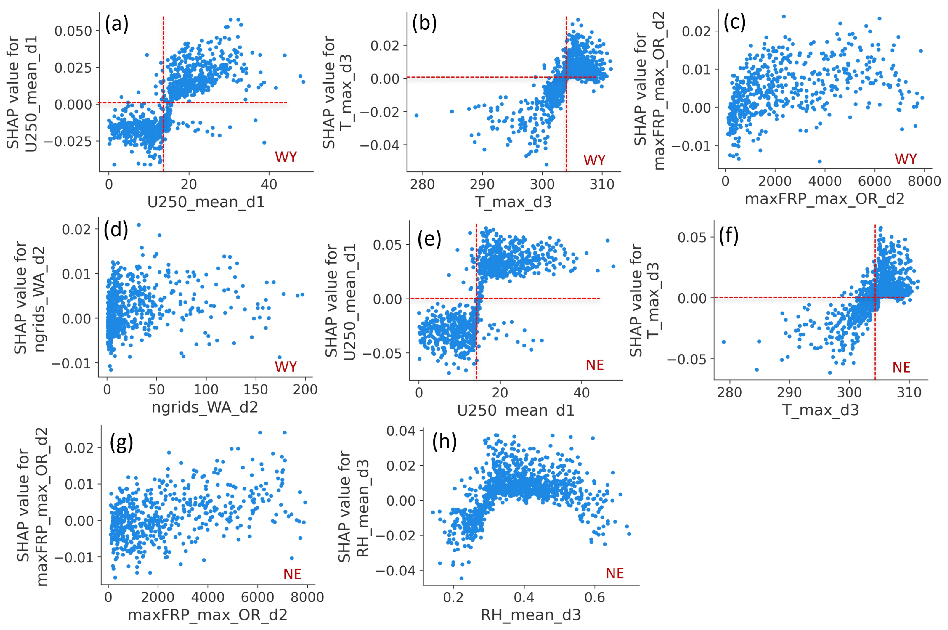
When all the states in CS1 and CS2 are concerned, the variable importance using the relative MASV show that U-wind at the high levels (250 hPa) over the path of fire plumes, the maximum air temperature (T_max), and RH related variables at the low levels (850 hPa) in the wildfire region are identified as the most important variables. As we explore the local variable importance for the four states where ML models perform the best (i.e., WY, SD, NE, and KS), we find that not only the meteorological variables mentioned above, but also the fire-related features such as maxFRP, are identified as important predictors (Fig. 7). This indicates a strong linkage between these fire attributes and hail occurrences. In SD, NE and KS, four out of the top 10 variables are maxFRP-related variables. From the patterns of the SHAP values for maxFRP (Figs. 8c, g), the SHAP values increase as the values of maxFRP increase, confirming a positive correlation between maxFRP and the large hail occurrence in these states. Compared to maxFRP, the number of fire pixels in WA (i.e., ngrids_WA_2) seems to have less impact on the large hail occurrence, as the SHAP values do not obviously correspond to the increase in the number of fire pixels (Fig. 8d). We notice that only the fire variables in OR and WA show up in the top 10 list for these four states (Fig. 7). This implies that occurrences of large hail in these four CUS states (WY, SD, NE, and KS) may be impacted more by the fires in OR and WA than those in CA.

Figure 7. Top 10 most important variables for (a) WY, (b) SD, (c) NE, and (d) KS.

Figure 8. The SHAP values for selected variables (e.g., U250, T_max at 850 hPa, maxFRP, etc.) in (a, b) WY and (c, d) NE. The SHAP values for the selected variables in SD and KS show similar patterns as those in NE.
Of all the predictor variables, the upper-level wind-related variable, the mean of U-wind at 250 hPa (e.g., U250_mean_d1), seems to be the most influential in these four states (WY, SD, NE, and KS; Fig. 7). It has a positive impact on downwind hail occurrence (Figs. 8a, e), with SHAP values greater than 0 when its mean value is greater than ~15 m s−1. The U-wind at 250 hPa within 1–2 days before hail (e.g., U250_mean_d1 and U250_mean_d2) is also among the most important variables for large hail occurrence in these four states. All these findings corroborate the mechanism proposed in Zhang2022, i.e., enhanced westerly winds increase the advection of aerosols and moisture from the wildfire region to the CUS and make storms more severe. In addition, the low-level maximum temperature in the fire region (T_max at 850 hPa) has a positive impact on the hail occurrence in WY (Fig. 8b) and NE (Fig. 8f) when its value reaches about 303 K (~30°C). Similar patterns of the SHAP values for T_max are found in SD and KS as well. The significant contributions of T_max within 2–4 days before hail (e.g., T_max_d3 and T_max_d2) suggests that the substantial amount of heat released by WUS fires may impact the atmospheric environments significantly, and affect the occurrence of CUS large hail. This is also in good agreement with Zhang2022, in which detailed modeling showed the sensible heat from wildfires plays a comparably important role as wildfire aerosols. The low-level moisture (RH at 850 hPa), such as RH850_max_d3 and RH850_mean_d3, in the WUS, is important for SD, NE and KS, because the moisture transport can intensify the storms in the CUS. This is also reflected in Fig. 8h, which shows that the SHAP values for RH850_mean_d3 in NE increase as the RH increases to a certain level (~0.4).
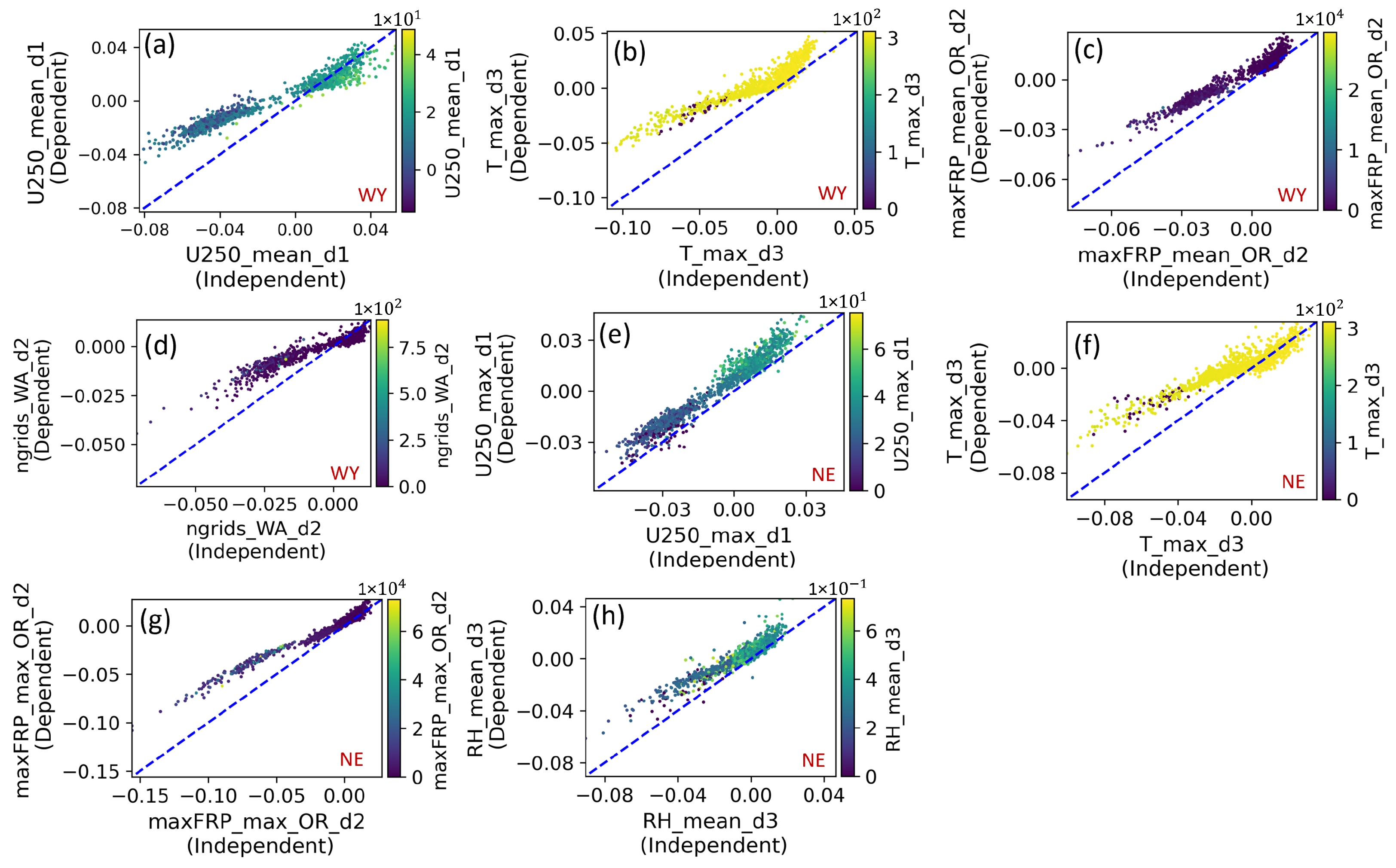
To further understand the cross-dependence among these predictors and their effects on large hail occurrence, the SHAP values for the most important variables with assumptions of independence and dependence among variables are presented in Fig. 9 for WY and NE. Independence here means there is no correlation between predictor variables; otherwise, the predictor variables are dependent. When estimating SHAP values, there are different possible assumptions about the feature dependence. When using the “dependence” approach, SHAP values are computed by introducing each predictor, one at a time, into a conditional expectation function of the model’s output (Lundberg et al., 2020). The “independence” approach breaks the dependencies between predictor variables according to the rules dictated by causal inference (Janzing et al., 2019). Therefore, if a predictor variable is dependent, we should be able to see the difference in the SHAP values between the two approaches.

Figure 9. SHAP values for the most important variables from both the RF and XGB models of (a–d) WY and (e–h) NE when assuming independence (x-axis) versus dependence (y-axis). Similar patterns for the SHAP values of these variables are found in SD and KS. The color scheme represents the values of variables.
For both WY (Figs. 9a–d) and NE (Figs. 9e–h), we see that the SHAP values for U250, T_max at 850 hPa, maxFRP, ngrids, and RH-related variables are a bit off the diagonal dashed line at the lower tail. This suggests those important variables may interact with other variables at a certain value range, and their interaction may also have some impacts on the occurrence of large hail.
Besides these important variables identified by both RF and XGB shown in Fig. 7, we also find some differences in the rankings between RF and XGB. For example, although the maxFRP in OR and WA (e.g., maxFRP_max_OR_d2 and maxFRP_max_WA_d2 in Fig. 7) are among the top 10 rankings for both the RF and XGB models, the daily maximum smoke aerosols (BC+OC) in CA and OR (e.g., BCOC_max_OR_d2 and BCOC_max_CA_d2) show up in the top 20 rankings for XGB models only. Since smoke aerosol is not shown in the top 10 rankings and the top variables identified by the ML are not independent as shown in Fig. 9, we check if there is any collinearity between them. We find that the correlation coefficients between smoke aerosols and burned area in WA and OR are 0.55–0.57 (Figs. 10a, b), and are ~0.5 between smoke aerosols and the maximum fire power (Figs. 10c, d). The SHAP independence versus dependence plots (Figs. 9c, g) show both the maximum fire power and burned area are interactive with other variables. Therefore, it is probably the data collinearity between smoke aerosols and these variables that affect their different rankings in the ML models. The contribution of smoke aerosol effects could be considered through the maximum fire power and burned area. Therefore, the effect of smoke aerosol cannot be excluded based on the ML analysis.

Figure 10. Correlation of smoke aerosols with burned area in (a) WA two days before and (b) OR three days before, and with maximum fire power in OR (c) four days and (d) three days before the large hail event.
In summary, the ML results indicate that the meteorological variables in the fire region (temperature and moisture), the westerly winds that induce the transport of aerosols and moisture from the WUS to CUS, and the fire features (i.e., maximum fire power and burned area) may contribute to the occurrence of large hail in the CUS. The results confirm a linkage between WUS fires and severe weather in the CUS, corroborating the findings of our previous modeling study with detailed physics (Zhang2022). The effects of smoke aerosol cannot be excluded due to the colinearity of smoke aerosol with fire power and burned area.
-
In this study, we employed tree-based ML methods to study the relationship between WUS fires and the occurrence of large hail in the CUS using 20 years of fire and hail data (from 2001 to 2020). To do so, ML classification models were built to predict the occurrence of large hail in the CUS states, using the co-occurring WUS fire features and the related meteorological variables over the fire region and along the path of fire plumes as predictors. The resulting RF and XGB classification models can make accurate predictions for the occurrence of large hail in some central US states with ~90% accuracy and F1 scores up to 0.78. This indicates WUS fires are correlated with the occurrence of large hail in the CUS. The ML analysis also shows that, compared to the CS1 states, WUS wildfires could have a larger impact on some CS2 states (further downwind than CS1), which may be related to more frequent hailstorms in the CS2 states. Additionally, ML models perform the best in the four states (WY, SD, NE, and KS) that are within the path of fire plumes, with large hail occurrences impacted more by the fires in OR and WA than those in CA. For MT and ND, located in the northern part of the CUS, which deviates slightly from the path of westerly winds, the performances of the ML classification models are not as good as those for the other states mentioned above, indicating the impact of WUS fires may be insignificant.
The SHAP rankings of the RF and XGB models identify the low-level temperature and RH in the fire region and westerly winds, which are related to the transport of moisture and aerosols, as the most important variables for the prediction of large hail occurrence in CS1 and CS2. For the four states where the ML models perform the best, fire features such as maximum fire power and burned area, are identified as important variables by both RF and XGB. Smoke aerosol is also identified by XGB as a top-20 important variable. Although smoke aerosol is not shown among the top 10 most important variables in ML models, it is correlated with fire power and burned area, and thus its contribution might be taken into account through these variables in the ML models. In short, the ML analysis of these 20 years of data show a relationship between WUS fires and the occurrence of CUS large hail, which corroborates the modeling study of Zhang2022. Based on Zhang2022 and this study, we expect persistent fires in the western US may enhance the occurrence of large hail in the central US when hailstorms coexist.
The observed linkage between wildfires in the WUS and the occurrence of large hail in the CUS can also be explained based on physical mechanisms, which were discussed in our earlier modeling study (Zhang2022). The sensible heat emitted from WUS fires can increase low-level temperatures and contribute to stronger westerly winds. The intensified westerly winds then increase moisture transport from WUS to CUS and wind shear in the CUS, leading to a meteorological condition more conducive to SCSs. The intensified westerly winds also produce stronger aerosol transport to the CUS, contributing to the formation of large hail through aerosol–cloud interactions. Zhang2022 showed that smoke aerosols contribute just as importantly to the enhanced occurrence of large hail as the sensible heat released by fires from that particular case study. Here, the ML models do not identify its key role, which could be due to colinearity with other variables such as fire power and burned area as well as the complex interactions.
It should be noted that we did not consider the local meteorological variables in the CUS in building our ML models since our aim was to identify the correlation between WUS fires and CUS large hail. We carried out tests by adding the local meteorological variables of the CUS states into the ML models, and the results showed that the training performance was much better, while the testing performance showed no obvious improvement. Also, the local meteorological variables became the dominant variables in the variable rankings. This makes sense physically since the local meteorological variables in the CUS should be the first order of factors determining the occurrence of SCSs. The WUS fires can only be an additional factor that may impact the storm intensity and thus the occurrence of large hail. Therefore, the ML models built in this work are for examining the nonlinear relationship between WUS fires and the occurrence of large hail in the CUS, which is a better approach than transitional statistical methods that have limitations in representation of system complexity, including nonlearity and high dimensionality.
We also tried to build RF and XGB regression models to examine the relationship between the daily count (i.e., the number) of large hail in the CUS and WUS fires. However, these models performed poorly, with obvious overfitting problems and underestimation of the large hail count. Physically, the number of large hail events is also very difficult to predict owing to our limited understanding of the processes and factors impacting their formation (Dennis and Kumjian, 2017; Jeong et al., 2020, 2021). As greater understanding of the physical mechanisms is revealed in the future, more relevant variables may be added to the ML models to improve their performances. On the other hand, data imbalance may also be another factor affecting ML model performance. Currently, about 90% of the occurrence of large hail data is zero for any specific state we investigated. In the future, we may consider using other ML techniques such as data augmentation, which increases the number of examples in the minority class, or transfer learning, which leverages pre-trained models that have been trained on similar data, to improve the model’s performance on imbalanced data.
Author contributions Xinming LIN conducted the technical work. Jiwen FAN conceived the idea. Jiwen FAN and Z. Jason HOU guided the research. Yuwei ZHANG provided comments on technical details. All authors contributed to the writing of the manuscript.
Acknowledgements. This paper is based upon work supported by the U.S. Department of Energy, Office of Science, Office of Biological and Environmental Research program as part of the Regional and Global Model Analysis and Multi-Sector Dynamics program areas (Award Number DE-SC0016605). Argonne National Laboratory is operated for the DOE by UChicago Argonne, LLC, under contract DE-AC02-06CH11357. This research used resources of the National Energy Research Scientific Computing Center (NERSC). NERSC is a U.S. DOE Office of Science User Facility operated under Contract DE-AC02-05CH11231.
| Target variables | Abbreviation | Temporal resolution | Data Source |
| Daily occurrence of hail with size ≥ 2.54 cm (0/1) in a state | Hail occurrence | daily | SPC |
| Daily hail count for hail with size ≥ 2.54 cm in a state | Hail count | daily | SPC |
| Predictor variables | Abbreviation | Temporal resolution | Data Source |
| Mean maxFRP for fire grids in three WUS states within t days before hail | maxFRP _m_COW_dt | daily | MODIS |
| Maximum maxFRP for fire grids in three WUS states within t days before hail | maxFRP_max_COW_dt | daily | MODIS |
| Mean maxFRP for fire grids in states within t days before hail | maxFRP_m_s_dt | daily | MODIS |
| Maximum maxFRP for fire grids in states within t days before hail | maxFRP_max_s_dt | daily | MODIS |
| Total number of fire grids in three WUS states within t days before hail | ngrids_COW_dt | daily | MODIS |
| Total number of fire grids in states within t days before hail | ngrids_s_dt | daily | MODIS |
| Temporal change of fire grids in three WUS states within t days before hail | gdiff_COW_dt | daily | MODIS |
| Temporal change of fire grids in states within t days before hail | gdiff_s_dt | daily | MODIS |
| Mean BC+OC over fire grids in three WUS states within t days before hail | BCOC_m_COW_dt | daily | MERRA-2 |
| Maximum BC+OC for all grids in three WUS states within t days before hail | BCOC_max_COW_dt | daily | MERRA-2 |
| Mean BC+OC over fire grids in states within t days before hail | BCOC_m_s_dt | daily | MERRA-2 |
| Maximum BC+OC for all grids in states within t days before hail | BCOC_max_s_dt | daily | MERRA-2 |
| Mean RH at 850 hPa over three WUS states within t days before hail | RH850_m _dt | daily | MERRA-2 |
| Maximum RH at 850 hPa over three WUS states within t days before hail | RH850_max _dt | daily | MERRA-2 |
| Mean air temperature at 850 hPa over three WUS states within t days before hail | T_m _dt | daily | MERRA-2 |
| Maximum air temperature at 850 hPa over three WUS states within t days before hail | T_max _dt | daily | MERRA-2 |
| Mean U-wind at 850 hPa for grids along fire path within t days before hail | U850_m_dt | daily | MERRA-2 |
| Maximum U-wind at 850 hPa for grids along fire path within t days before hail | U850_max_dt | daily | MERRA-2 |
| Mean U-wind at 250 hPa for grids along fire path within t days before hail | U250_m_dt | daily | MERRA-2 |
| Maximum U-wind at 250 hPa for grids along fire path within t days before hail | U250_max_dt | daily | MERRA-2 |
| Notes: t ∈[1,2] for U-wind; t ∈[2,4] for other variables; s∈[CA, OR, WA]; the fire transport region (38°–44°N, 125°–112°W) | |||


 AAS Website
 AAS WeChat