


 DownLoad:


-
Tropical cyclones (TCs) are severe weather systems. Strong winds, heavy rain, and storm surges brought by TCs can cause serious economic losses and pose great threats to human lives in coastal regions, and even inland areas. In addition to that of the track, accurate prediction of TC intensity is key to the preparedness and prevention for a potentially coming TC. However, in the past three decades, while significant improvements have been achieved in TC track prediction (Heming et al., 2019), the progress in TC intensity prediction has been slow (Wang and Wu, 2004; DeMaria et al., 2014; Cangialosi et al., 2020), including for TCs over the western North Pacific (WNP) (Yu et al., 2013; Dong et al., 2019; Li et al., 2020). Since TC disasters are closely related to the TC’s intensity, improving the accuracy of TC intensity forecasting is a cutting-edge research area.
Over the years, various methods have been developed for TC intensity forecasting, including simple extrapolation (Dvorak, 1975; Velden et al., 1998), statistical methods (Jarvinen and Neumann, 1979; Knaff et al., 2003), dynamical methods (Bender et al., 2007; Heming, 2016), statistical–dynamical methods (DeMaria et al., 2005; Knaff et al, 2005; Chen et al., 2011), and dynamical system model approaches (DeMaria, 2009). Among these methods, the dynamical system model approach developed by DeMaria (2009) stands out as exceptionally promising owing to its simplicity and reliability in applications. This approach is based on a logistic growth equation (LGE) that uses Statistical Hurricane Intensity Prediction Scheme (SHIPS) predictors to determine key parameters in the LGE. It has successfully guided operational intensity forecasts of TCs over both the North Atlantic and eastern North Pacific at the U.S. National Hurricane Center (Cangialosi et al., 2020).
In the new era of big data, there is growing interest in using deep learning as a powerful and state-of-the-art tool for TC intensity prediction (e.g., Zhou et al. 2021; Tong et al., 2022). Many studies have explored various neural network frameworks, such as artificial neural networks (Baik and Paek, 2000), recurrent neural networks (Pan et al., 2019), convolutional neural networks (Conv; Wang et al., 2022), long short-term memory (LSTM) recurrent neural networks (Yuan et al., 2021), and ConvLSTM (Tong et al., 2022). However, these neural network frameworks have several limitations, including short forecast lead times (e.g., 24 h; Cloud et al., 2019; Wu et al., 2022), unsatisfactory application results (Xu et al., 2021), coarse time granularity of predictions (Pan et al., 2019), and lack of interpretability at the application level, and only pursue high goodness of fit whilst neglecting the physical basis (Wu et al., 2022).
To address these limitations, a new framework called physics-informed deep learning has been proposed (Raissi et al., 2017, 2019; Karniadakis et al., 2021). This framework aims to incorporate physical laws into data-driven deep-learning models, improving prediction performance and the interpretability (Hao et al., 2023). Recently, Zhou et al. (2021) developed a new intensity prediction method for TCs over the WNP, in conjunction with a machine-learning method and the dynamical system model (LGE) used in DeMaria (2009). Both hindcasts and forecasts demonstrated that this physics-informed machine-learning scheme has better forecasting skill than current operational schemes and official forecasts for the basin. However, because the LGE was originally designed to model population growth, it lacks a real physical basis for TC intensity change. In addition, the LightGBM (Light Gradient Boosting Machine) model used in Zhou et al. (2021) failed to capture the time-dependent characteristic of TC intensity change. It is expected that a physics-based dynamical system model, together with the use of a deep-learning method, could be more attractive and possess even better skill in predicting TC intensity.
In recent years, Wang et al. (2021a, b) developed both energetically based and dynamically based time-dependent theories of TC intensification, which are simply called energetically based dynamical system (EBDS) model and dynamically based dynamical system (DBDS) model, respectively. Although they originated from two independent theories, by modifying one of the assumptions, the DBDS equation can become the same as the EBDS. As such, in this study, we focus on the EBDS model. The EBDS model can be considered as a physics-based dynamical system model for TC intensity change. Despite being derived under some critical assumptions, the model can reproduce TC intensification in idealized full-physics model simulations (Wang et al., 2021a, b) and the TC potential intensification rate in observations (Xu and Wang, 2022). Wang et al. (2021b) also proposed that the environmental dynamical effects on TC intensity change can be included in the EBDS model by introducing an environmental dynamical efficiency. This has been recently attempted by Xu et al. (2023) to quantify the dynamical effects of various environmental factors on TC intensity change over the WNP.
In the EBDS model, if the environmental dynamical efficiency can be accurately predicted, the TC intensity can be predicted using simple time integration of the model equation. The key to the construction of the prediction scheme is thus to effectively predict the environmental dynamical efficiency, which is a function of various key environmental factors. Since current global high-resolution numerical weather prediction models are skillful in predicting large-scale oceanic and atmospheric circulations and thus the environmental dynamical factors affecting TC intensity change (e.g., Heming et al., 2019), it is feasible to develop a new prediction scheme for TC intensity based on this physics-based dynamical system model (e.g., EBDS).
The main objective of this study is to construct a novel prediction scheme for TC intensity over the WNP based on a combination of the EBDS model for TC intensity change and the LSTM recurrent neural network for predicting the time-varying environmental dynamical efficiency in the EBDS model. The LSTM neural network is particularly suitable for predicting time series (Pan et al., 2019; Karniadakis et al., 2021; Yuan et al., 2021; Tong et al., 2022; Hao et al., 2023). With the predicted time-varying environmental dynamical efficiency in the EBDS model, we achieve TC intensity prediction by time integration of the time-dependent differential equation (EBDS model), which describes TC intensity change controlled by both internal dynamics and the environmental dynamical effects. We demonstrate that our newly constructed prediction scheme (named the EBDS_LSTM scheme) has promising skill in predicting TC intensity over the WNP. The rest of the paper is organized as follows: The data and methods used in this study are briefly described in section 2. How the EBDS_LSTM scheme was constructed is detailed in section 3. The performance of the new scheme is evaluated in section 4. Lastly, the main results are summarized and discussed in section 5.
-
In this study, the TC best-track dataset during 1982–2022 was obtained from the Shanghai Typhoon Institute (STI) of the China Meteorological Administration (CMA) (Ying et al., 2014), which includes TC intensity (maximum sustained surface wind speed) and central position (longitude and latitude) at 6-hour intervals. All data over land were excluded since the maximum potential intensity (MPI) in TC intensity theory is limited to the ocean. To conduct forecasts, the official real-time forecast data for TC tracks from the CMA during 2019–22 were obtained from the TC operational database at the STI. To demonstrate the performance of our new prediction scheme, we also utilized the CMA TC intensity forecasts in 2017, 2021 and 2022, and TC intensity forecasts in 2022 from two dynamical models—the Global Forecast System (GFS) developed by the National Centers for Environmental Prediction (NCEP) (NCEP-GFS), and the European Centre for Medium-Range Weather Forecasts (ECMWF) model—and from the dynamical–statistical model of the WNP TC intensity forecasting scheme (WIPS) developed at CMA-STI, all obtained from the TC operational database at the STI.
The TC data were processed as follows: (1) TC samples with near-surface wind speed below 15 m s−1 throughout the TC lifetime were excluded from our analysis to avoid measurement errors for weak TCs; (2) when TCs passed over small islands, a decaying coefficient of 0.95 was applied to the MPI immediately prior to island-crossing to replace the missing MPI data over the islands as an empirical approximation of TC weakening; (3) when the TC center was located north of 40°N followed by rapid MPI changes, samples were excluded to eliminate TCs experiencing extratropical transition. In relation to the first point, a threshold of 18 m s−1 was also evaluated, which shows similar results to those based on a 15 m s−1 threshold. Given that the LSTM model requires a look-back window for initialization, and considering the advantage of a larger sample size for improving the fitting performance, we ultimately set 15 m s−1 as the threshold. After such processing, the total number of TCs from 1982 to 2017 was 1044, with the maximum duration of 492 hours for one TC. The numbers of the training, validation, and test samples at different forecast lead times from 6 to 168 h at 6-h intervals are shown in Fig. 1, in which the training samples account for more than 80% of the total samples and the validation samples are close to 20%.

Figure 1. Number of samples in the training (blue), validation (purple), and test (green) data at different forecast lead times with a 6-hour interval.
The environmental fields during 1982–2017 were abstracted from the reanalysis dataset of the NCEP and National Center for Atmospheric Research (NCEP–NCAR), which has a horizontal resolution of 2.5° × 2.5° (Kalnay et al., 1996). Additionally, the real-time forecast data from NCEP-GFS for the period 2017–22 were utilized to identify the environmental fields for forecast application (Yang et al., 2006; Yang et al., 2020). Considering that the GFS was upgraded in 2019, only the forecast data from 2019 to 2021 were applied to the transfer learning as described below.
-
The simple time-dependent EBDS model for TC intensification rate developed by Wang et al. (2021a, b) can be given as
where
$ {V}_{\mathrm{m}\mathrm{a}\mathrm{x}} $ is the maximum near-surface wind speed (TC intensity) at a given time t,$ \partial V_{\mathrm{m}\mathrm{a}\mathrm{x}}/\partial\mathrm{\mathit{t}} $ is the rate of TC intensity change, and$ {V}_{\mathrm{m}\mathrm{p}\mathrm{i}} $ is the MPI.$ {C}_{D} $ is the surface drag coefficient, with a value of 2.2 × 10⁻³,$ h $ is the atmospheric boundary layer height, often taken to be 2000 m, and$ \alpha $ represents the reduction factor (about 0.8) of the depth-averaged boundary layer wind speed to the 10-m wind speed. These three parameters are assumed to be constants, as in Xu et al. (2023). In Eq. (1),$ {E}^{*} $ represents the internal dynamical efficiency of the TC system, which is a function of the TC relative intensity defined as the intensity normalized by the corresponding MPI given by$ {E}^{*}={({V}_{\mathrm{m}\mathrm{a}\mathrm{x}}/{V}_{\mathrm{m}\mathrm{p}\mathrm{i}})}^{3/2} $ , E′ represents the environmental dynamical efficiency determined by various environmental factors 1, 2, 3,$ \cdots $ , which can be given as$ {E}^{{'}}={E}_{1}^{{'}}{E}_{2}^{{'}}{E}_{3}^{{'}}\cdots $ . By definition,$ 0 < {E}^{{'}}\leqslant 1 $ . At present, there is no theoretical or empirical quantitative expression available for E′ or any of its components$ {E}_{i}^{{'}} $ ($ i=\mathrm{1,2},3,\cdots $ ).For a given TC in the best-track data, the rate of its intensity change on the left-hand side of Eq. (1) is estimated using the time series of
$ {V}_{\mathrm{m}\mathrm{a}\mathrm{x}} $ , and its corresponding MPI is estimated from the underlying SST using the empirical formula given by Baik and Paek (1998), which is more stable with reasonable accuracy. Therefore, with the three constants and track being given, the environmental dynamical efficiency E′ can be calculated from Eq. (1) as follows:where
$ \partial {v}_{\mathrm{m}\mathrm{a}\mathrm{x}}/\partial t $ was calculated from the best-track data using a 12-h centered time differencing scheme. By calculating all selected TC samples, a large dataset for$ {E}^{{'}} $ can be obtained. Such a dataset can be used to train the prediction scheme for$ {E}^{{'}} $ using the LSTM recurrent neural network as described below.Figure 2 shows the 17-day EBDS model “predicted” intensity of Super Typhoon Noru (2017) using the 6-h forward differencing scheme (first order) and the corresponding CMA best-track intensity. As expected, the EBDS model reproduces nearly every aspect of the intensity variation of Noru (2017) throughout its entire lifespan, including its double-peak intensity evolution, rapid intensification, and rapid decay, although the peak intensity is slightly underestimated. Furthermore, after long-term and multiple iterations, TC intensity can self-adaptively converge near the best-track intensity without significant error accumulation, demonstrating that the model can be used for real-time forecasting. The key to accurate real-time forecasts lies in how the environmental dynamical efficiency E′ is predicted.

Figure 2. The 17-day EBDS model “predicted” intensity of Super Typhoon Noru (2017) and the corresponding CMA best-track intensity.
-
The LSTM is used to predict E′ based on sequential data of various environmental factors. Recurrent neural networks (RNNs) are neural network structures capable of addressing sequential prediction problems (Elman, 1990). They establish connections between data in a temporal sequence. LSTM, introduced by Hochreiter and Schmidhuber (1997), is a special type of RNN that can overcome the limitations of an RNN in capturing long-term dependencies and mitigating the vanishing gradient problem. This is achieved by incorporating gate structures that enable selective memory, forgetfulness, input, and output across different units. The input data for the LSTM model includes three dimensions: the first dimension represents the number of samples, the second dimension is the variable sample time steps, and the third dimension represents the number of factors in the sample. The output can be time series of predicted values of arbitrary length.
The depth of LSTM structures can be increased through layer stacking, which helps capture the complex patterns underlying long-term sequences more accurately. Since TC formation and development are influenced by multiple internal and environmental factors, making it a complex system with certain regularity, LSTM networks, capable of retaining long-term information, are suitable for fitting such types of data. Note that LSTM networks are prone to gradient vanishing or exploding problems, which can impact the training process. Thus, we normalized data before training LSTM deep learning models using
$ {{x}}'_{i}{{}}={({x}}_{i}-{{x}}_{\mathrm{m}\mathrm{i}\mathrm{n}})/({{x}}_{\mathrm{m}\mathrm{a}\mathrm{x}}-{{x}}_{\mathrm{m}\mathrm{i}\mathrm{n}}) $ , where$ {x}'_{i } $ is the normalized x at time i, and xmin and xmax are the minimum and maximum of time series x, respectively. -
We used the same predictors as those used in WIPS developed at CMA-STI (Chen et al., 2011; see Table 1). WIPS is a dynamical–statistical scheme and has been operational for a decade and proven to be skillful among CMA’s operational intensity forecast schemes (Chen et al., 2019).
Predictor Units Description VWS m s−1 Averaged vertical wind shear between 200 and 850 hPa within a radius of 5° of the TC center AU m s−1 Averaged zonal wind at 200 hPa within a radius of 5° of the TC center AV85 s−1 Averaged absolute vorticity at 850 hPa within an annulus area between radii of 5° and 10° of the TC center DIV85 s−1 Averaged divergence at 850 hPa within an annulus area between radii of 5° and 10° of the TC center DIV20 s−1 Averaged divergence at 200 hPa within an annulus area between radii of 5° and 10° of the TC center H50 gpm 500-hPa geopotential height at the TC center VOR85_lon ° Longitude of the greatest vorticity at 850 hPa in the range of 2° (4°) of the TC center at 0−24 h (> 24 h) forecasts VOR85_lat ° Latitude of the greatest vorticity at 850 hPa in the range of 2° (4°) of the TC center at 0−24 h (> 24 h) forecasts RH8570 % Averaged relative humidity at 850–700 hPa within an annulus area between radii of 5° and 10° of the TC center RH5030 % Averaged relative humidity at 500–300 hPa within an annulus area between radii of 5° and 10° of the TC center MPI m s−1 Maximum potential intensity estimated using the SST averaged within a radius of 300 km from the TC center Table 1. Predictors and corresponding descriptions.
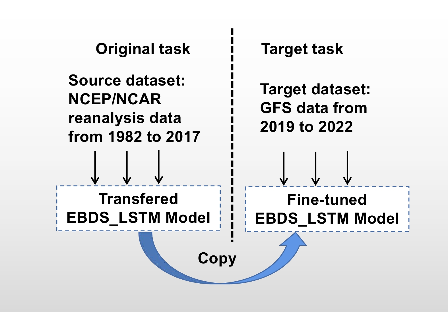
The transfer learning method (Pan and Yang, 2010; Bozinovski, 2020) was employed to address the data availability limitation in training deep learning neural networks. In this study, we primarily utilized the NCEP/NCAR reanalysis data to pre-train the model. After obtaining a well-performing pretrained model, we transferred it to the GFS real-time forecast data, which has a smaller data volume, for further training of the model (as shown in Fig. 3). The model training was performed using the Keras API under the Tensor Flow framework.

Figure 3. Transfer learning structure in the EBDS_LSTM model.
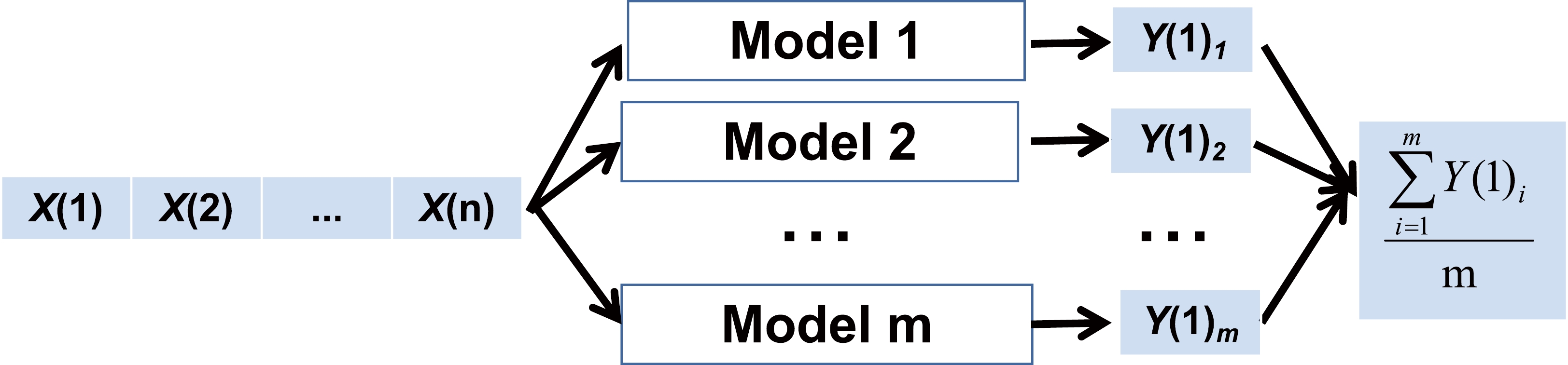
The commonly used regularization technique called “dropout” was employed to mitigate overfitting in the training process of deep-learning models (Srivastava et al., 2014). Since the results obtained from each training iteration may differ slightly due to factors such as different initial parameters, data perturbations, or the randomness of optimization algorithms, we trained 20 models and calculated their ensemble mean for final forecasts. The detailed framework is illustrated in Fig. 4.

Figure 4. Schematic of the ensemble forecast in the EBDS_LSTM model. X(n) indicates predictors as listed in Table 1 and Y(1)m indicates TC intensity, where m is the number of ensemble members (20).
-
Based on the selected predictors and the EBDS model in Eq. (1), a new TC intensity prediction scheme over the WNP was constructed using the TC best-track data and NCEP–NCAR reanalysis data during 1982–2016, and the CMA TC forecast track data and NCEP-GFS forecast data during 2019–21. Figure 5 summarizes the workflow in building the new TC intensity prediction scheme, termed the EBDS_LSTM scheme, which consists of two main parts: the model pretraining and transfer learning. The workflow for each part can be broadly divided into data preprocessing, hyperparameter optimization, model training, and validation and analysis of model performance. The data preprocessing was described in section 2. The modeling approach mainly involves stacking two LSTM layers, each with 128 neurons, followed by a fully connected layer with a single neuron as the output, representing the predictand at the required forecast time. Dropout layers are included between the layers and the dropout rates are separately set as a hyperparameter. The activation function used in the final fully connected layer is set as the second hyperparameter. Whether the former sequence of the predictand itself is included as a predictor (i.e., whether it is a rolling forecast) is controlled by a switch, which serves as the third hyperparameter. The model’s prediction target is set as a seven-day (five-day) forecast from 6 h to 168 h (120 h) at 6-h intervals for the reanalysis data (GFS forecast data), and the overall error in the test set is used to measure the model’s fitting and generalization ability.

Figure 5. Schematic of the EBDS_LSTM forecast scheme.
It is found that linear activation (tanh) functions are difficult to fit and result in larger prediction errors, while the rectified linear activation function (relu) might suffer from gradient vanishing that prevents proper model fitting. In contrast, the activation function elu (Exponential Linear Unit) shows better stability and smaller errors. Finally, two dropout rates of 0.4, the activation function elu, and the Adam optimizer with an initial learning rate of 0.001, which helps the model to automatically adjust the learning rate, were determined in the model. As mentioned above, in the original model based on the reanalysis data, the training dataset during 1982–2016 was used to train the relationship between predictors and
$E' $ , and the testing dataset in 2017 was built to predict$E' $ from 6 to 168 h at 6-h intervals. In the target model based on the GFS forecast data, the training dataset during 1982–2017 using the reanalysis data was adopted to pretrain the relationship between predictors and E', the GFS forecast dataset during 2019–21 was used to build the transfer learning model, and the target dataset during 2021–22 was built to predict E' from 6 to 120 h at 6-h intervals. To conduct independent forecasts, we excluded the cases from the training set when performing the experimental forecasts for those cases in 2021. Note that using these two sets of models, we can predict E' at each forecast time. The internal dynamical efficiency E* can be determined using Vmax and MPI at the initial time t0. Subsequently, we can predict Vmax for the subsequent moment t1, using the EBDS equation with a forward-time-differencing scheme. Based on the Vmax and MPI at t1, we are able to iteratively calculate E* for t1, and this procedure is repeated for subsequent time points. Through this iterative process, we achieve the prediction of the corresponding E*, E', and Vmax across various forecast times. -
The performance of the new scheme is evaluated based on independent forecasts for all TCs in 2017 using the reanalysis data and real-time forecasts for TC cases in 2021 and all TC cases in 2017 and 2022 based on the CMA TC track forecasts and the NCEP-GFS real-time forecast data. Note that the real-time GFS forecast data from 2017 was primarily used to determine whether transfer learning was necessary.
-
We first applied the newly developed scheme to the test set of the NCEP–NCAR reanalysis data in 2017. Figure 6a shows the root-mean-square errors (RMSEs) at different forecast times and the number of forecast samples of 7-day intensity forecasts from the EBDS_LSTM scheme and the 5-day forecasts from the CMA at 24-h intervals for all independent TC cases in 2017. In general, the RMSEs from the CMA forecasts increase with increasing forecast time. Interestingly, the RMSEs from our new model increase from 6 h to 72 h, but decrease rapidly afterwards. The performance of the EBDS_LSTM model is comparable to CMA within the forecast lead time of 72 h, while there are improvements of approximately 30% and 45.6% in the forecast accuracy at 96 h and 120 h, respectively. The good performance in medium and long-term forecasts demonstrates the superiority of the EBDS_LSTM scheme in capturing the major characteristics of TC intensity changes with the physical principles informed.
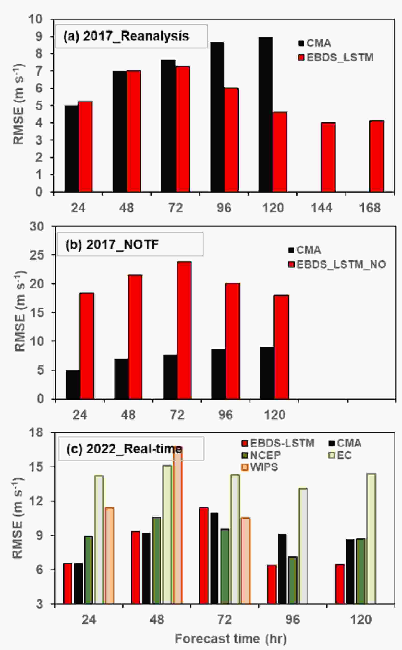
Figure 6. (a) Averaged RMSEs (m s−1) of the 7-day intensity forecasts from the EBDS_LSTM scheme (red bars) and averaged RMSEs of the 5-day forecasts from the CMA (black bars) at 24-h intervals for all independent TC cases in 2017 based on the NCEP–NCAR reanalysis data. (b) Averaged RMSEs (m s−1) of the 5-day real-time intensity forecasts at 24-h intervals from the EBDS_LSTM scheme and the CMA for all independent cases in 2017. (c) Averaged RMSEs (m s−1) of the 5-day real-time intensity forecasts at 24-h intervals for all independent cases in 2022 from the EBDS_LSTM scheme (red), CMA (black), NCEP-GFS (green), ECMWF (light green), and WIPS (orange). The EBDS_LSTM model was trained on NCEP–NCAR reanalysis from 1982 to 2016. For (a), predictions were made based on reanalysis; for (b), on GFS forecast data for the year 2017 without transfer learning; and for (c), on GFS forecast data for the year 2022, using transfer learning with GFS data during 2019–21.
The two most representative TCs, Noru (2017) and Lan (2017), were selected for case verification from all TC data in the test set of 2017 based on the following reasons: (1) they reached the highest maximum intensity among all TCs in the test set; (2) both had a duration of more than one week; (3) the entire lifespan of their formation and development was in accordance with cognition; (4) TC Noru (2017) underwent two rapid intensification stages, while TC Lan (2017) experienced rapid intensification and rapid weakening within a short period of time, representing different types of TC intensity changes. Figures 7a–d present the duration, track, and intensity of the two TCs. Noru formed as a tropical storm to the northeast of the Northern Mariana Islands on 20 July and reached its first peak intensity of 40 m s−1 on 24 July. After a brief weakening, it re-intensified and became a super typhoon on 30 July, with a maximum intensity of 52 m s−1, and then weakened back to a tropical storm before reaching Japan. Lan formed on 15 October in the southwestern NWP. It rapidly intensified into a super typhoon on 20 October, reaching its maximum intensity of 58 m s−1 a day later, and then rapidly weakened to a tropical storm and later dissipated within only two days.
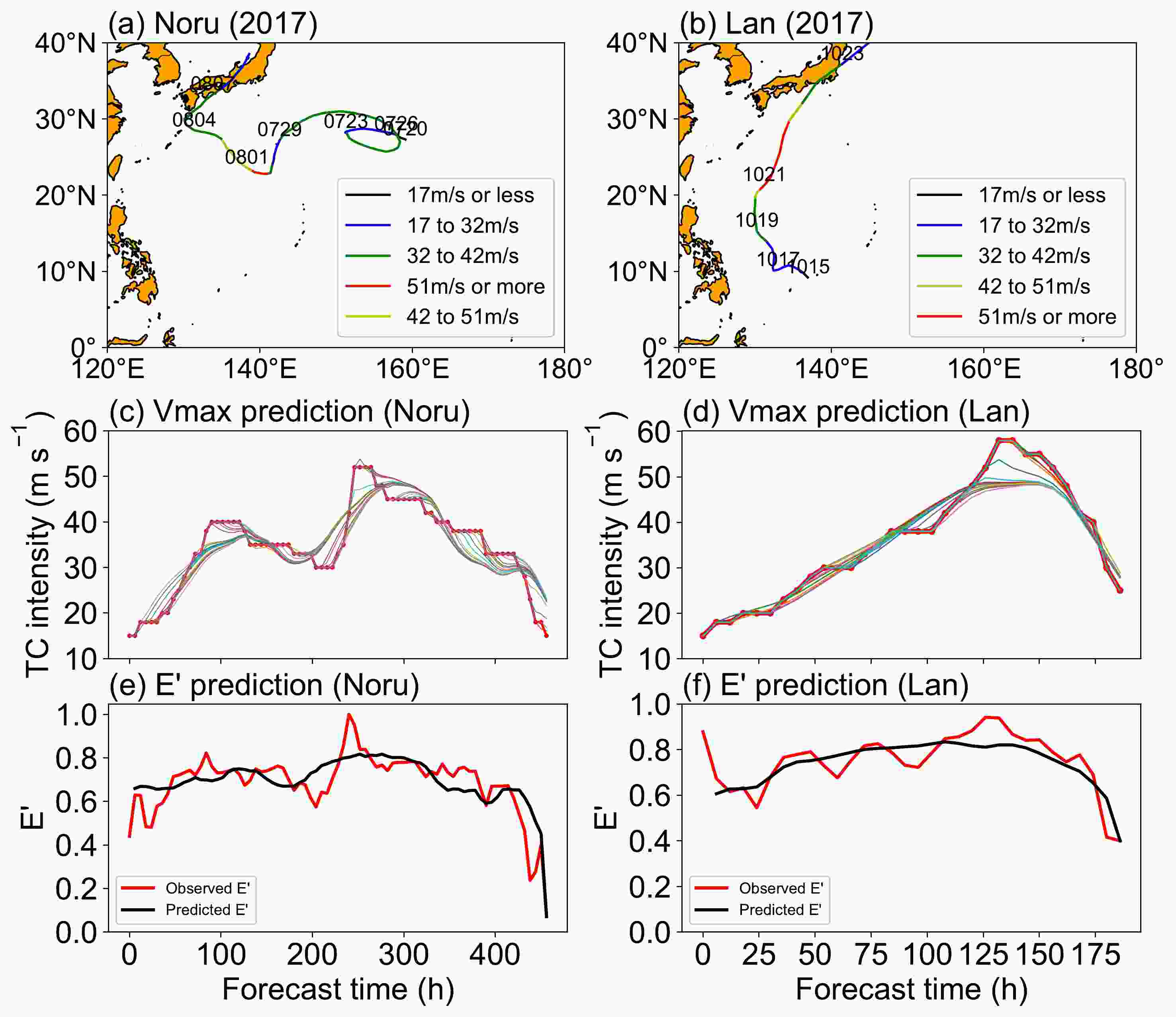
Figure 7. (a, b) Observed tracks and intensities of (a) Noru and (b) Lan in 2017. (c, d) The 7-day forecasts of the intensity for (c) Noru and (d) Lan at different forecast times with 6-h intervals based on NCEP–NCAR reanalysis data (dashed lines) and the corresponding CMA best-track intensity (red solid line). (e, f) Diagnosed (red) and predicted (black) dynamical efficiency factor E′ for (e) Noru and (f) Lan.
Figures 7c and d show the 7-day intensity forecasts for the two TCs from the EBDS_LSTM scheme based on the NCEP–NCAR reanalysis data, along with the best-track intensity. As expected, the EBDS_LSTM scheme reasonably captures the characteristics of intensity changes in different stages of the corresponding TCs. It not only accurately predicts the initial stage of intensification but also captures the rapid intensification and rapid weakening stages of both TCs. The EBDS_LSTM scheme also captures the peak intensity of the two TCs reasonably. Furthermore, we also calculated the RMSEs at different forecast times for the two cases and compared with the CMA forecasts (Table 2). The forecast errors from the CMA generally increase with increasing forecast time, while that from the EBDS_LSTM scheme remain small and even decrease at longer forecast times. Compared to the CMA forecasts, our EBDS_LSTM model improves by approximately 15.85%–52.6% for forecast times before 72 h. As for those beyond 72 h, our new scheme improves by about 31.1%–52.3%. This suggests that the accumulated errors may neutralize and lead to comparatively small errors in long-term forecasts because it is physics-based, and because of the use of the LSTM algorithm. In particular, the EBDS model yields promising results in long-term forecasts, which might be benefited by the constraints on physical equations, while it also achieves satisfactory short-term forecasts due to the powerful fitting and optimization capabilities of deep learning.
Forecast time (h) RMSE (m s−1) in Noru RMSE (m s−1) in Lan EBDS_LSTM CMA EBDS_LSTM CMA 24 4.23 7.32 3.82 5.40 48 4.48 8.84 4.16 5.36 72 4.36 9.20 4.40 5.23 96 4.29 9.00 4.85 7.04 120 4.31 8.14 5.36 9.51 144 4.45 - 3.64 - 168 4.61 - 2.83 - Table 2. RMSEs (m s−1) of intensity forecasts for Noru and Lan in 2017 at 24, 48, 72, 96, 120, 144, and 168 h from the EBDS_LSTM scheme and the CMA 5-day forecasts. Smaller RMSEs between the two methods are shown in boldface.
Figures 7e and f illustrate the diagnosed and predicted environmental dynamical efficiency (E') for the two TCs. In both cases, the diagnosed E' exhibits a similar evolution to the TC intensity but with a lead of 6 hours. The E' for Noru exhibits a prominent bimodal structure with two growth and decay stages, albeit with some jagged fluctuations, while Lan experiences one peak with some relatively large fluctuations. This suggests that the effect of E' is vital. For the predicted E', the model generally reproduces well the change in the diagnosed E', although some underestimations are visible when the TC is near its peak intensity. Note that the predicted E' and TC intensity are much smoother than the diagnosed E' and best-track intensity. This can be attributed partly to the noise in observational data, and partly to the model’s adjustments during training, which aim to minimize overfitting by targeting more generalized patterns.
-
Prior to utilizing GFS forecast data in our final real-time forecast model, we assessed the necessity of transfer learning. Here, the EBDS_LSTM was trained on reanalysis data from 1982 to 2016, and then made forecasts directly using GFS forecast data for 2017, with results shown in Fig. 6b. As anticipated, the forecast error at each forecast time exceeded 15 m s−1, significantly higher than that from the CMA forecast. It strongly suggests the necessity and importance of implementing transfer learning for tuning the model.
Furthermore, based on the pretrained EBDS_LSTM scheme using the NCEP–NCAR reanalysis data, the scheme was further trained using the GFS forecast data from 2019 to 2021, except for two testing cases of Typhoon Surigae (202102) and Typhoon Nyatoh (202121), which experienced rapid intensification and were selected for real-time forecast verification. Figures 8a and b show the observed tracks and intensities of Surigae and Nyatoh. Surigae formed as a tropical storm over the WNP on 13 April and rapidly intensified within a few days to become a super typhoon with a peak intensity of 68 m s−1 on 17 April. It approached the Philippines and turned northeastward over the ocean, and then gradually weakened. Nyatoh formed on 30 November in the southwestern WNP, near the Philippines and north of Indonesia. After a few days of slow intensification, it rapidly intensified into a super typhoon with a maximum intensity of 55 m s−1 on 3 December. It then quickly weakened to a tropical storm and dissipated in a day.
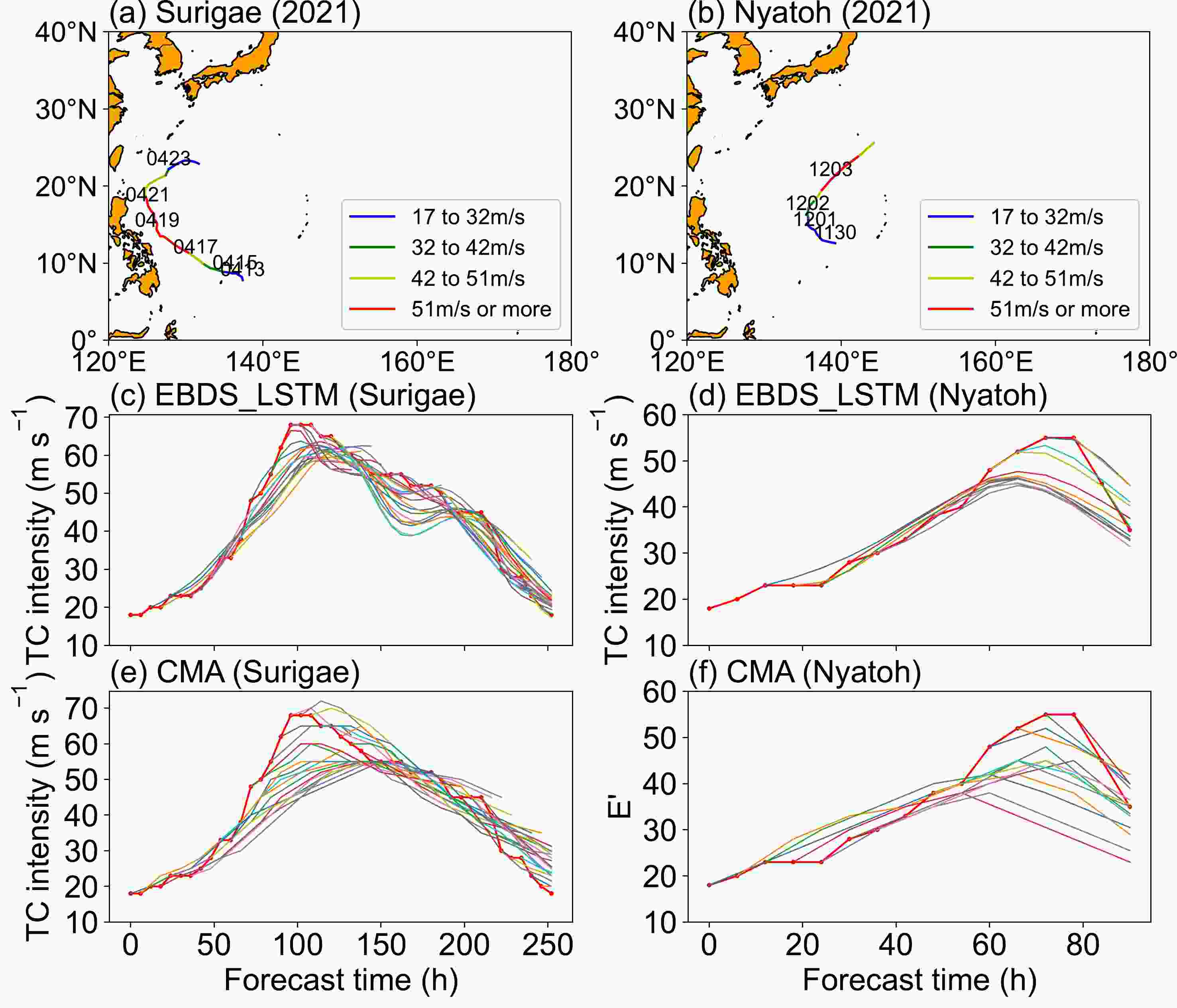
Figure 8. (a, b) Observed tracks and intensities for (a) Surigae and (b) Nyatoh in 2021. (c–f) The 5-day forecasts of the intensity for (c, e) Surigae and (d, f) Nyatoh at different forecast times with 6-h intervals from (c, d) the EBDS_LSTM forecasts (dashed lines) and (e, f) the CMA forecasts (dashed lines). In (c–f), red solid lines indicate the corresponding CMA best-track intensity.
Figures 8c and d show the intensity forecasts from the EBDS_LSTM scheme based on predictors obtained from the GFS real-time forecast data and the real-time track forecasts from the CMA. The EBDS_LSTM scheme captures well the characteristics of intensity changes in almost all stages of the two TCs, including the magnitude of intensification and weakening rates. It accurately captures both the initial intensification stage and the rapid intensification and rapid weakening stages of the two TCs. Compared with that from the CMA, forecasts from the EBDS_LSTM scheme show better transitions in the TC development stages and overall better skill in predicting the peak intensity. We also calculated the corresponding RMSEs of the forecasts for the two cases (see Table 3). The RMSEs of the CMA forecasts exhibit an increase with increasing forecast lead time, reaching a maximum at 72 h, followed by a slight decrease. In contrast, the RMSEs of the forecasts from the EBDS_LSTM scheme are small at all lead times, showing no significant increase with increasing forecast time. This indicates that the EBDS_LSTM scheme performs better in both short-term and long-term forecasts for both TCs than the CMA forecasts.
Forecast Time (h) RMSE (m s−1) in Surigae RMSE (m s−1) in Nyatoh EBDS_LSTM CMA EBDS_LSTM CMA 24 4.23 5.53 3.82 6.60 48 4.48 8.64 4.16 11.21 72 4.36 9.73 4.40 13.88 96 4.29 9.12 4.85 − 120 4.31 7.68 5.36 − Table 3. RMSEs (m s−1) of intensity forecasts for Surigae and Nyatoh in 2021 at 24, 48, 72, 96 and 120 h forecasts from the EBDS_LSTM method and the CMA 5-day forecasts. Smaller RMSEs between the two methods are shown in boldface.
To demonstrate the overall good performance in the forecast mode of our developed EBDS_LSTM scheme, we also conducted retrospective forecasts for all 23 TCs in 2022 (excluding Typhoon 2211 because of missing data). Figure 6c shows the RMSEs of 5-day intensity forecasts from the EBDS_LSTM scheme and a comparison with those from several main forecast agencies. One notable feature is that, except for the 72-h forecast, the EBDS_LSTM scheme performs better at all other forecast times. Particularly at the longer lead times of 96 h and 120 h, the EBDS_LSTM scheme has smaller forecast errors, with a 10% and 25% improvement over the NCEP-GFS forecasts and a 51% and 55% improvement over the ECMWF forecasts, respectively. Additionally, it is worth mentioning that despite utilizing the same predictors as WIPS, the EBDS_LSTM scheme exhibits a significant improvement. This suggests that the EBDS_LSTM model has the potential to contribute to improving TC intensity forecasts over the WNP.
-
We introduced a new prediction scheme for TC intensity over the WNP based on the cutting-edge EBDS model, together with the LSTM framework of deep learning. The latter is used to predict the environmental dynamical efficiency in the EBDS model. Since the LSTM algorithm exhibits an outstanding performance for time series predictions, it is suitable for use in the prediction of TC intensity. We also used other approaches in constructing the new prediction scheme, including optimization and tuning of model hyperparameters, transfer learning, and the ensemble method.
Independent forecasts for all TCs in 2017 based on the NCEP–NCAR reanalysis data show that the EBDS_LSTM scheme has better skill in predicting TC intensity over the WNP than the CMA’s official operational forecasts, which is one of the best forecasts for the basin. The good performance of the newly developed EBDS_LSTM scheme for “real-time” forecasts was demonstrated with two TC cases in 2021 and all TC cases in 2022. The new scheme shows better prediction skill than the official prediction from the CMA and other state-of-art statistical and dynamical forecast systems, particularly for long lead-time forecasts of 96 h and 120 h.
In comparison with traditional dynamical system model approaches, such as the LGE model, the EBDS_LSTM scheme is physics-based and shows superior forecasting capabilities, significantly reducing prediction errors, and offering a new independent TC intensity prediction scheme for the WNP. We also compare the current model to other popular deep-learning methods, including early attempts with artificial neural networks and more recent advancements using RNNs, multi-module-task models, LSTM, and Pangu-Weather (Pan et al., 2019; Baik and Paek, 2000; Yuan et al., 2021; Wang et al., 2022; Bi et al., 2023). These studies illustrate incremental improvements in TC intensity prediction, and generally show similar forecasting skill within 48 h to those in our new model. However, these methods highlight limitations such as forecast duration and a disregard for the underlying physical processes. As such, our model shows better skill for long lead-time forecasts (96 h and 120 h), aligning with the physical principles of TC intensity change.
We would like to point out that, although the scope of this study has focused on prediction of TC intensity over the WNP, the new scheme can be potentially applied to other TC basins, such as the North Atlantic and eastern North Pacific, because the EBDS model is physics-based, which is independent of the basin. In addition, through sensitivity experiments by varying different environmental variables, the EBDS_LSTM scheme can also be used to identify key factors related to the rapid intensification and rapid weakening phases of TCs. This will potentially not only progressively enhance the forecasting skill, but also help explore unknown physical mechanisms from a theoretical perspective, bridging the gap between the black box of deep learning and practical applications of weather forecasting in a more transparent way.
Acknowledgements. The authors appreciate Yinglong XU and Shijin YUAN for their constructive comments. This work was supported by the National Key R&D Program of China (Grant No. 2017YFC1501604) and the National Natural Science Foundation of China (Grant Nos. 41875114 and 41875057). The CMA best-track TC dataset was downloaded from
http://tcdata.typhoon.org.cn/ . The official real-time forecast data of the CMA and the GFS forecast fields were derived from the TC operational database at STI. The NCEP–NCAR reanalysis data were downloaded fromhttps://www.esrl.noaa.gov/psd/data/gridded/data.ncep.reanalysis.html .
| Predictor | Units | Description |
| VWS | m s−1 | Averaged vertical wind shear between 200 and 850 hPa within a radius of 5° of the TC center |
| AU | m s−1 | Averaged zonal wind at 200 hPa within a radius of 5° of the TC center |
| AV85 | s−1 | Averaged absolute vorticity at 850 hPa within an annulus area between radii of 5° and 10° of the TC center |
| DIV85 | s−1 | Averaged divergence at 850 hPa within an annulus area between radii of 5° and 10° of the TC center |
| DIV20 | s−1 | Averaged divergence at 200 hPa within an annulus area between radii of 5° and 10° of the TC center |
| H50 | gpm | 500-hPa geopotential height at the TC center |
| VOR85_lon | ° | Longitude of the greatest vorticity at 850 hPa in the range of 2° (4°) of the TC center at 0−24 h (> 24 h) forecasts |
| VOR85_lat | ° | Latitude of the greatest vorticity at 850 hPa in the range of 2° (4°) of the TC center at 0−24 h (> 24 h) forecasts |
| RH8570 | % | Averaged relative humidity at 850–700 hPa within an annulus area between radii of 5° and 10° of the TC center |
| RH5030 | % | Averaged relative humidity at 500–300 hPa within an annulus area between radii of 5° and 10° of the TC center |
| MPI | m s−1 | Maximum potential intensity estimated using the SST averaged within a radius of 300 km from the TC center |


 AAS Website
 AAS WeChat