Correcting Climate Model Sea Surface Temperature Simulations with Generative Adversarial Networks: Climatology, Interannual Variability, and Extremes

Climate model simulations play an indispensable role in contemporary climate science, serving as fundamental resources for climate change detection, attribution, and projection. Their simulations, especially from the Coupled Model Intercomparison Project (CMIP), underpin the assessments conducted by the Intergovernmental Panel on Climate Change (IPCC), offering comprehensive evaluations and pivotal references that support the advancement of global climate science and guide critical decision-making (Taylor et al., 2012; Eyring et al., 2016). However, the utility of CMIP models in both detection and attribution of climate change, as well as climate projections, is significantly impeded by various persistent model biases (Li and Xie, 2012, 2014; Zheng et al., 2012; Liu et al., 2014; Tao et al., 2018; Jiang et al., 2019, 2021; Capotondi et al., 2020; Danabasoglu et al., 2020).

Among these biases, a prominent concern centers on the representation of sea surface temperatures (SSTs) in coupled general circulation models (CGCMs), especially the persistent cold tongue bias found in the equatorial Pacific (Li and Xie, 2012, 2014; Zheng et al., 2012). This phenomenon, characterized by a cold bias in the climatological SSTs, has long perplexed the climate community due to its potential repercussions on climatological precipitation patterns and the accurate simulation of the El Niño-Southern Oscillation (ENSO), thereby affecting the fidelity of global climate simulations (Tao et al., 2018; Jiang et al., 2019; Tang et al., 2023). Additionally, substantial biases manifest themselves at interannual scales, with ENSO SST variability exhibiting an excessive westward extension into the equatorial western Pacific, consequently impacting ENSO decay processes and regional climate variability. These biases, commonly present in most of the CMIP models, are hardly canceled out, even by multi-model means (Huang and Ying, 2015; Jiang et al., 2021; Tang et al., 2023), thus impacting historical simulations and future projections.

Efforts to rectify these climate model biases have spawned the development of various methodologies. Traditional methods predominantly center around the local adjustment of specific statistical characteristics. These adjustments typically target parameters like the mean and variance (involving variance adjustment; Chen et al., 2011, 2013; Teutschbein and Seibert, 2012; Li et al., 2019), and frequency distributions (via techniques like quantile mapping; QM; Jakob Themeβl et al., 2011). However, these approaches fall short of providing precise corrections for model errors at the daily timescale and in dynamical climate variabilities. Traditional methods primarily focus on specific statistical features or target adjustments at individual grid points and can by design not correct spatial patterns (Hess et al., 2022, 2023).

The challenge of climate model bias correction is exacerbated by the internal variability of the Earth system, characterized by inherent nonlinearity (Hawkins and Sutton, 2011; Deser et al., 2012, 2016; Hu et al., 2019; Wang et al., 2020). In particular, discrepancies arise due to internal variability in model simulations and observations at corresponding times. Consequently, discerning whether disparities between model fields and observational datasets arise from internal variability or genuine model biases poses a substantial challenge; identifying and, on that basis, correcting the bias for a particular day in model data is inherently difficult. This presents a challenge when trying to employ traditional statistical methods and supervised learning techniques to correct model simulations.

The advent of deep learning, particularly the development of unsupervised and semi-supervised learning techniques, has introduced novel avenues for addressing climate model biases. Generative Adversarial Networks (GANs), pioneered by Goodfellow et al. (2014), leverage a generator-discriminator framework to generate images that are in their characteristics and statistical properties virtually indistinguishable from target images. Subsequently, Hoffman et al. (2017), Yi et al. (2017), and Zhu et al. (2017) expanded upon the GAN methodology, introducing the Cycle-consistent GAN (CycleGAN), which incorporates a cycle-consistent loss to facilitate the bidirectional transformation of data styles. Pan et al. (2021) have explored the application of this method to rectify precipitation data in CGCM simulations, yielding promising results in correcting precipitation biases in the United States. Moreover, the extension of this method to global precipitation simulations demonstrated its efficacy in correcting spatial patterns and in ameliorating the Pacific double Intertropical Convergence Zone (ITCZ) bias (Hess et al., 2022, 2023), a prevalent issue across most CGCMs. These applications have predominantly concentrated on evaluating the enhancement of fundamental statistical aspects of precipitation.

The critical inquiry here is whether this method can also address bias-correct modeled SST fields. Furthermore, it is unclear whether it can correct the dynamical oceanic modes and adapt to variations driven by distinct physical mechanisms at various timescales. These unclarified issues presently lack a definitive resolution.

In this paper, we employ a CycleGAN-based approach to correct global daily SST fields to address these concerns. We find that our method not only addresses biases at climatological averages but also tackles errors associated with ENSO, the Indian Ocean Dipole (IOD), and SST extremes. The remainder of this paper is structured as follows. Section 2 provides introductions of the datasets and methodology employed, section 3 unveils the primary results, and section 4 discusses and summarizes our findings.

We employ daily surface temperature (ST) data from the National Center for Environmental Prediction-Department of Energy Atmospheric Reanalysis (NCEP; Kanamitsu et al., 2002) at a resolution of 2.5° × 2.5° for the period 1950–2014. Modeled daily ST fields from 1950–2014 are obtained from the Community Earth System Model 2 (CESM2; Danabasoglu et al., 2020), a widely used and well-organized model, which can be considered a state-of-the-art climate model. The global gridded monthly SST datasets from Extended Reconstructed Sea Surface Temperature (ERSST.v5; Huang et al. 2017), the NOAA 1/4° Daily Optimum Interpolation SST (OISST; Huang et al., 2021), and the Hadley Centre Global Sea Ice and SST (HadISST) are utilized. These three SST datasets and NCEP ST, ranging from 1991−2014, are utilized for model testing. All datasets are interpolated to a resolution of 2.5° × 2.5°.

To extract ENSO-related SST variability, we utilize the unstandardized Niño-3.4 index. This index is defined as the SST anomalies (SSTA) averaged over the region between 5°S–5°N, and 120°–170°W from December to February (DJF). We performed a regression analysis of this unstandardized Niño-3.4 index on the interannual SSTAs, thus revealing the underlying ENSO-driven SST variability. The IOD SST is obtained in a similar way to that of the ENSO SST but uses the Dipole Mode Index, defined as the anomalous SST gradient between the western equatorial Indian Ocean (50°–70°E and 10°S–10°N) and the southeastern equatorial Indian Ocean (90°–110°E and 10°S–0°) during September–October–November (SON).

CycleGAN is a groundbreaking deep-learning model designed for unpaired image-to-image translation. It enables the transformation of images from one domain to another even when paired training data is unavailable (Zhu et al., 2017), such as in the case addressed in the present study. Unpaired image-to-image translation involves the mapping of images from one domain (the source domain, denoted by X) to another (the target domain, denoted by Y) without requiring a direct one-to-one correspondence between the images in the two domains. In our case, we apply the principles of unpaired image-to-image translation for the correction of CGCM daily SST data. Specifically, we consider the CESM2 SSTs as domain X and NCEP STs as domain Y. The training and validation data comprises the CESM2 and NCEP ST data from 1950 to 1990, while the testing data spans from 1991 to 2014. A normalization process is employed to scale the data.

Figure 1 gives the schematic of the CycleGAN. Within the CESM2, biases exist in the internal variability and externally forced responses within model simulations on any given day. However, the internal variability in observations on the same day may not correspond to that in the model. For example, the model might simulate an El Niño year, while observations indicate a La Niña year. Therefore, directly adjusting the model to match the observational state would be profoundly inaccurate. Our goal is to eliminate biases in the internal variability and externally forced responses while simultaneously preserving the model's internal variability (e.g., the ENSO phase).

Figure 1.  (a) Schematic of the CycleGAN. (b) The details of ResNet, which has nine residual blocks. (c) The details of the first residual block, and (d) other blocks.

To achieve this objective, a generator [G(x)] and a discriminator are first employed in this model (Fig. 1a). The primary function of the generator is to transform the CESM2 data to match the observational SST, while the discriminator assesses whether the generated outcomes originate from observations. A balance between these two components yields the best results, wherein the discriminator should be incapable of distinguishing between images generated by the generator and observations. This phase aids in correcting the GCM simulations. Subsequently, a secondary generator [F(y)] and a discriminator are utilized to retain the internal variability. The secondary generator, F(y), is tasked with reconverting the previously generated images back into the original CESM2 data. This process ensures that the generated images by G(x) retain the essential characteristics of CESM2. From a mathematical perspective, the architecture of F(y) ensures a bidirectional mapping between CESM2 and the observational data. In a certain context, this secondary generator facilitates the preservation of internal variability within CESM2, as internal variability is a predominant aspect of a daily timescale.

The loss function of this model is as follows:

The loss includes the adversarial loss of X→Y [$ {\mathcal{L}}_{\mathrm{G}\mathrm{A}\mathrm{N}}\left(G,{D}_{Y},X,Y\right) $, see Eq. (2)], Y→ X [$ {\mathcal{L}}_{\mathrm{G}\mathrm{A}\mathrm{N}} \left(F, {D}_{X}, Y,X\right) $, see Eq. (3)], the consistency loss [$ {\mathcal{L}}_{\mathrm{c}\mathrm{y}\mathrm{c}}\left(G,F\right) $], and the identity loss [$ {\mathcal{L}}_{\mathrm{i}\mathrm{d}}\left(G,F\right) $]. G denotes a generator that tries to generate images G(x) that are indistinguishable from those in Y, F represents a generator that tries to generate images F(y) similar to those in X. $ {D}_{Y} $ and $ {D}_{X} $ denote the discriminators aiming to distinguish between G(x) and y, and F(y) and x, respectively.

Equations (2) and (3) show the adversarial loss, where $ \mathbb{E} $ means the expected value. Moreover, following Zhu et al. (2017), the consistency loss and identity loss [Eqs. (4) and (5)] are further added to help retain the internal variability and avoid introducing additional bias, the weights of these terms are controlled by $ {\lambda }_{c} $ and $ {\lambda }_{i} $, which are set to 10 and 0.5, respectively.

The generative networks consist of three components: down-sampling with two convolutional layers, followed by nine residual blocks comprising a total of 21 convolutional layers, and finally two up-sampling layers (as depicted in Fig. 1). The first residual block, represented in Fig. 1c, contains five convolutional layers, while the subsequent blocks, as shown in Fig. 1d, each consist of two convolutional layers. This deep generative network helps generate finer SST images. The architecture of the discriminator aligns with the model presented by Zhu et al. (2017). Gradient clipping is employed to optimize the training of the model. In training the GAN, the Wasserstein loss is utilized, chosen for its known stability (Arjovsky et al., 2017).

In the following development, we employ linear regression and composite analysis and determine the statistical significance according to a two-tailed Student’s t-test.

Figure 2 presents a qualitative comparison of daily ST on the same date (3 November 2004). CycleGAN essentially preserves most features present in CESM2 results, notably the La Niña-like SSTAs (Figs. 2b, c), while also exhibiting a greater resemblance to observations (Figs. 2a, c). This improvement is particularly notable in regions such as the tropical Atlantic, South Africa, and western South America. This comparison effectively signifies that the data post-processed by CycleGAN, in addition to correcting model outcomes, preserves the internal variability of the model.

Figure 2.  Qualitative comparison of the intermittency in daily ST on the same date (3 November 2004), from the (a) observation, (b) CESM2 model, and (c) CycleGAN-based post-processing. White contour lines (with an interval of 1 K) denote the monthly SSTAs in November 2004.

In the subsequent analysis, we evaluate the correction from three key perspectives: climatology, interannual variability, and extreme events. To validate the effectiveness of the correction, we performed comparisons between results obtained from CESM2, GAN-corrected SSTs, and four reference datasets (HadISST, ERSST, NCEP, OISST).

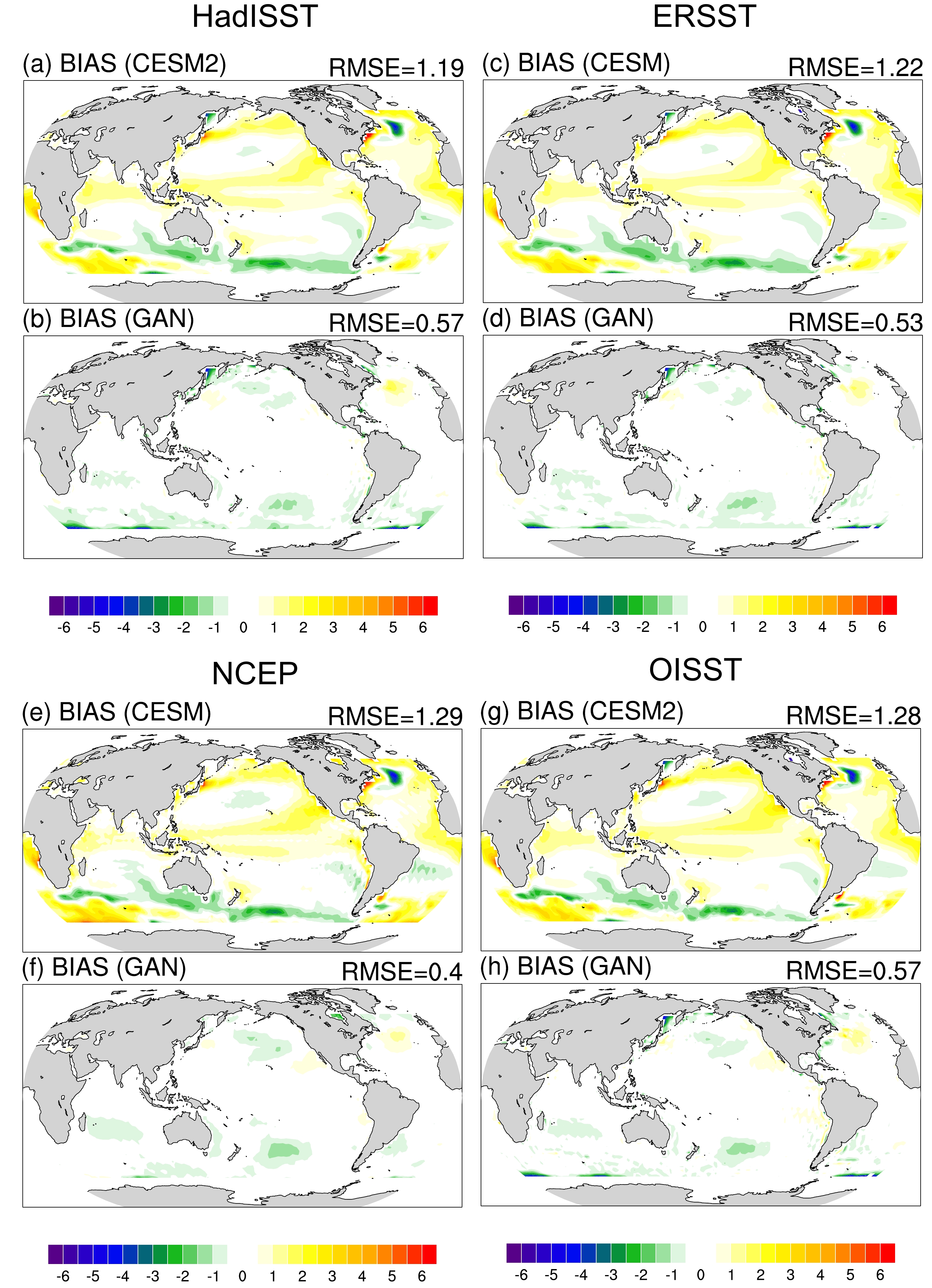
Figure 3 illustrates the disparities between CESM2 model data, GAN-corrected outcomes, and observational datasets. Overall, CESM2 displays a substantial warm bias when compared to the four SST datasets. There is a distinct dipole bias in SSTs in the North Atlantic, particularly along the Gulf Stream and North Atlantic Current, where warm and cold biases coexist in proximity. A similar dipole bias is observed in the Southern Ocean at mid-to-high latitudes. Notably, prominent warm biases are noticeable near eastern boundary upwelling regions, encompassing areas close to California, South America, and Africa (Figs. 3a, c, e, g). These biases are likely associated with discrepancies in wind stress patterns within these regions and the spatial resolution of the model (Capotondi et al., 2020). Additionally, a significant warm bias is evident in the tropical Pacific. This warm bias is distinct from the well-known cold tongue bias observed in most CMIP5 models and even differs from CESM1, signifying disparities between CESM2 and its predecessors, a feature also acknowledged in previous CESM2 assessment studies (e.g., Capotondi et al., 2020).

Figure 3.  The disparities between climatological annual mean SSTs in (a, c, e, g) CESM2 simulations, (b, d, f, h) GAN-corrected SSTs, and (a, b) HadISST, (c, d) ERSST, (e, f) NCEP, (g, h) OISST.

After the correction by the CycleGAN, there is a substantial reduction in the bias in the climatological SSTs (Figs. 2b, d, f, h). The dipole biases in the North Atlantic and the Southern Hemisphere are notably reduced. Only minor cold biases persist in the vicinity of eastern Africa and to the east of New Zealand. Furthermore, the warm biases in the tropical Pacific are significantly attenuated. The overall bias diminishes from 1.25°C (1.19°C to 1.28°C) in CESM2 to 0.52°C (0.4°C to 0.57°C). Through a comparative analysis involving four sets of SST data, we find that the biases, both in magnitude and spatial pattern, are highly consistent across the different datasets. This robust agreement underscores the reliability of our evaluation. In addition, CycleGAN exhibits clear advantages over traditional methods. We compare its performance with the widely utilized modified QM approach (Jakob Themeßl et al., 2011; Bai et al., 2016), widely employed for the correction of historical simulations and future projections within CMIP. When applied to SST correction, the modified QM yields an error of 0.6, which is inferior to the results obtained by CycleGAN (Fig. 4). It is noteworthy that the performance of QM and CycleGAN is remarkably close in tropical regions, and in the North Pacific, QM even outperforms it in the latter. However, QM exhibits larger errors in the high-latitude regions of the Southern Ocean.

Figure 4.  The disparities between climatological annual mean SSTs in (a) CESM2 simulations, (b) QM-corrected SST, and NCEP.

The errors calculated based on the NCEP data align closely with those from other datasets, further affirming the suitability of this dataset for model training. Given the substantial convergence in results across three SST datasets (HadISST, ERSST, OISST), for the sake of brevity, we will exclusively employ HadISST as the observational reference in the subsequent sections.

In addition to addressing biases at the climatological scale, an essential aspect of climate model correction, and perhaps even more crucial, is the capability to simulate the interannual dynamical variability such as ENSO and the IOD. The accurate representation of these variabilities directly influences the ability to capture global and regional climate variability. Figure 5 displays the DJF ENSO SSTA, in observations, CESM2, and CycleGAN-corrected SST. Notably, CESM2 exhibits an excessive westward bias in the equatorial Pacific, with a pronounced warm bias in the equatorial western Pacific. This bias is well-known and prevalent in many models, constituting a common bias in most CMIP5 and CMIP6 models (Tao et al., 2015, 2018, 2019; Jiang et al., 2021). It is worth noting that this substantial warm bias in ENSO SSTAs can be primarily attributed to the climatological cold tongue bias (Li and Xie, 2012, 2014; Jiang et al., 2021). The cold tongue bias manifests as a phenomenon in the model simulation, signifying that the climatological annual mean (SST) in the central-eastern tropical Pacific is colder than observed. This is characterized by an excessively strong and westward-extending cold tongue in the equatorial Pacific. The presence of the cold tongue bias can influence SSTAs in this region through its impact on temperature advection and other related processes. Despite the warm bias in the western Pacific in CESM2, its climatology also exhibits a warm bias. This suggests that the warm bias in the western Pacific of CESM2 may be attributed to other mechanisms.

Figure 5.  ENSO-related SSTAs in (a) observation, (b) CESM2, (c) QM, and (d) CycleGAN. Stippling indicates where the regressions are significant at the 95% confidence level, based on a Student’s t-test. The hatched areas represent significant differences in El Niño composite SSTs within the CycleGAN-corrected fields compared to CESM2. The black contour line denotes +0.2 K in observations.

The modified QM method exhibits limited efficacy in the correction of ENSO SSTs. Its RMSE and PCC closely align with CESM2, and is ineffective in addressing distributional biases, such as excessive westward bias (Fig. 5c). After correction by the CycleGAN, the warm bias is greatly diminished in the equatorial-western Pacific, with its intensity comparable to observations. Furthermore, the warm bias in the central and eastern Pacific, as observed in CESM2, is also notably reduced. A significance test was performed for composite El Niño SSTs, revealing significant differences between CESM2 and the CycleGAN-corrected results in several regions, including the equatorial western Pacific, the equatorial sides of the central Pacific, and the tropical eastern Pacific (Fig. 5d). This indicates a statistically reliable improvement by the CycleGAN in addressing warm biases in CESM2. Overall, upon applying the correction, we observe a significant reduction in the excessive westward bias of ENSO SST variability, with the distribution closely resembling observations. The RMSE decreases from 0.14 in CESM2 to 0.06, and the PCC increases from 0.89 to 0.95, corresponding to a 57% reduction and a 6.7% improvement, respectively.

Figure 6 shows the standard deviation of SSTs in the Indian Ocean and the IOD SSTA. In the CESM2 simulation, there is a significant overestimation of variability in the southeastern and western equatorial Indian Ocean, with the center of variability extending too far westward in the southeastern Indian Ocean when compared to observations. Similar to its limited efficacy in ENSO correction, the modified QM method demonstrates constrained effectiveness in the correction of SST variability. While the CycleGAN markedly reduces the biases in the southeastern and western equatorial Indian Ocean compared to CESM2, the excessive westward extension is substantially attenuated. The IOD mode also exhibits bias, for example, the standard deviation of SSTs (Fig. 6f). In CESM2, the IOD SSTA in the southeastern Indian Ocean is significantly stronger and extends too far westward compared to observations. In observations, negative anomalies roughly extend to 85°E, while in CESM2, the negative anomaly extends to around 70°E. CycleGAN successfully reduces this bias, with the negative anomaly located east of 80°E, significantly closer to observations. As such, its performance is noticeably superior to modified QM, with the latter making only marginal adjustments to the intensity of SSTA. The RMSE of CycleGAN is substantially decreased compared to CESM2, from 0.34 to 0.21, while the PCC increases from 0.82 to 0.92.

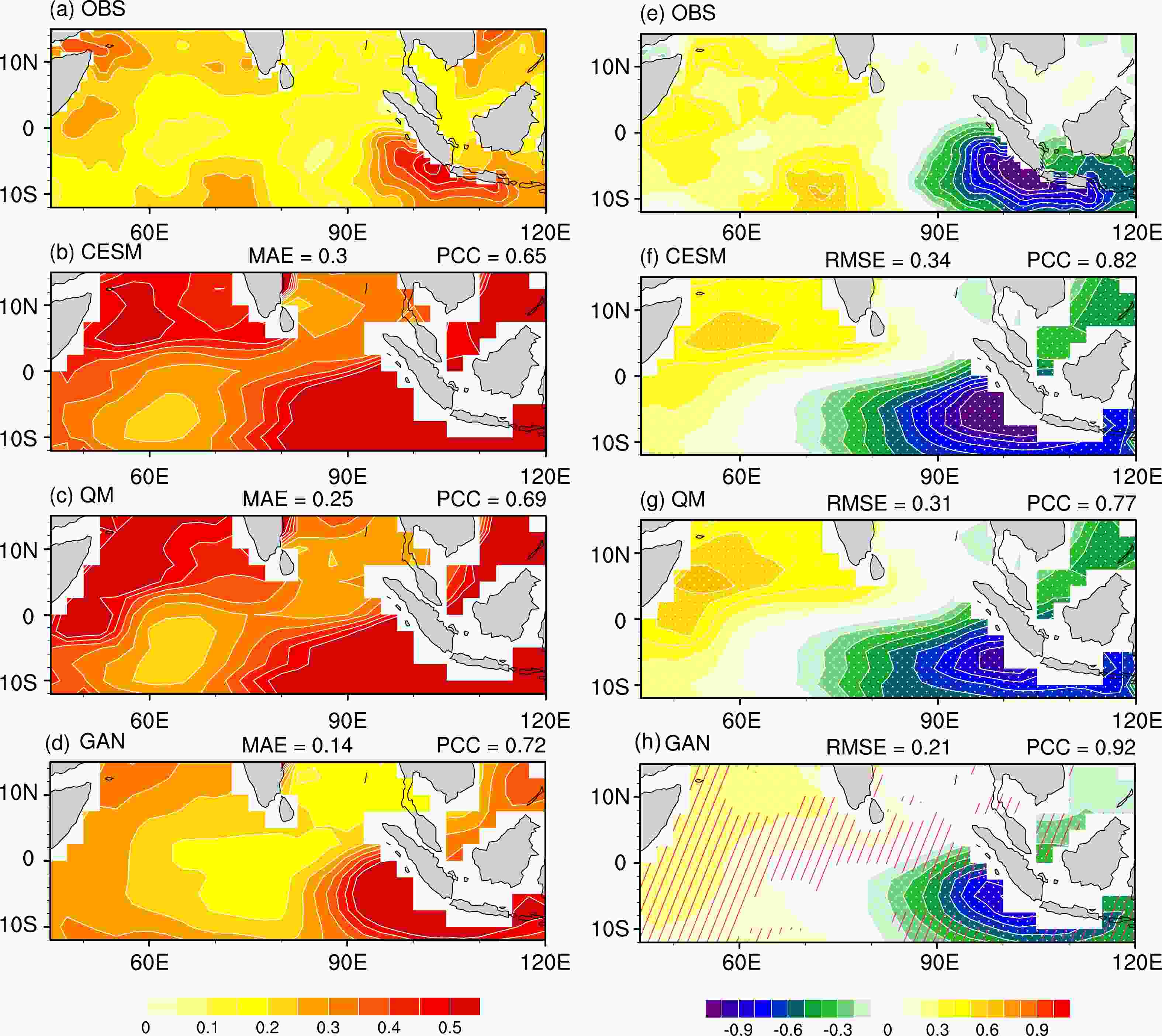
Figure 6.  (Left) The standard deviation of SST and (b) the IOD-related SSTA during SON in (a, e) observation, (b, f) CESM2, (c, g) QM, and (d, h) CycleGAN, respectively. Stippling indicates the regressions are significant at the 95% confidence level, based on a Student’s t-test. The hatched areas represent significant differences in positive IOD composite SSTs within the CycleGAN compared to CESM2.

In addition to interannual dynamical variability, marine heatwaves are a recent focus in oceanic research. Frequent marine heatwaves significantly impact marine ecosystems, particularly marine fisheries and coral reefs (Oliver et al., 2017, 2018, 2021; Holbrook et al., 2019; Liu et al., 2022, 2023). We primarily use the 95th percentile of daily SSTA to quantify SST extremes and evaluate the performance of CESM2 and the GAN-correction in representing them. To conduct the evaluation, we utilized NCEP data spanning from 1991 to 2014 for testing. Figure 7 illustrates the 95th percentile of NCEP, CESM2, and CycleGAN-corrected SSTA, respectively. In the NCEP data, regions with high values of the 95th percentile are concentrated in the western boundary current extension regions, the central and eastern equatorial Pacific, and the northeast Pacific Ocean, consistent with previous studies (Chen et al., 2014; Echevin et al., 2018; Oliver et al., 2017, 2021). When compared to NCEP, the spatial distribution of the 95th percentile in CESM2 is generally similar. However, CESM2 significantly overestimates the intensity of extreme SSTAs in the central and eastern tropical Pacific while underestimating it in the northwest Pacific. In contrast, CycleGAN-corrected extreme SSTA shows better agreement with observations in terms of intensity and spatial distribution. The PCC improves from 0.56 to 0.88, and the RMSE decreases from 0.5 to 0.32, slightly outperforming those obtained with modified QM.

Figure 7.  Same as in Fig. 5, but for the 95th percentile of SSTAs.

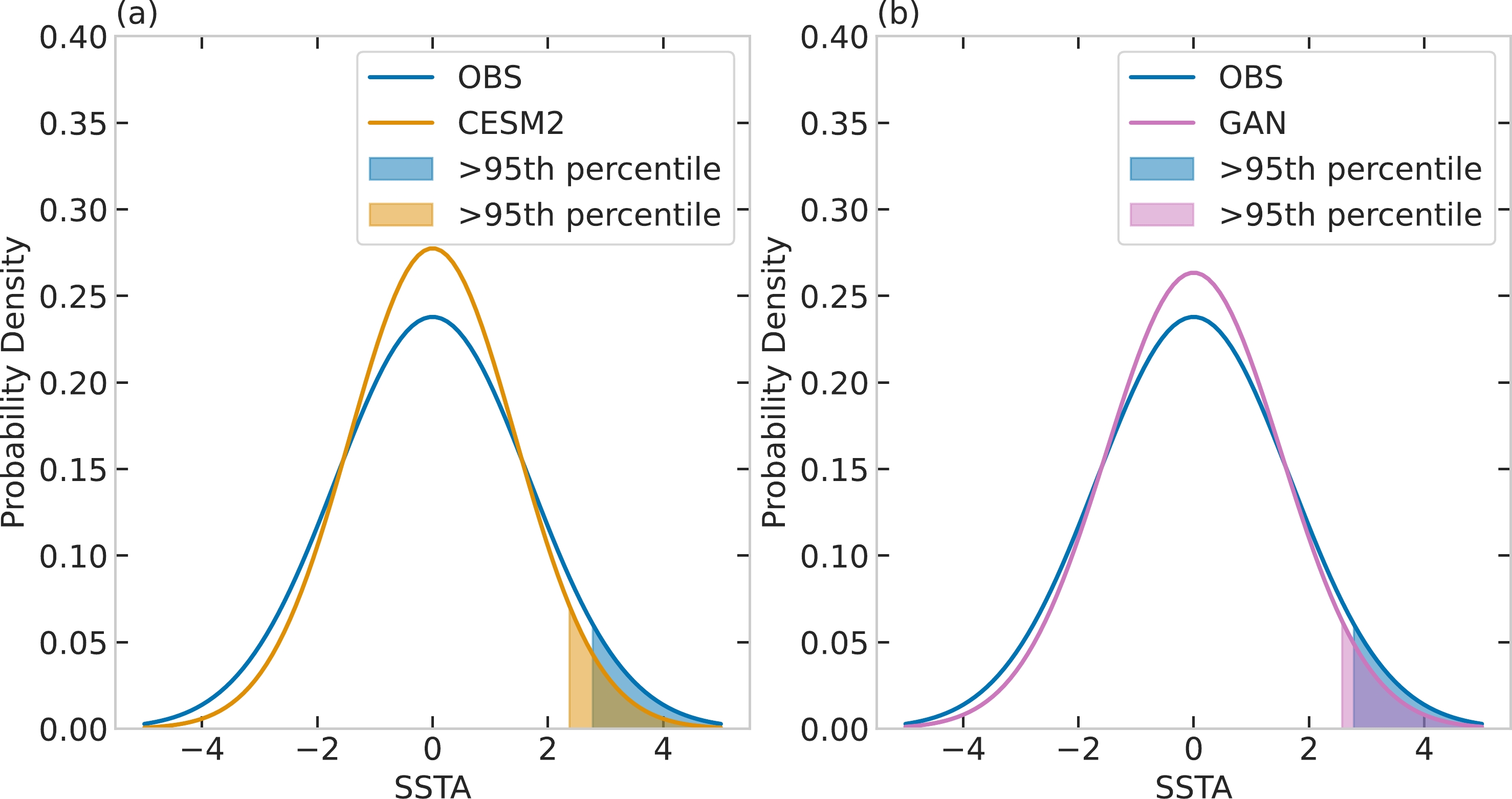
Particularly noteworthy is the significant reduction of the overestimation bias in the central and eastern tropical Pacific and the enhancement in the underestimation in the northeast Pacific, making CycleGAN's results more consistent with NCEP. Figures 8 and 9 present probability density functions (PDFs) of SSTAs in the tropical (5°S–5°N) and northeast (40°–60°N; 180°–120°W) Pacific, respectively. On average, CESM2 exhibits a wider distribution in the tropics, indicating a stronger variability. CESM2 has a 95th percentile of 1.41 degrees for the tropical region, while NCEP only has 1.18 degrees, resulting in a 19.5% overestimation. This aligns with the earlier result of the overestimation of SSTAs in the tropical region, especially in the central and eastern Pacific (Fig. 7). After correction, the distribution of SSTA in the tropics closely matches observations, with 95th percentiles of approximately 1.17, indicating a substantial reduction in the overestimation bias of CESM2 in the tropics. A similar situation is observed in the northeast Pacific. In this area, the SSTA distribution in CESM2 is overall narrower than observations, indicating a lower variability. Correspondingly, its 95th percentile is lower than that of NCEP. After correction, the distribution and the 95th percentile of SSTAs are much closer to NCEP.

Figure 8.  PDFs of average tropical SSTAs for (a) NCEP and CESM2, and (b) NCEP and CycleGAN. Shading indicates areas where the SSTA is above the 90th percentile.

Figure 9.  Same as in Fig. 8, but for the Northeast Pacific SSTAs.

Unlike methods such as modified QM that directly adjust data by quantiles to make the local distribution closer to observations, the CycleGAN learns and transforms high-dimensional data features. An important question naturally arises: which key processes does CycleGAN capture that result in the improvement of simulated SST extremes? To address this question, we further perform an analysis of variability at various timescales, involving interannual variabilities and frequencies that less than 90 days (encompassing the Madden−Julian Oscillation (MJO), Intraseasonal Oscillation (ISO), and synoptic-scale eddies). Figure 10a presents the interannual standard deviation of DJF SSTs based on observations. It primarily exhibits an ENSO-like pattern in the equatorial central and eastern Pacific. Moreover, notable high-variability regions are evident in the Northeast Pacific, North Pacific, mid-latitudes in the South Pacific, and adjacent to western boundary currents. In general, the spatial distribution of SST interannual variability in observations closely resembles the distribution of the 95th percentile of SSTA (shown in Fig. 7), indicating the direct influence of interannual variability, especially ENSO, on extreme SSTs as in previous studies (Doi et al., 2015; Oliver et al., 2021). Additionally, ENSO can induce SST variations in the Northeast Pacific and North Atlantic regions by exciting Rossby wave trains (Wang et al., 2021, 2022, 2023), further influencing extreme events in those areas (Trenberth et al., 1998; Johnson and Kosaka, 2016). When compared to observations, CESM2 exhibits an overall overestimation of interannual variability, particularly pronounced in the central-eastern Pacific. This overestimation is likely related to the higher ENSO variability within CESM2 (Capotondi et al., 2020). The consistency of the stronger interannual variability in the tropical central-eastern Pacific and the larger bias of extreme SSTAs in Fig. 7 suggest that the overestimation of interannual variability is a key factor contributing to the high bias in extremes in CESM2. In contrast to CESM2, SST fields corrected by the CycleGAN show a substantial reduction in the error in interannual variability, with the RMSE decreasing from 0.31 to 0.1. CycleGAN-corrected results exhibit a closer match to observations in terms of intensity, particularly in the tropical Pacific, South Pacific, Atlantic, and Indian Ocean. While the intensity in the tropical central-eastern Pacific remains higher than observed, notable improvements are observed compared to CESM2, consistent with the enhancement seen in the extreme SSTAs for this region in Fig. 7. Concerning intraseasonal and synoptic-scale variability, the variability in NCEP is predominantly concentrated in the tropical Pacific and western boundary current regions (Fig. 10d), likely associated with boundary currents, subseseanal variations (Liu et al., 2022a, 2022b), and active mesoscale eddy activity (Oliver et al., 2021). CESM2 simulations generally underestimate variability at these scales (Fig. 10e). In contrast, CycleGAN-corrected SSTs exhibit substantial improvements, especially in the Northeast Pacific, where the distribution is in closer agreement with NCEP (Fig. 10f). In summary, the CycleGAN demonstrates significant improvements in SST variability at different timescales, facilitating more accurate simulation of the complex oceanic dynamic processes, particularly regarding interannual variability and variability at intraseasonal and synoptic scales.

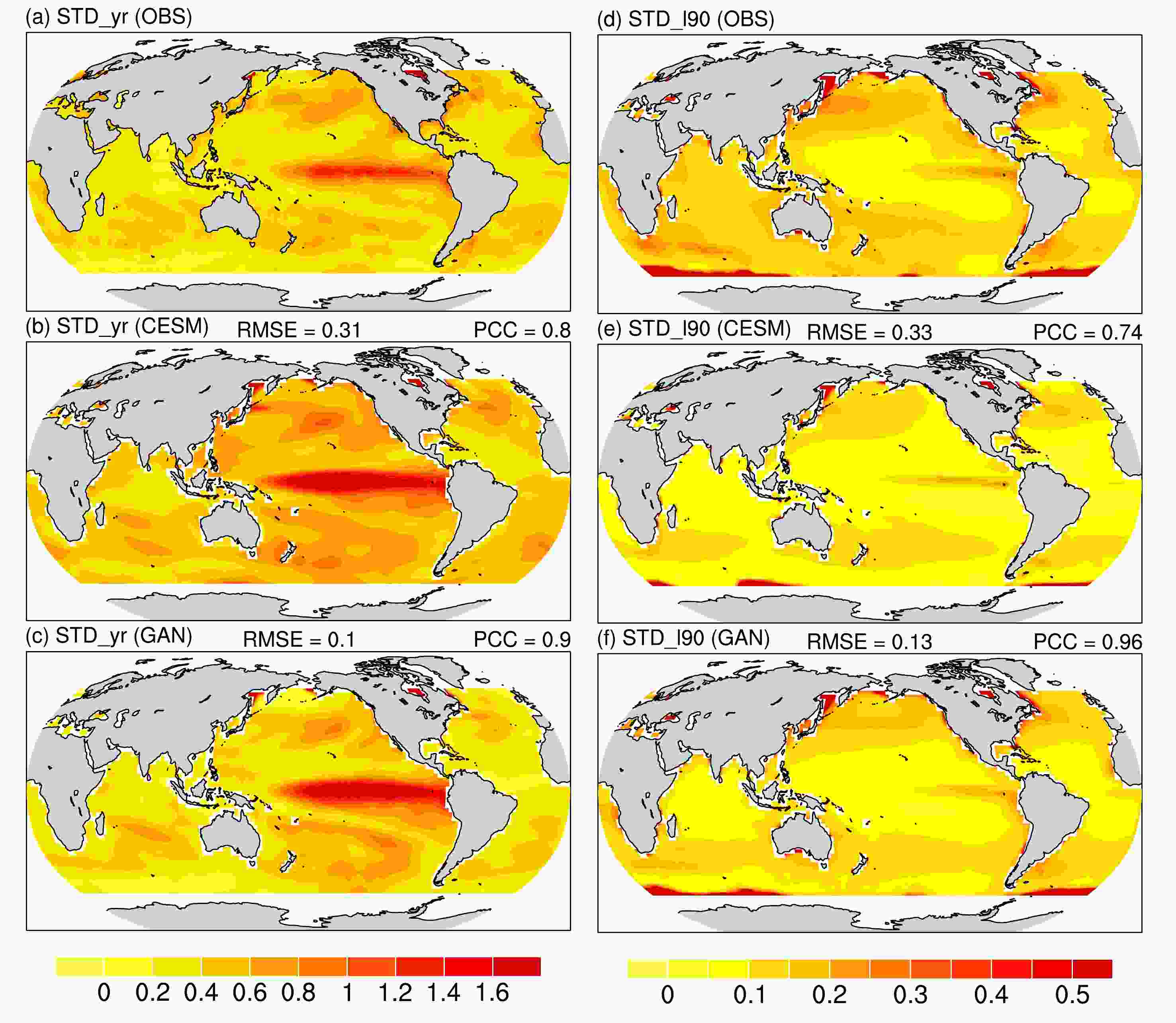
Figure 10.  Standard deviations of (left) interannual DJF SSTAs and (right) SSTAs filtered by a band of 2–90 days in (a, d) NCEP, (b, e) CESM2, and (c, f) CycleGAN, respectively.

In this study, we employed CycleGAN to correct the daily SSTs from CESM2 historical simulations. We conducted a comprehensive assessment of this model, considering various aspects such as climatology, interannual variability, and extremes. Our findings reveal significant improvements across these evaluation dimensions. At the climatological scale, the CycleGAN substantially reduced bias in annual mean climatological SST. Specifically, there is a 58% reduction in RMSE relative to CESM2, from 1.25 (1.19–1.28) degrees in CESM2 to 0.52 (0.4–0.57) degrees. At the interannual scale, involving two primary tropical modes, ENSO and IOD, we observe significant enhancements in simulating these modes with the CycleGAN. For ENSO SSTAs, the RMSE decreases from 0.14 to 0.06, corresponding to a reduction of 57%. CycleGAN effectively addresses a common bias of ENSO SST found in many climate models, known as the excessive westward bias in the equatorial Pacific that traditional methods, like quantile mapping, struggle to rectify. In the case of IOD, CESM2 tends to produce excessively strong and westward-extending anomalies in the southeastern Indian Ocean. After the correction, these biases are substantially reduced, resulting in an increased PCC of up to 0.92.

Moreover, we investigate the performance in simulating SST extremes. The CycleGAN corrects the overestimation in extremes in most regions and addresses the underestimation in the Northeast Pacific. The improved performance of the CycleGAN in simulating the distribution of SSTAs and their associated extremes can be attributed to its ability to capture different temporal scales of variability, including interannual variability and variability at intraseasonal and synoptic scales, encompassing periods shorter than 90 days.

In summary, our study demonstrates that the CycleGAN offers comprehensive enhancements across various timescales and physical processes. Its utility extends beyond merely correcting specific statistical measures such as first and second-order moments locally; it also enhances the simulation of critical air-sea coupling modes like ENSO and IOD. These findings underscore the significant potential of CycleGAN as a valuable tool for climate model correction and climate projection.

We employ NCEP data for the evaluation of SST extremes. It is crucial to highlight the potential inconsistency among various observational datasets at the daily timescale, particularly in oceanic data. Consequently, it is essential to clarify that the presented results regarding SST extremes should be interpreted as an assessment of the capacity of CycleGAN to enhance the simulation of SST extremes rather than its precision in replicating observations. Achieving the latter would demand a more extensive dataset, particularly observational station data.

Moreover, it is crucial to acknowledge that, beyond the correction of historical simulations, the central consideration is the adaptability of these methods to future projections. Recent studies, exemplified by Hess et al. (2022), suggest that CycleGAN, through post-processing or incorporating constraints like global mean values, can reproduce trend signals under global warming. Further research is needed to refine the capability of capturing regional-scale warming responses. Subsequent investigations should also involve the development of correction datasets encompassing multiple models and variables, accompanied by a comprehensive analysis of physical mechanisms and laws in the corrected data. Comparisons with methods integrated with climate models, such as surface flux adjustments, should be explored. Furthermore, the direct coupling of the proposed correction method with climate models represents a critical avenue for future inquiry.

Acknowledgements. The study is jointly supported by the National Natural Science Foundation of China (Grant Nos. 42141019 and 42261144687), the Second Tibetan Plateau Scientific Expedition and Research (STEP) program (Grant No. 2019QZKK0102), the Strategic Priority Research Program of the Chinese Academy of Sciences (Grant No. XDB42010404), the National Natural Science Foundation of China (Grant No. 42175049) and the Guangdong Meteorological Service Science and Technology Research Project (Grant No. GRMC2021M01). Ya WANG would like to thank the National Key Scientific and Technological Infrastructure project “Earth System Science Numerical Simulator Facility” (EarthLab) for computational support and Prof. Shiming XIANG for many useful discussions. Niklas BOERS acknowledges funding from the Volkswagen foundation. The code of CycleGAN can be found in https://github.com/junyanz/CycleGAN.