


 DownLoad:


-
One of the important processes for cloud formation and development is water vapor condensation. The evolution of the cloud droplet spectrum (CDS) during condensation highly impacts the other microphysical processes, such as the formation of rain, the nucleation of ice, and so on (Milbrandt and Yau, 2005a; Petters et al., 2006; Milbrandt et al., 2021). The numerical simulation for the condensational growth of a population of cloud droplets remains a challenge (Khain et al., 2015).
The evolution of the CDS can be described by the two mathematical approaches. The first is by bin schemes in which the number concentration in each bin is determined individually for all microphysical processes (Tzivion et al., 1994; Khain et al., 2000). Another method is by bulk parameterization microphysics schemes in which the size distribution is prescribed to fit a function form (e.g., a gamma distribution), and the parameters vary according to changes in prognostic moments. In most bulk parameterization schemes, the CDS is expressed by a Gamma distribution function with three parameters, the intercept parameter, the shape parameter, and the slope parameter. The bulk parameterization schemes can be classified into three kinds of schemes by the number of parameters considered: single-moment schemes, double-moment schemes, and triple-moment schemes.
The hydrometeor mass mixing ratio is predicted, and the slope parameter is diagnosed in single-moment schemes (Kessler, 1969; Lin et al., 1983; Cotton et al., 1986; Tao and Simpson, 1993; Kong and Yau, 1997; Bae et al., 2018). In double-moment schemes, the intercept parameter and slope parameter are diagnosed by the number concentration and the mass mixing ratio (Ziegler, 1985; Levkov et al., 1992; Harrington et al., 1995; Cohard and Pinty, 2000; Seifert and Beheng, 2001; Morrison et al., 2009). However, the shape parameter is either fixed or diagnosed by empirical formulas without adding a new degree of freedom (Milbrandt and Yau, 2005a; Morrison and Grabowski, 2007; Xie et al., 2013, 2017).
For the double-moment schemes with a constant shape parameter, the simulated cloud spectra for pseudo-adiabatically ascending cloud parcels may not obey their condensational growth behavior. If there are not the new cloud droplets from nucleation, the breadths of the spectra will become narrower and narrower because the growth rates of smaller droplets are higher than those of bigger ones (Rogers and Yau, 1989). A constant shape parameter may result in the steady breadth of the droplet spectrum. It is evident that the CDS is spuriously broadened in the simulations by the current double-moment condensation schemes with fixed shape parameters (Zhang, 2015; Deng et al., 2018). Such a phenomenon has also been found in the spectrum evolution of ice crystals during depositional growth with a double-moment scheme (Chen and Tsai, 2016). Shape parameters diagnosed by empirical formulas can improve the spectrum evolution (Milbrandt and Yau, 2006), but the empirical formulas lack universality (Loftus et al., 2014).
However, the shape parameter is very important. It can describe the relative dispersion of the distribution for the hydrometeors and thus affect the cloud’s optical properties and precipitation (Liu and Daum, 2000; Milbrandt and Yau, 2005a). It is also related to the first indirect effect of aerosols (Liu and Daum, 2002; Xie et al., 2017) and the second indirect effect of aerosols (Liu and Daum, 2004; Xie and Liu, 2011; Xie et al., 2013). Recent studies have paid much attention to the influence of the shape parameter on cloud microphysical processes (Milbrandt and Yau, 2005a, b, 2006; Loftus et al., 2014; Naumann and Seifert, 2016). But Khain et al. (2015) pointed out that the current, state-of-the-art three-parameter schemes were mainly used to simulate raindrops with large terminal velocities. Milbrandt and Yau (2005b) applied the reflectivity factor to diagnose the shape parameter, where the change rate of the reflectivity factor was obtained by the change rate of the mass mixing ratio and the number concentration. Still, the shape parameter remains unchanged in the scheme during condensation. In fact, studies concerning the influence of the shape parameter on the evolution of the CDS during condensation have still not been well addressed. Therefore, with the improvement of computing capabilities, it is desirable to diagnose the shape parameter by adding a new degree of freedom and accurately simulate the spectrum evolution of cloud droplets during condensation.
In this study, the influence of the shape parameter on condensational growth, and the spectrum evolution of cloud droplets were studied based on the shape parameter diagnosed by the combination of the number concentration, the water content and the reflectivity factor. We find that the new scheme greatly improves upon the accuracy of the CDS compared to the double-moment schemes.
The remainder of this paper is organized as follows. The mathematical methods are introduced in section 2. Theoretical validations of the new scheme are given in section 3, and our conclusions are given in section 4.
-
The Gamma size distribution function used to describe the size distribution of hydrometeors has the following form:
where m is the mass of a single cloud droplet,
$ f(m) $ is the number density of the cloud droplets with mass m,$ \alpha $ is the shape parameter,$ \beta $ is the slope parameter and$ {N}_{0} $ is the intercept parameter.The double-moment schemes apply two moments, representing the number concentration (
$ {N}_{\mathrm{c}} $ ) and the cloud water content ($ {q}_{\mathrm{c}} $ ). With Eq. (1), the analytical solutions of the number concentration and the cloud water content can be derived as follows:The slope parameter and intercept parameter can be obtained by the combination of Eqs. (2) and (3):
The above equations are used to diagnose the slope and intercept parameters in the bulk double-moment scheme with a fixed shape parameter. Still, there are other double-moment schemes in which the shape parameters are also diagnosed by empirical formulas, so we chose the method of Morrison and Grabowski (2007) (hereafter MG), given the simulations of spectra and moments of the mass distribution.
In the MG scheme, the shape parameter is diagnosed by the number concentration of cloud droplets as follows (Morrison and Grabowski, 2007):
To facilitate comparison with the new scheme, the spectrum distribution is expressed by Eq. (1).
The mass condensation growth rate of a single cloud droplet can be given as:
where s represents the ambient supersaturation,
$ {\rho }_{\mathrm{w}} $ is the density of water, and$ \xi $ is related to the vapor diffusion and the latent heat release, as given by Eq. (8):Here
$ {R}_{\mathrm{v}} $ is the individual gas constant for water vapor, T represents the ambient temperature, L(T) is the latent heat,$ {K}_{\mathrm{a}} $ is the coefficient of thermal conductivity of air,$ {e}_{\mathrm{w}} $ is the saturation vapor pressure, and$ {D}_{\mathrm{v}} $ represents the molecular diffusion coefficient.The change rate of cloud water content (
$ {q}_{\mathrm{c}} $ ) during condensation can be obtained by the combination of Eqs. (1), (3), and (7):The research reveals that the empirical formulas like Eq. (9) lack universality (Loftus et al., 2014). So based on another part of our research, the diagnosis equation of shape parameter is obtained by introducing a reflectivity factor in the new scheme. The reflectivity factor (
$ {Z}_{\mathrm{c}} $ ) can be calculated by its definition (proportional to the second moment of the mass distribution) and through Eq. (1):Based on previous research (Yang and Yau, 2008; Chen and Tsai, 2016), the change rate of
$ {Z}_{\mathrm{c}} $ during condensation can be obtained by the combination of Eqs. (1), (7), and (10):The shape parameter and the slope parameter can be calculated by the combination of Eqs. (2), (3), and (10):
The above parameterization schemes will be tested in a parcel model with constant supersaturation values and a 1.5D Eulerian model with the real sounding profile of Rain in Shallow Cumulus over the Ocean (RICO) (Rauber et al., 2007; Wang et al., 2016). The 1.5D model consists of two cylinders. The updraft area is located in the inner cylinder, and the downdraft area is the space between the inner and outer cylinders. The exchanges of cloud droplets and aerosols due to the entrainment and detrainment between the cloud and environment are described by the continuity equation. The details of the model were introduced in the paper of Sun et al. (2012a).
-
To verify the advantages and disadvantages of the new parameterization scheme, the analytical solution of the CDS evolution is calculated based on Rogers and Yau (1989) as follows:
Or
where
$ {f}_{m}(m,t) $ is the distribution of cloud droplets with mass$ m $ at time$ t $ .Since
where
$ {f}_{\mathrm{l}\mathrm{n}\left(m\right)}(m,t) $ is the distribution of cloud droplets with logarithmic mass$ \mathrm{l}\mathrm{n}\left(m\right) $ at time$ t $ .So the change rate of the CDS with logarithmic mass based on the Lagrangian view can be given during condensation as follows:
upon substituting Eq. (7) into Eq. (17), we obtain:
and integrating Eq. (18) from
$ {t}_{0} $ to$ {t}_{0}+\Delta t $ yields:We further discretized the CDS into 3000 mass bins with the following relationship:
where
$ m\left(i\right) $ represents the mass of cloud droplets in the i-th mass bin.If the influences of solution and curvature on droplet equilibrium vapor pressure are ignored, the radius of the cloud droplet in each bin can be obtained analytically:
where
$ r\left(i,j\right) $ is the cloud droplet radius of the i-th mass bin at the time step$ j $ .At the same time, if only condensation is taken into account for the microphysical processes of droplets, the number concentration of cloud droplets in each bin is conserved in the Lagrangian view:
and the analytical cloud water content (
$ {q}_{\mathrm{c}} $ ) and volume-mean radius ($ {r}_{\mathrm{c}\_\mathrm{v}} $ ) per moment can also be obtained:where
$ {r}_{\mathrm{c}\_v} $ is in centimeters. -
An obvious monotonic relationship exists between the shape parameter and the volume-mean radius based on the simulation of the Lagrangian analytical solution based on Case 1 in Table 1, so the fitting function for the relationship between the shape parameter and the volume-mean radius with a correlation coefficient of 0.99 is obtained to modify the double-moment scheme as follows:
Cases $ s $ $ {N}_{\mathrm{c}} $ (cm–3) $ {q}_{\mathrm{c}} $ (g cm–3) $ {Z}_{\mathrm{c}} $ (cm6 cm–3) $ \alpha $ $ \beta $ (g–1) Case 1 0.1% 150 7.5 × 10⁻⁷ 2.05 × 10⁻¹⁴ 2 4 × 10⁸ Case 2 0.3% 150 7.5 × 10⁻⁷ 2.05 × 10⁻¹⁴ 2 4 × 10⁸ Case 3 0.03% 150 7.5 × 10⁻⁹ 1.82 × 10⁻¹⁸ 3 6 × 10¹⁰ Case 4 0.01% 150 7.5 × 10⁻⁹ 1.82 × 10⁻¹⁸ 3 6 × 10¹⁰ Table 1. The initial conditions.
In the modified double-moment scheme, the shape parameter can be calculated by Eq. (25), while the slope and intercept parameters are still obtained by Eqs. (4) and (5).
-
The time evolution of the CDS was simulated under a simplified scenario of a constant supersaturation at T = 283 K and P = 80 000 Pa. To show the importance of the shape parameter on the evolution of the CDS, the simulation comparisons between the double-moment scheme, which uses Eqs. (4) and (5) to determine the slope and intercept parameters with a fixed shape parameter (hereafter DM), the modified DM (DM-modified), MG, and the new triple-moment schemes (hereafter TM) were performed. Equations (4), (5), and (6) were adopted to determine the slope, intercept, and shape parameters in the MG simulations and Eqs. (4), (5), and (25) were used to determine the slope, intercept, and shape parameters in the DM-modified simulations. Equations (12), (13), and (5) were applied to calculate the shape, slope, and intercept parameters in the TM scheme.
All differential equations were resolved through a sixth-order Runge-Kutta algorithm. The analytical solution, based on the Lagrangian bin scheme (hereafter LBS), is introduced as a comparison criterion. By comparing to the LBS, we can characterize the advantages and disadvantages of different bulk parameterization schemes in the simulation of the CDS during condensation. We chose four idealized warm rain formation cases, shown in Table 1. The initial shape parameters of those schemes are shown in Table 1.
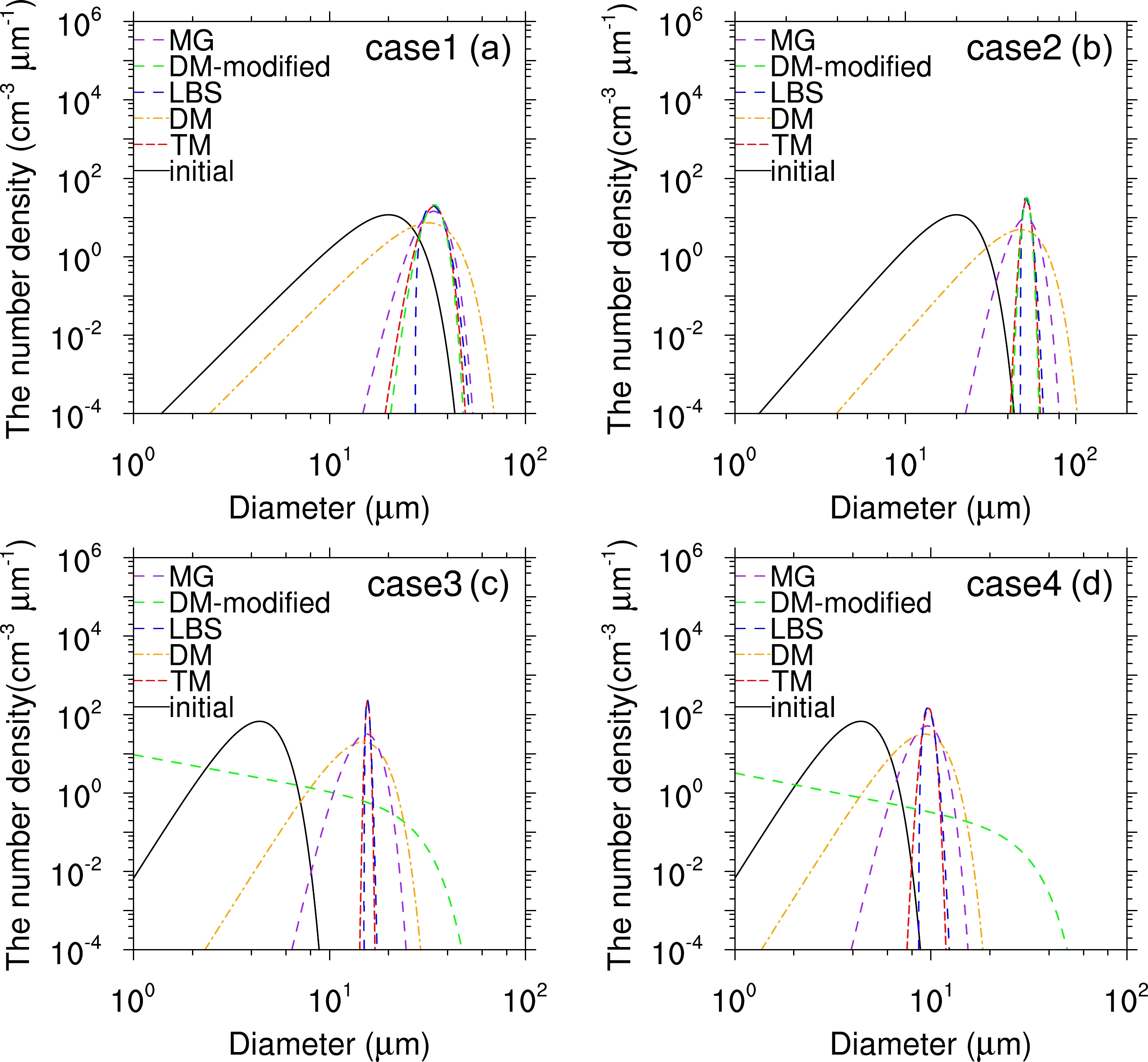
The evolution of the simulated CDS with the LBS shows that the CDS becomes narrower and narrower since the growth rates of the cloud droplets are inversely proportional to their radii, where the small droplets grow more quickly than the large droplets (Fig. 1). Figure 1 also illustrates that the CDS simulated with the DM scheme is spuriously broadened. The assumption of a constant shape parameter ultimately results in the spectrum of a pseudoadiabatic ascending cloud parcel not obeying the condensation growth behavior. Therefore, the DM scheme cannot adequately describe the evolution of the CDS during condensation. Furthermore, the broadening of the right tail of the CDS in the DM scheme indicates that the number concentration of the large cloud droplets is overestimated. This overestimation may accelerate warm rain formation. The spectra simulated with the DM-modified scheme are close to those of the LBS in Case 1 and Case 2 in Table 1, but they are spuriously broadened in Case 3 and Case 4 in Table 1. This is because the volume-mean radii are small, so the shape parameter values are close to 0 in Cases 3 and 4. If the lower-level cut-off value of the shape parameter in Eq. (25) is set to 2, the results for the DM-modified scheme would be improved for Case 3 and Case 4. In general, the fitting function of the shape parameter in the DM-modified scheme has limitations. A shape parameter diagnosed by the number concentration improves the evolution of the CDS in the MG scheme, but the CDS simulated by the MG scheme is still wider than that with the LBS. In the MG scheme, the shape parameter remains unchanged after the second time step due to the constant number concentration of cloud droplets during condensation. The evolution of the CDS simulated by the TM scheme is consistent with that of the LBS, but the small droplets on the left tail of the CDS simulated by the TM scheme grow slower than those simulated by the LBS with a supersaturation value of 0.1% in Case 1 (Fig. 1a). The difference between the TM scheme and the LBS in their respective CDS simulations becomes small under a supersaturation value of 0.3% (Fig. 1b). So the errors decrease with increasing supersaturation values. The shape parameter of the TM scheme is numerically diagnosed by the combination of the number concentration, the cloud water content, and the reflectivity factor [see Eq. (12)]. Such a treatment ensures accurate calculations of the shape parameter and the CDS. The shape parameter will be analyzed later. The key point of these experiments is that the shape parameter plays an important role in the evolution of the CDS and the condensation growth of a population of cloud droplets.
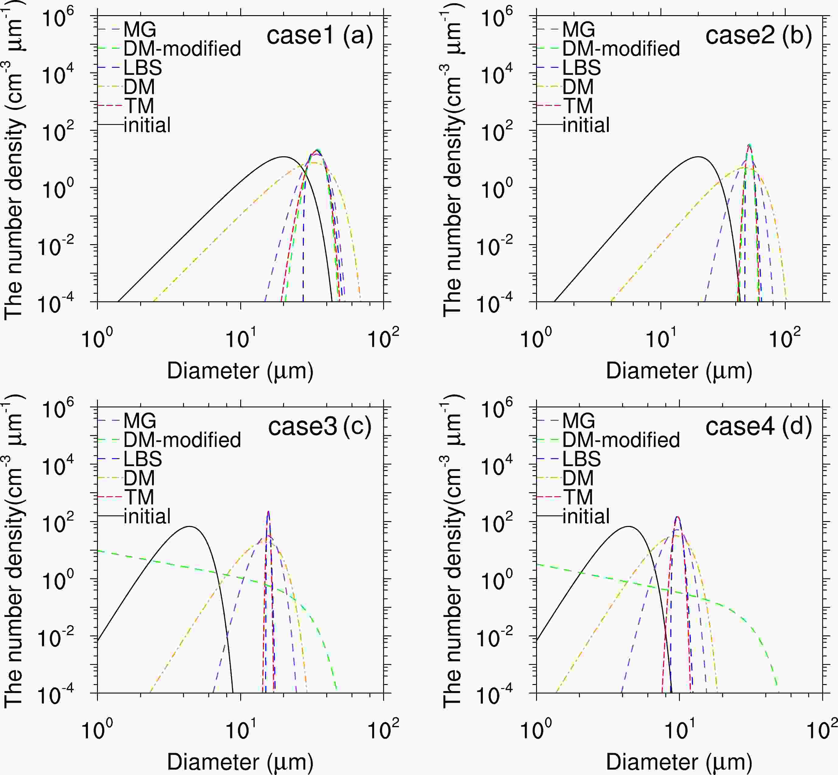
Figure 1. Cloud droplet spectra simulated with different condensation schemes, ignoring the solution and curvature effects at 10 min. for (a) Case 1; (b) Case 2; (c) Case 3; (d) Case 4. The blue dashed lines denote the cloud droplet spectra simulated with the Lagrangian bin scheme (LBS), the orange dotted lines represent the cloud droplet spectra simulated with the double-moment scheme (DM), the green dashed lines are the cloud droplet spectra simulated with the modified DM scheme (DM-modified), the purple dashed lines represent the cloud droplet spectra simulated with the Morrison and Grabowski (2007) scheme (MG), and the dashed red lines denote the cloud droplet spectra with the new scheme (TM).
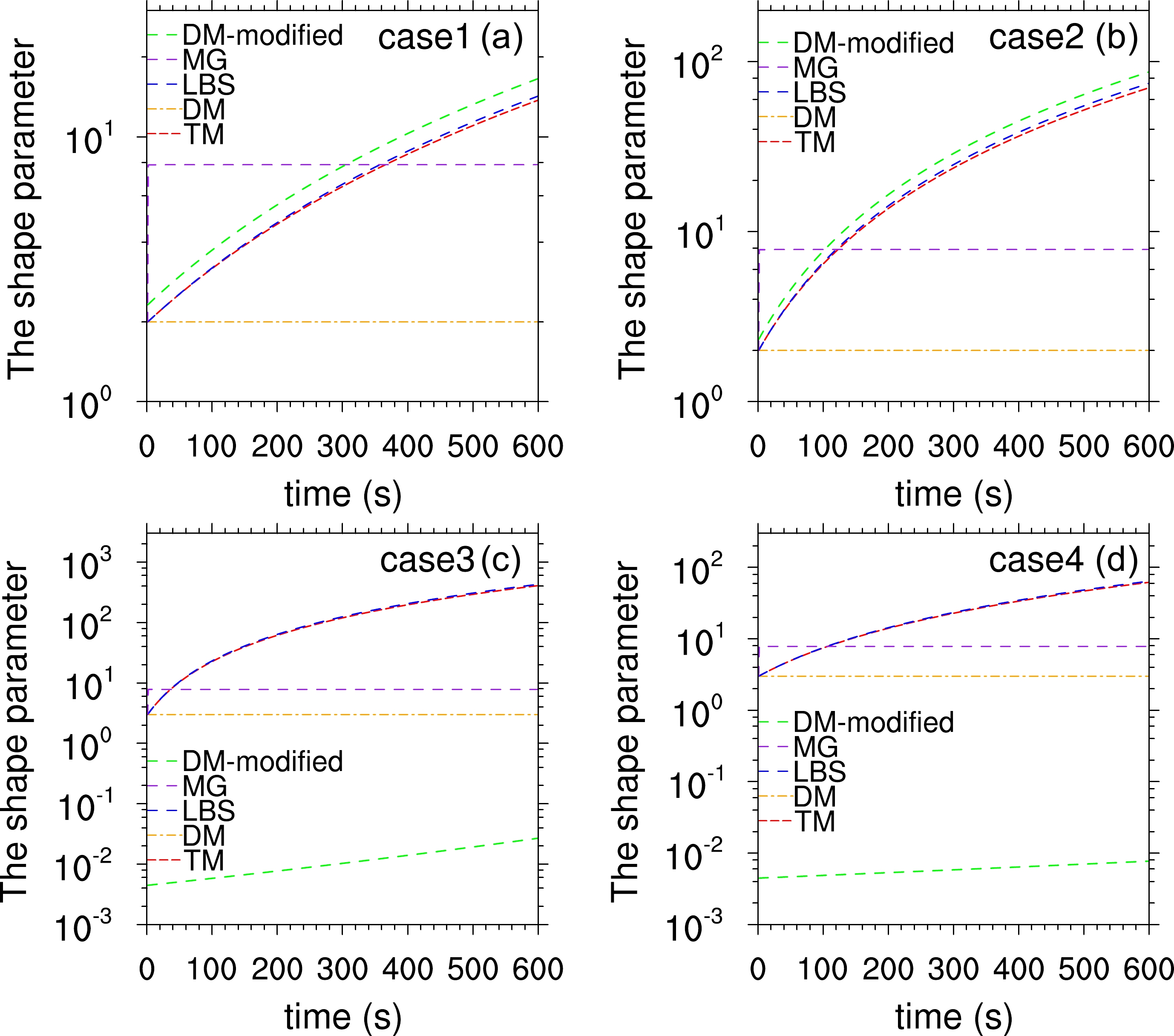
Figure 2 shows the evolution of the shape parameters simulated with the LBS and the TM, DM, DM-modified, and MG schemes. Although there is no shape parameter in the LBS, the shape parameter can be calculated using the reflectivity factor, the cloud water content, and the number concentration by Eq. (12). Therefore, we assumed that the size distribution could be fitted by a Gamma distribution function and the shape parameter of the LBS was given as a comparison criterion. On the contrary, the shape parameters of the DM scheme are constant. The MG scheme diagnostic is based on the number concentration of cloud droplets, and the number concentration of cloud droplets is constant in idealized condensation simulations. Therefore, the shape parameters in the MG scheme are diagnosed at the second time step and remain unchanged afterward. The shape parameters of the DM-modified scheme are variable and close to those of the LBS in Case 1 and Case 2, but they are much smaller than those of the LBS in Case 3 and Case 4. The evolution of the shape parameters in the simulations in the TM scheme match those of the LBS well, but the shape parameters in the TM scheme are slightly lower than those of the LBS in Case 1 and Case 2 (Figs. 2a and 2b). The differences in the shape parameters of large values may result in small differences in spectrum widths, which are inversely proportional to the shape parameters, as shown in Figs. 1a and 1b, and vice versa. In general, the shape parameters of the TM scheme are close to those of the LBS. It can be found that such flexibility of the shape parameter in the new condensation scheme ensures an accurate description of the CDS.
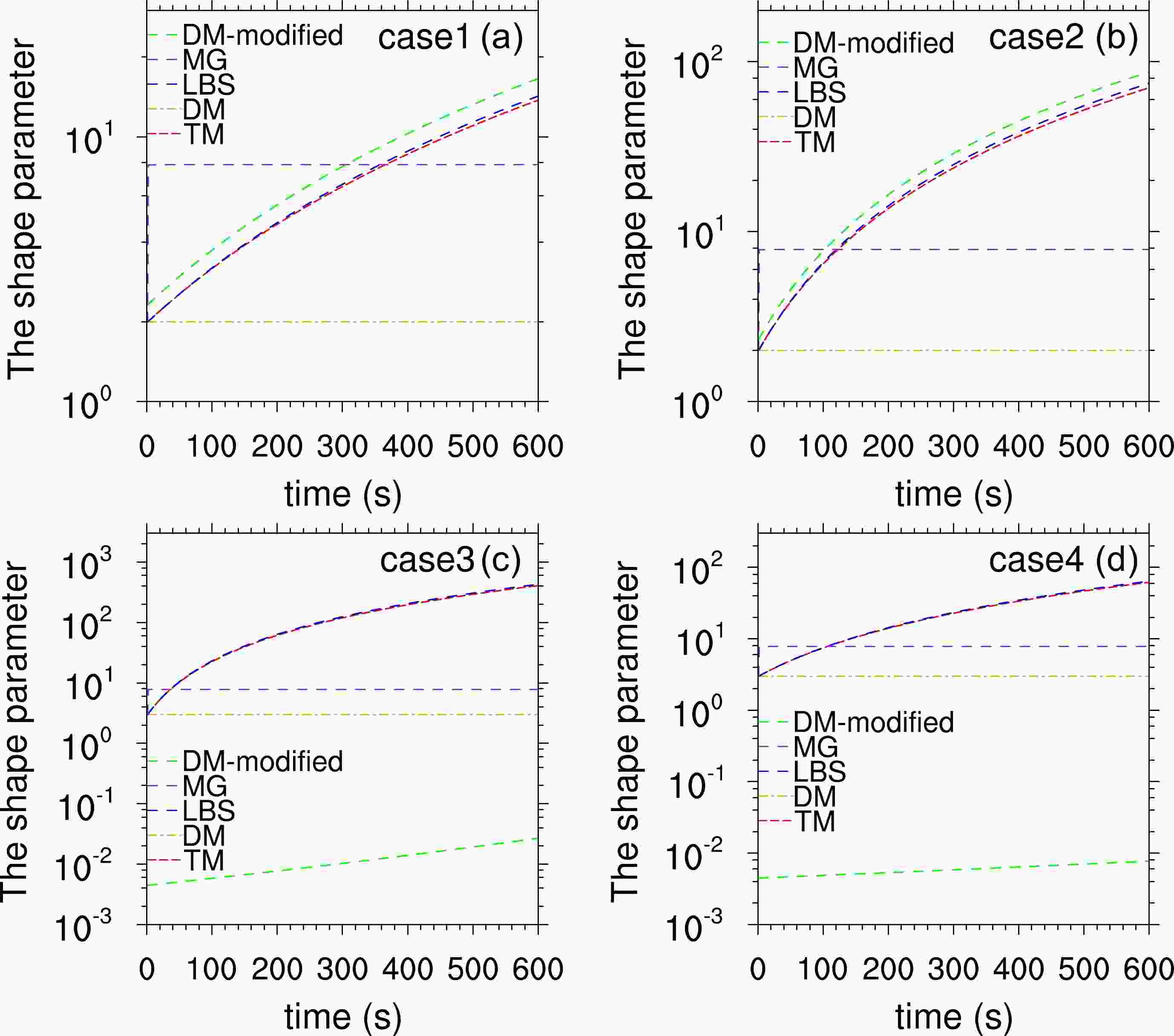
Figure 2. Evolution of the shape parameters simulated with the LBS and TM, DM, DM-modified, and MG schemes in (a) Case 1; (b) Case 2; (c) Case 3; (d) Case 4.
-
Figures 3 and 4 show the evolution of
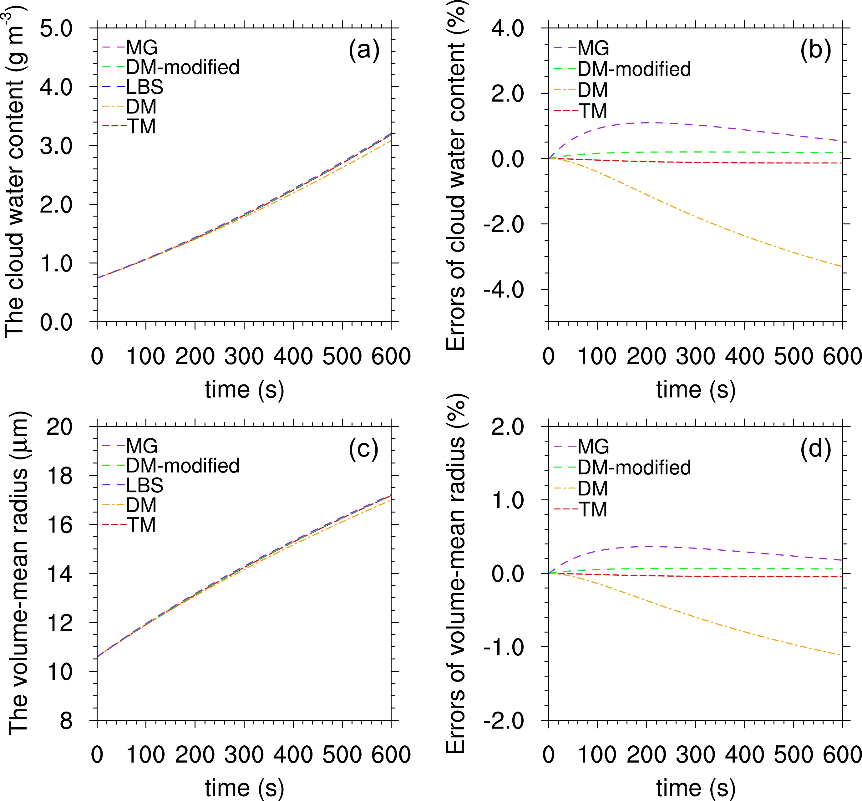
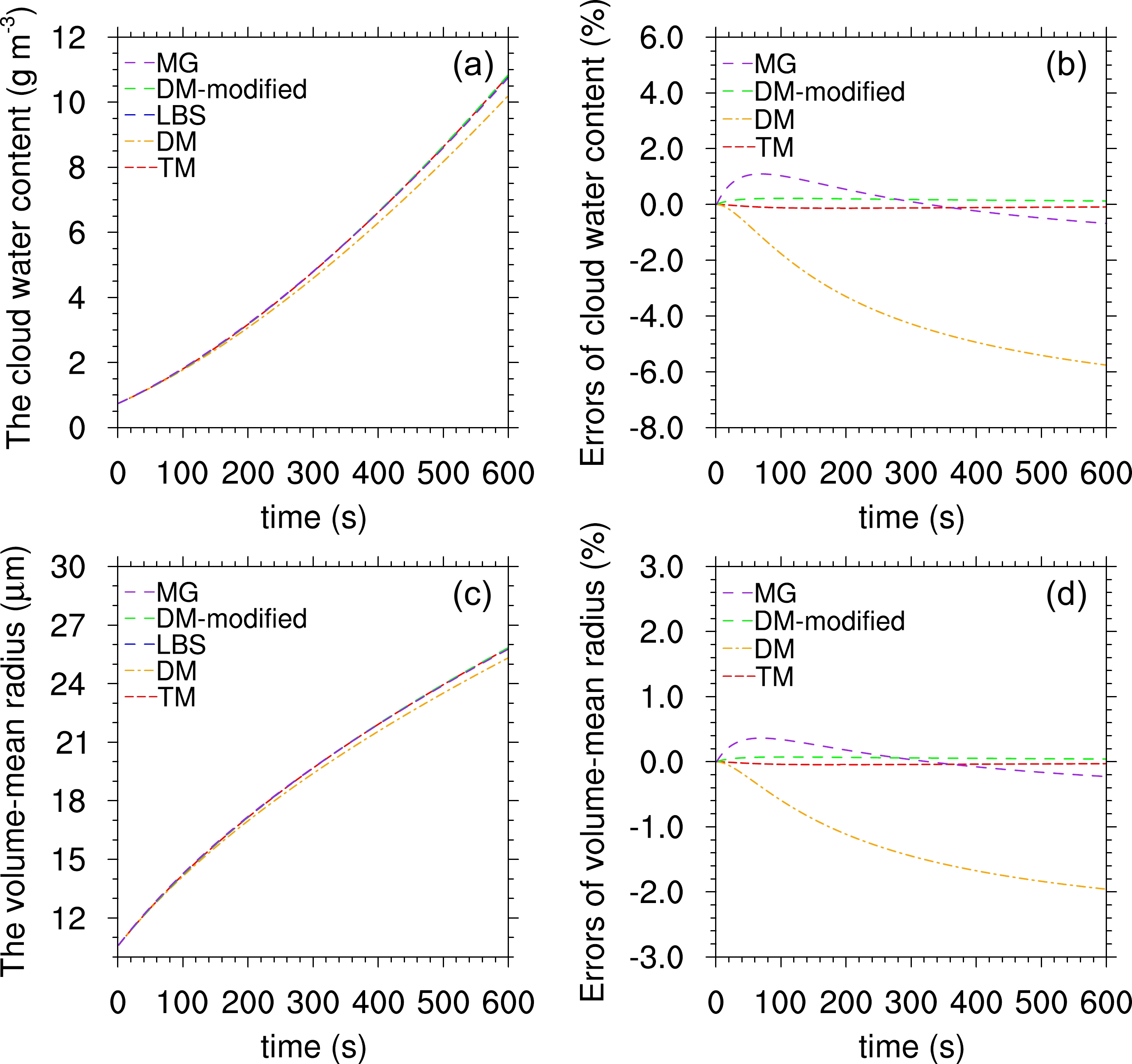
$ {q}_{\mathrm{c}} $ and$ {r}_{\mathrm{c}\_\mathrm{v}}, $ in the LBS and TM, DM, DM-modified, and MG schemes for Case 1 and Case 2. Figure 3 indicates that the DM scheme underestimates$ {q}_{\mathrm{c}} $ and$ {r}_{\mathrm{c}\_\mathrm{v}} $ . The errors relative to the analytical solutions reach −3.3% and −1.5%, with a supersaturation value of 0.1%. The errors increase with time and supersaturation. The maximum errors in$ {q}_{\mathrm{c}} $ and$ {r}_{\mathrm{c}\_\mathrm{v}} $ simulated with the DM scheme can reach −5.8% and −2.0% with a supersaturation value of 0.3%, as shown in Fig. 4. The MG scheme overestimates$ {q}_{\mathrm{c}} $ and$ {r}_{\mathrm{c}\_\mathrm{v}} $ before 300 s under a supersaturation of 0.1% and 0.3% and underestimates$ {q}_{\mathrm{c}} $ and$ {r}_{\mathrm{c}\_\mathrm{v}} $ after 300 s with a supersaturation of 0.3%; the errors of underestimations increase with time. In general,$ {q}_{\mathrm{c}} $ and$ {r}_{\mathrm{c}\_\mathrm{v}} $ , simulated with MG scheme, are close to those of the LBS. The DM-modified and TM schemes lead to small and steady errors for both the evolution of$ {q}_{\mathrm{c}} $ and$ {r}_{\mathrm{c}\_\mathrm{v}} $ . The maximum errors in the evolution of$ {q}_{\mathrm{c}} $ and$ {r}_{\mathrm{c}\_\mathrm{v}}, $ simulated by TM, are all less than 0.2%, respectively (Figs. 3b, 3d, 4b, and 4d). The evolutionary characteristics of$ {q}_{\mathrm{c}} $ and$ {r}_{\mathrm{c}\_\mathrm{v}} $ in the LBS and TM, DM, and MG schemes for Case 3 and Case 4 are similar to those of Case 1 and Case 2, but the simulations of$ {q}_{\mathrm{c}} $ and$ {r}_{\mathrm{c}\_\mathrm{v}} $ in the DM-modified scheme have large errors, as shown in Fig. 5.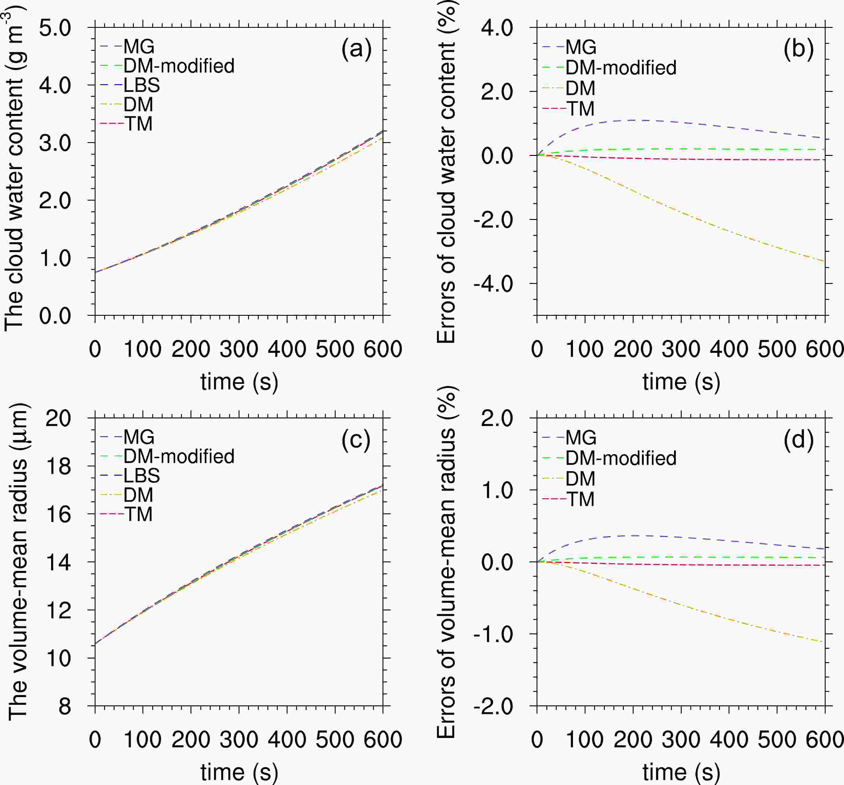
Figure 3. The evolution of the cloud water content (
$ {q}_{\mathrm{c}} $ ) and the volume-mean radius ($ {r}_{\mathrm{c}\_\mathrm{v}} $ ) with different schemes: the LBS and DM, DM-modified, MG, and TM schemes, and the errors of DM, DM-modified, MG, and TM schemes compared with the LBS under the supersaturation value of 0.1% in Case 1. (a) The evolution of the cloud water content ($ {q}_{\mathrm{c}} $ ); (b) the errors of the cloud water content ($ {q}_{\mathrm{c}} $ ) for the DM, DM-modified, MG, and TM schemes; (c) the evolution of the volume-mean radius ($ {r}_{\mathrm{c}\_\mathrm{v}} $ ); (d) the errors of the volume-mean radius ($ {r}_{\mathrm{c}\_\mathrm{v}} $ ) for DM, DM-modified, MG, and TM schemes.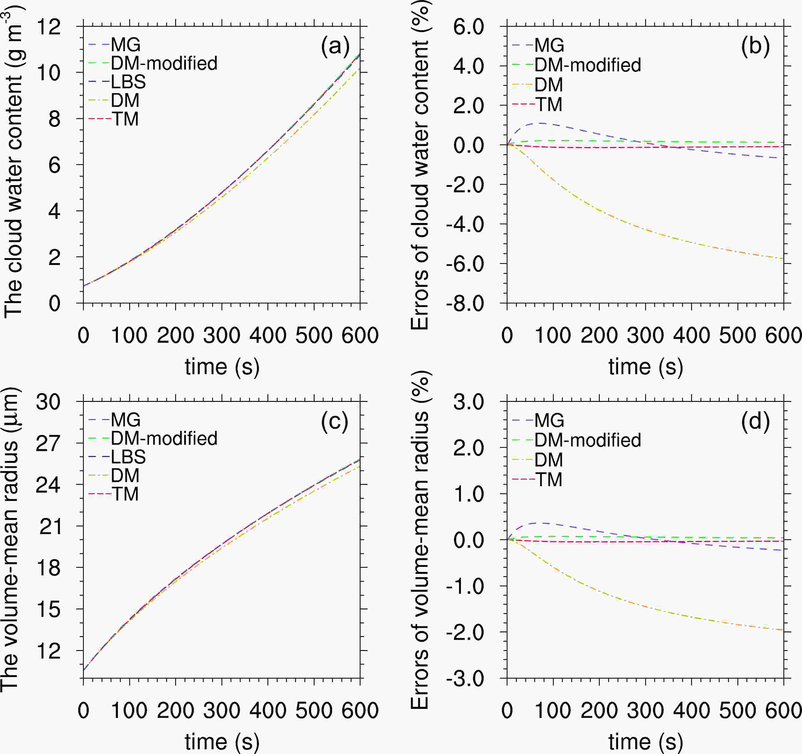
Figure 4. Same as in Fig. 3 but with the Case 2 supersaturation value of 0.3%.
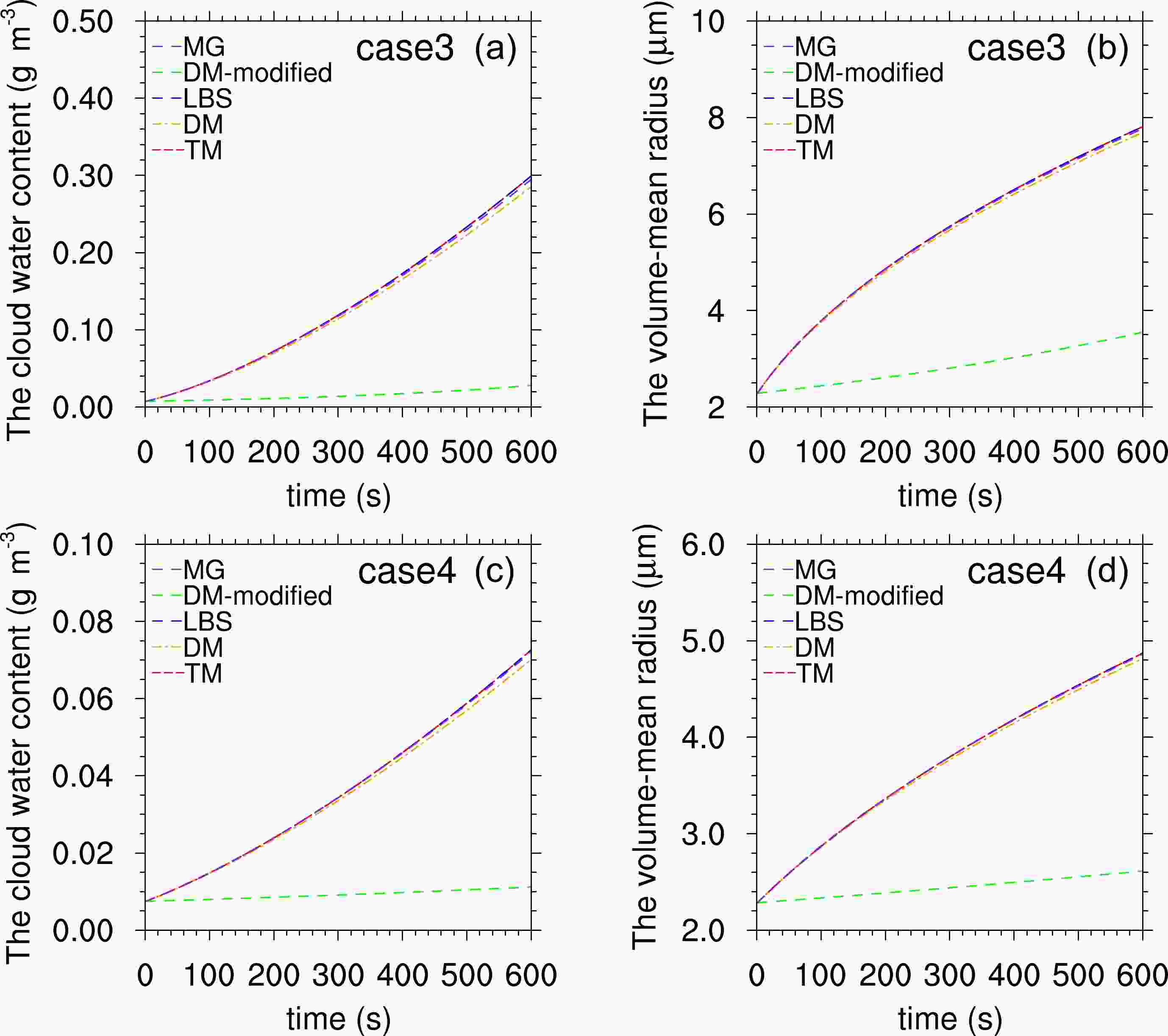
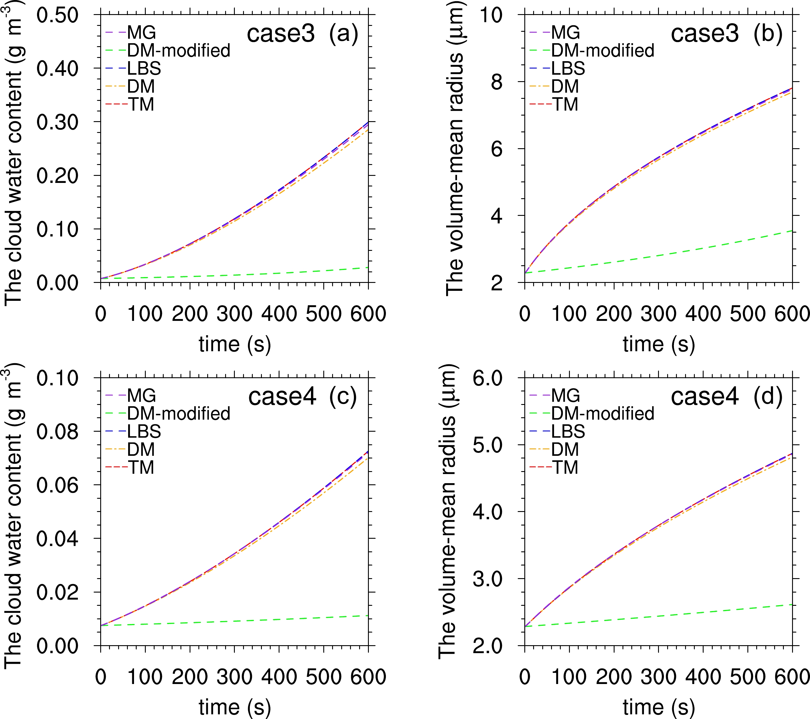
Figure 5. The evolution of the cloud water content (
$ {q}_{\mathrm{c}} $ ) and the volume-mean radius ($ {r}_{\mathrm{c}\_\mathrm{v}} $ ) with different schemes: the LBS and the DM, DM-modified, MG, and TM schemes in Case 3 and Case 4. (a) The evolution of the cloud water content ($ {q}_{\mathrm{c}} $ ) in Case 3; (b) the evolution of the volume-mean radius ($ {r}_{\mathrm{c}\_\mathrm{v}} $ ) in Case 3; (c) the evolution of the cloud water content ($ {q}_{\mathrm{c}} $ ) in Case 4; (d) the evolution of the volume-mean radius ($ {r}_{\mathrm{c}\_\mathrm{v}} $ ) in Case 4. -
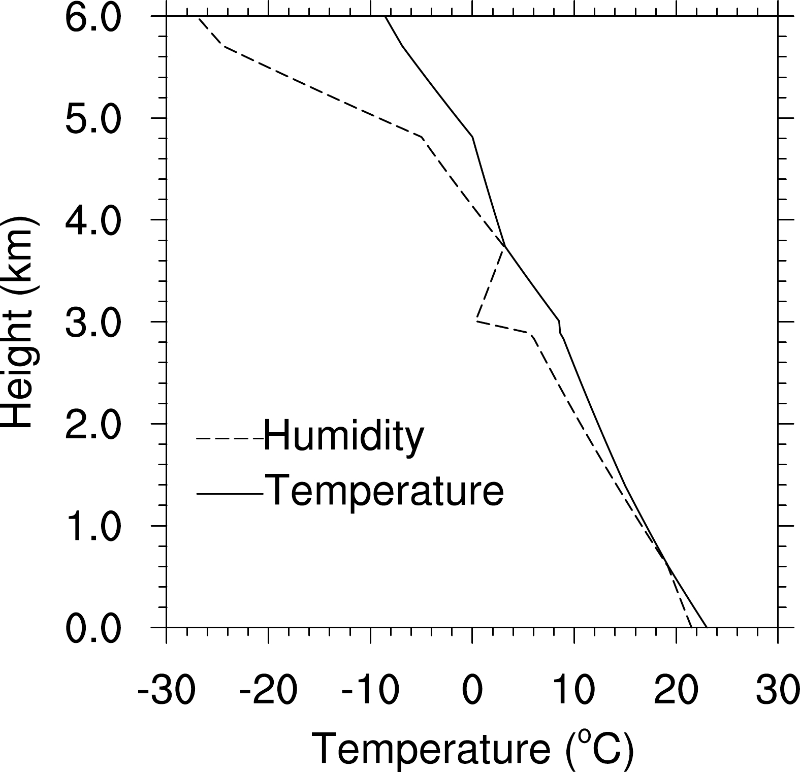
To verify the characteristics of the CDS simulated with the TM scheme in cumulus clouds, we coupled it into the 1.5D Eulerian model mentioned above. The profiles of the initial temperature and humidity fields were obtained by the observations of RICO on 16 December 2004 (Rauber et al., 2007), as shown in Fig. 6. The initial trimodal dry aerosol distribution was adopted in the model following Sun et al. (2012a). The aerosol component was assumed to be sodium chloride. Because the nucleation process needs to be taken into account in the model, a new nucleation parameterization scheme was also coupled into the 1.5D Eulerian model. The nucleation parameterization scheme can reasonably describe the activation sizes of aerosols based on a regression formula between their dry and wet radii. The following simulation only includes nucleation and condensation processes, and the vertical resolution was set to 50 m. The time steps for the dynamical and microphysical processes are 2 and 0.1 seconds, respectively.

Figure 6. The initial temperature and humidity fields. The data is obtained from the observations of RICO on 16 December 2004 (Rauber et al., 2007).
Figure 7 shows the evolution of the supersaturation, vertical velocity, and cloud water content with time and height. The simulated maximum cloud water content and vertical velocity are 1.5 g m–3 and 1.5 m s–1, respectively. The evolution of supersaturation shows that nucleation occurs at the two boundaries of cloud base and cloud top (Fig. 7a). The gradient force owing to the dynamic perturbation pressure results in the cloud-free air above the cloud top moving upwards and then becoming supersaturated (Sun et al., 2012b).
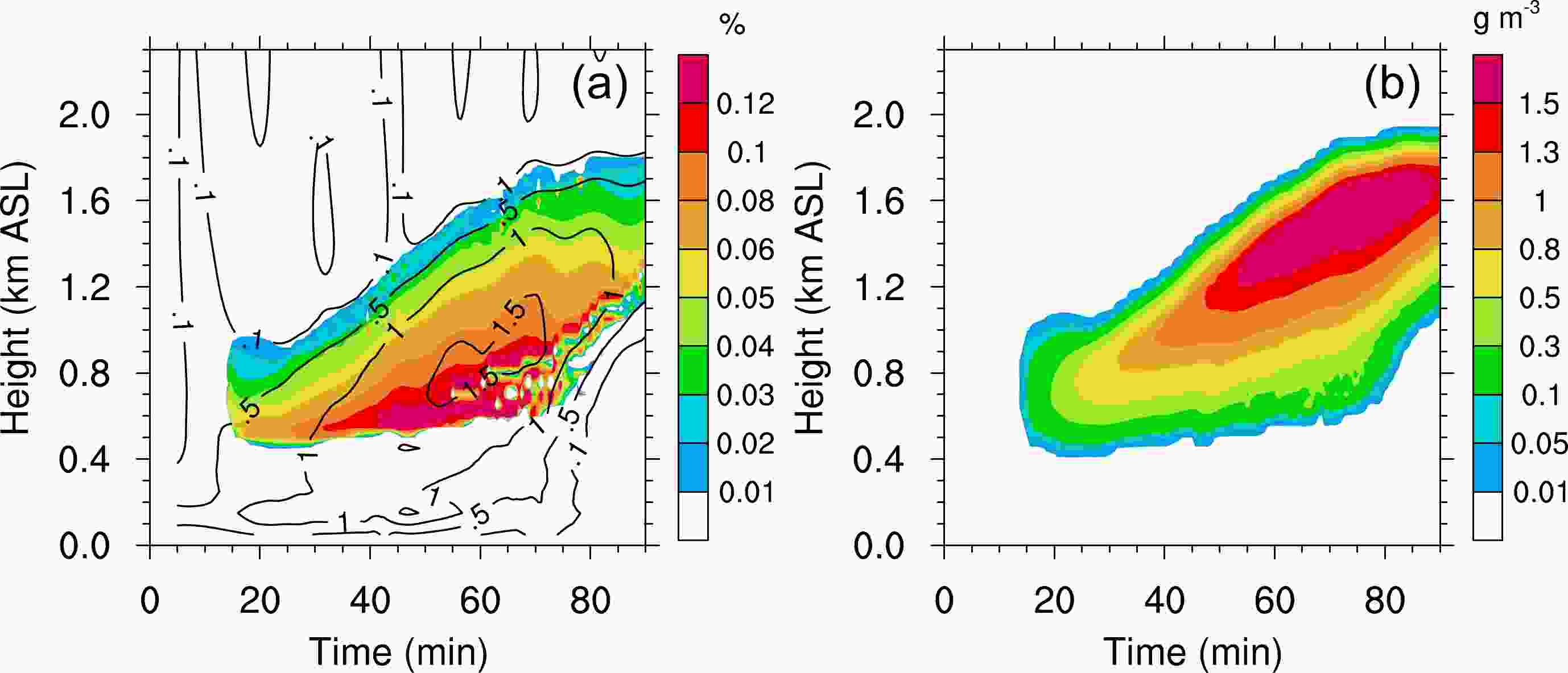
Figure 7. Temporal evolutions of the supersaturation, vertical velocity (m s–1), and cloud water content (g m–3). (a) The vertical velocity and supersaturation, where the solid lines denote the vertical velocity and the shaded area represents the supersaturation values; (b) the cloud water content.
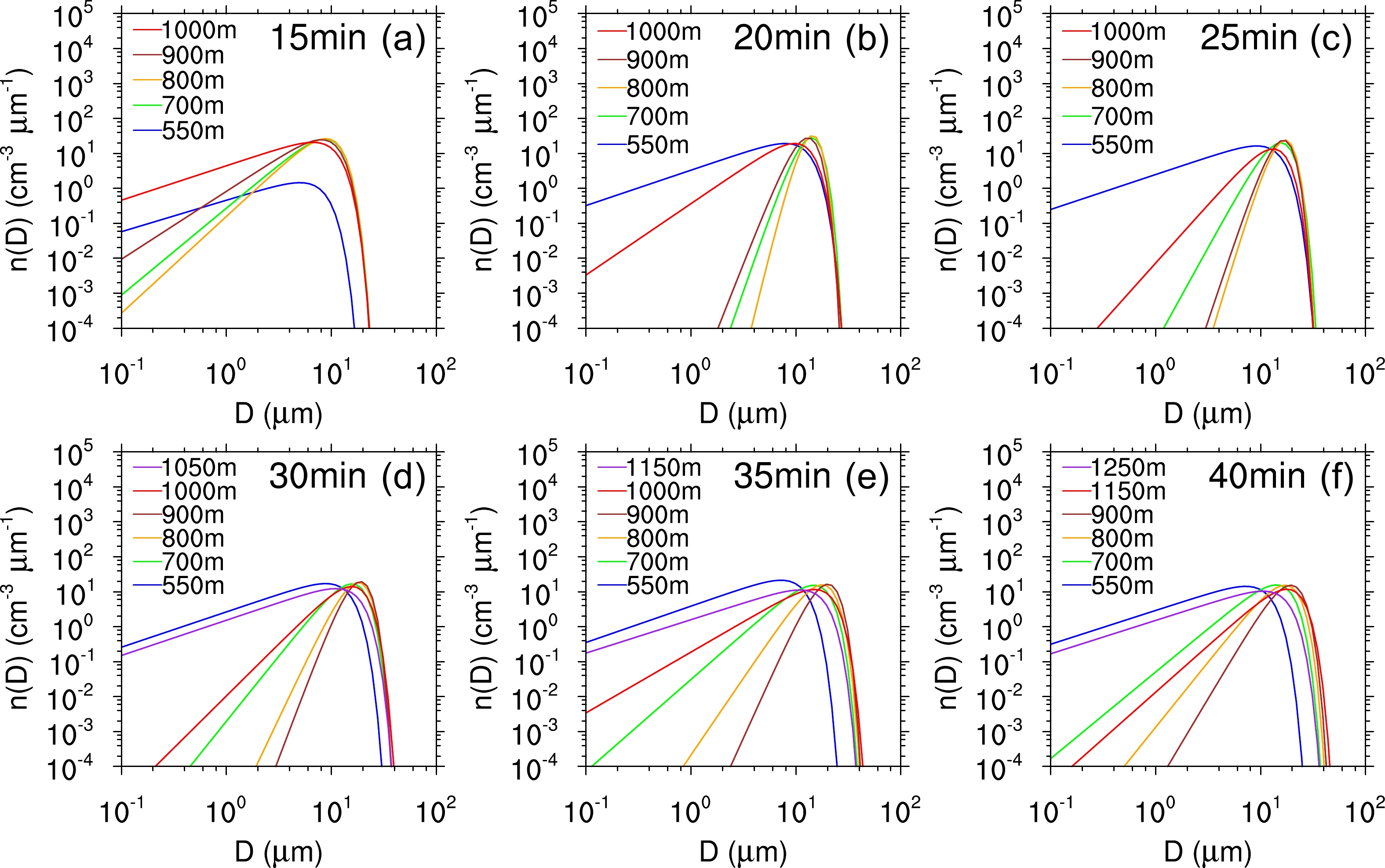
To show the characteristics of the CDS in the simulated cumulus cloud, we analyzed the cloud droplet spectra at multiple heights for the following times: 15 min, 20 min, 25 min, 30 min, 35 min, and 40 min. Figure 8 shows that the cloud droplet spectra from the newly nucleated droplets at the boundaries of the cloud base and the cloud top have wide widths. Since the supersaturation values at the cloud top are small, the nucleated cloud droplets have low concentrations, which further leads to the droplets containing giant sodium chloride particles growing fast and attaining a 40 μm size during a very short time period. Note that the cloud droplet spectra from the cloud base to the cloud top first becomes narrow and then tends to widen with height due to the condensation growth for both freshly nucleated droplets at the two boundaries.

Figure 8. Cloud droplet spectra simulated with the new scheme at the different heights for different times: (a) 15 min; (b) 20 min; (c) 25 min; (d) 30 min; (e) 35 min; (f) 40 min.
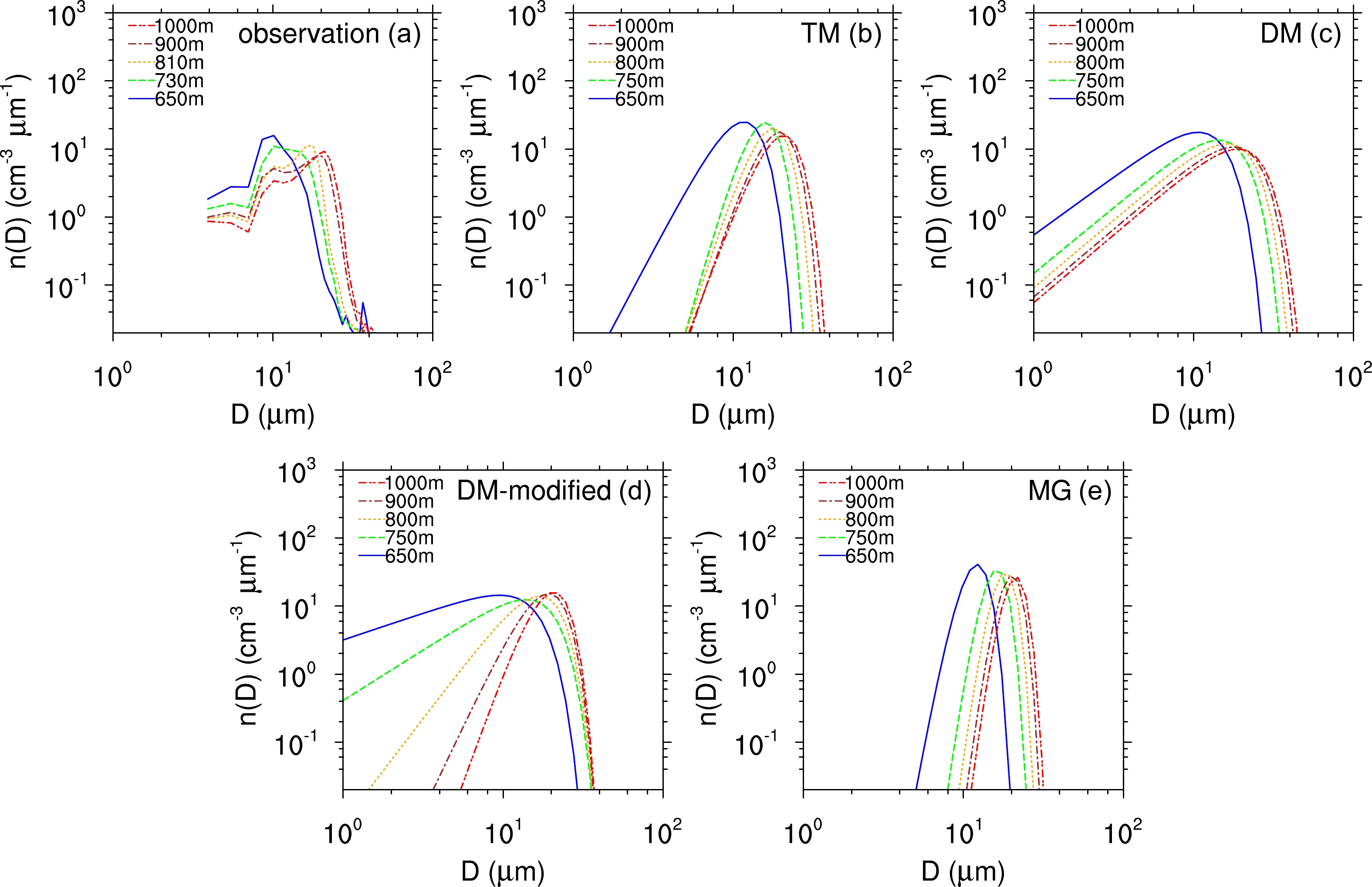
For the observation case on 16 December 2004, the C-130 airplane crossed several shallow cumulus clouds from 100 m to 500 m above the cloud base. The averaged cloud droplet spectra measured by FSSP-100 widened with increasing height (Fig. 9a). At those heights, the growth of the cloud droplets measured by FSSP-100 can be considered to have occurred mainly by condensation (Wang et al., 2016). To compare those cloud spectra with the simulation, the simulated averaged spectra by the TM, DM, DM-modified, and MG schemes at 16–20 min, 21–25 min, 26–30 min, 31–35 min, and 36–40 min, at heights of 650 m, 750 m, 800 m, 900 m, and 1000 m, respectively, were selected for comparison. Since the vertical resolution was set to 50 m in the 1.5D model, the heights of the simulated spectra are slightly different from the observations. But, in general, the simulated spectra of the new scheme are close to those in the observation. The widths of the cloud droplet spectra for both the observation and the simulation become larger with the height. However, the spectra simulated with the DM scheme are wider than those in the observation. The simulated spectra in the DM-modified scheme narrow with time, but the spectra are much wider than those in the observation at 650 m and 750 m. The simulations in the spectra with the MG scheme are narrower than the observations.

Figure 9. Evolution of the simulated and measured cloud droplet spectra. (a) The observed cloud droplet spectra from RICO; (b) the simulations of TM; (c) the simulations of the DM scheme; (d) the simulations of the DM-modified scheme; (e) the simulations of the MG scheme.
-
This study elucidated the importance of the shape parameter for the spectrum evolution of cloud droplets growing by condensation. With a fixed shape parameter, the CDS is spuriously broadened, and the number concentration of the large cloud droplets is also overestimated for the DM scheme in the idealized simulations. The overestimation may accelerate the warm rain formation. The spectra simulated with the DM-modified scheme are close to those of the LBS in Case 1 and Case 2, but they are spuriously broadened in Case 3 and Case 4. The MG scheme can improve upon the evolution of the CDS, but the CDS in the MG scheme is still wider than that in the LBS in the idealized simulations of condensation. The shape parameter is related (inversely proportional) to the relative dispersion that can be applied to describe the width of the CDS (Liu and Daum, 2000, 2002); thus, the inaccurate specification of the shape parameter is the main reason for the simulation errors of the CDS in the double-moment schemes. The shape parameter diagnosed by the number concentration, the cloud water content, and the reflectivity factor in the new scheme can overcome the spurious CDS broadening. Moreover, the treatment for the shape parameter in the new scheme reflects its flexibility and importance to the evolution of the CDS.
The errors in the simulated cloud water content (
$ {q}_{\mathrm{c}} $ ) and the volume-mean radius ($ {r}_{\mathrm{c}\_\mathrm{v}} $ ) with the new scheme are within 0.2%. However, using the fixed shape parameter to describe the Gamma size distribution can lead to –5.8%––3.3% and –2.0%– –1.5% underestimations for cloud water content ($ {q}_{\mathrm{c}} $ ) and the volume-mean radius ($ {r}_{\mathrm{c}\_\mathrm{v}} $ ) with the supersaturation values of 0.1% and 0.3%, respectively. The DM-modified scheme leads to small and steady errors for both the evolution of$ {q}_{\mathrm{c}} $ and$ {r}_{\mathrm{c}\_\mathrm{v}} $ in Case 1 and Case 2, but the simulations of$ {q}_{\mathrm{c}} $ and$ {r}_{\mathrm{c}\_\mathrm{v}} $ in the DM-modified scheme have large errors in Case 3 and Case 4. Therefore, the shape parameters diagnosed by the empirical formulas can improve the simulation of cloud droplet condensation growth; however, these schemes still have some limitations. The MG scheme can describe the cloud water content ($ {q}_{\mathrm{c}} $ ) and the volume-mean radius ($ {r}_{\mathrm{c}\_\mathrm{v}} $ ) well, but it has a constant shape parameter and overestimates the number concentration of the large cloud droplets during the idealized simulations of the condensation process. The new triple-parameter scheme can describe the condensation process of cloud droplets accurately.Furthermore, the cloud droplet spectra simulated with the DM scheme in the 1.5D model with the real sounding profile are wider than the observations. The DM-modified scheme causes the CDS to narrow with time, but the spectra are much wider than those of observations at heights of 650 and 750 m. The simulated spectra in the MG scheme are narrower than the observations. The spectra of cloud droplets simulated by the TM scheme are close to the observations. In the developing stage of the maritime shallow cumulus clouds, the cloud droplet nucleation occurs at both boundaries of the cloud base and the cloud top. The widths of the cloud droplet spectra from the cloud base to the cloud top become narrow and then may become wide with the height due to the very low concentration of cloud droplets containing giant aerosol particles to be activated.
Based on the accurate description of the CDS during condensation, the new scheme can be applied to improve the numerical simulation of the warm rain formation. In addition, the accurate description of the stochastic collision and coalescence processes is the basis of the warm rain formation. Therefore, our future paper will introduce a new warm rain formation scheme based on analytical solutions for the accretion and autoconversion rates.
Acknowledgements. This study was supported by the National Natural Science Foundation of China (Grant Nos. 41275147 and 41875173) and the STS Program of Inner Mongolia Meteorological Service, Chongqing Institute of Green and Intelligent Technology, Chinese Academy of Sciences and Institute of Atmospheric Physics, Chinese Academy of Sciences (Grant No. 2021CG0047). The authors would like to thank the three anonymous reviewers for their helpful comments that greatly improved the clarity of this manuscript.
| Cases | $ s $ | $ {N}_{\mathrm{c}} $ (cm–3) | $ {q}_{\mathrm{c}} $ (g cm–3) | $ {Z}_{\mathrm{c}} $ (cm6 cm–3) | $ \alpha $ | $ \beta $ (g–1) |
| Case 1 | 0.1% | 150 | 7.5 × 10⁻⁷ | 2.05 × 10⁻¹⁴ | 2 | 4 × 10⁸ |
| Case 2 | 0.3% | 150 | 7.5 × 10⁻⁷ | 2.05 × 10⁻¹⁴ | 2 | 4 × 10⁸ |
| Case 3 | 0.03% | 150 | 7.5 × 10⁻⁹ | 1.82 × 10⁻¹⁸ | 3 | 6 × 10¹⁰ |
| Case 4 | 0.01% | 150 | 7.5 × 10⁻⁹ | 1.82 × 10⁻¹⁸ | 3 | 6 × 10¹⁰ |


 AAS Website
 AAS WeChat