


 DownLoad:


-
The atmospheric boundary layer is defined as the lowest layer of the troposphere that is directly influenced by the forcing of the surface (Stull, 1988; Cuxart et al., 2006). Although much is known about the physical processes of the convective boundary layer (CBL) and the turbulence characteristics within it, less is known about the nocturnal boundary layer (NBL), especially regarding what happens under the presence of an urban underlying surface (UUS), when the thermal-dynamic properties are greatly changed by the urban canopy layer (UCL). Generally speaking, the radiative cooling effect from the ground leads to the gradual development of the NBL, but the development rate of this surface inversion layer could be influenced by the weather conditions such as clear skies, days with weaker winds, or days with with different cloud covers, except for the polar regions that always maintain a stable boundary layer (SBL) due to the special underlying icy surface. The NBL consists of the SBL (namely, the surface inversion layer), residual layer (RL) and capping inversion layer (Sorbjan, 1989; Glickman, 2000).
Due to the combination of weakness of much turbulence, the background noise of observation instruments and the intermittent turbulence of the SBL, the study of the SBL has developed relatively slowly from observations, numerical simulations and theoretical research (Nieuwstadt, 1984; Nappo and Johansson, 1999; Lemone et al., 2019; Liu and Hu, 2020). Current weather prediction models or climate models often overestimate the turbulence fluctuations in the SBL (Cuxart et al., 2006). The NBL simulated by models is often quite different from the observed NBL. The thermal-dynamic characteristics of the UUS would undoubtedly increase the uncertainty of the turbulence regimes of the SBL. The study of a stably stratified boundary layer over the UUS is of great significance to the local weather, climate, and especially the air quality. The poor representations of the SBL in dispersion models often produce failures in estimating pollutant concentrations in low-wind-speed conditions (Mahrt and Mills, 2009).
Because the continuous progress of atmospheric measurement technology in recent decades has promoted the widespread utilization of meteorological tower, radiosonde, tethered balloon, aircraft and remote sensing observation technologies, the understanding of turbulence regimes of the SBL over different underlying surfaces has improved (Sun, 2011; Liang et al., 2014; Bosveld et al., 2020; Mamtimin et al., 2021). Based on the experimental observation data from the Cooperative Atmospheric-Surface Exchange Study-1999 (CASE99), Sun et al. (2012) proposed the famous “HOckey stick transition” (HOST) theory available for flat areas according to the relationship between turbulent velocity scale
$ ({V_{{\rm{TKE}}}} = {[(1/2)(\sigma _u^{\text{2}}{\text{ + }}\sigma _v^{\text{2}}{\text{ + }}\sigma _w^2)]^{1/2}}) $ and mean horizontal wind speed (V). Turbulence generated by the local shear, the bulk shear and sporadic top-down bursts were defined as regime 1, regime 2, and regime 3, respectively. HOST theory reveals the transition between the SBL turbulence regime at a VT and provides a new basis for turbulence parameterization in the surface layer. In the study by Mahrt et al. (2013) of the turbulence behavior at multiple sites with different surface roughness lengths, it was shown that the wind speed threshold decreases with increasing roughness length. Russell et al. (2016) explored the relationship between turbulence and V dependence on the wind direction and canopy depth over a forest canopy. Yus-Díez et al. (2019) showed that the HOST turbulence relationships for the Boundary-Layer Late Afternoon and Sunset Turbulence (BLLAST) field campaign data were strongly dependent on both the meteorological and orographic features. Kaiser et al. (2020) reported such rapid transitions are observed in polar regions or at night and they have important consequences for the strength of mixing processes. The theory has also been investigated using large-eddy simulation (LES) models (Udina et al., 2013). The LES models have difficulties with respect to reproducing regime 1.However, most previous studies have focused on flat terrain. Whether the relationship between VTKE and V in the urban boundary layer (UBL) conforms to the HOST theory has still not been verified. With rapid urbanization, many typical megacities with dense populations, dense road networks, and developed industry and commerce have formed in recent decades. The urban surface is composed of buildings, roads, vegetation and many other different coverings. This unique complex underlying surface of the city could exert great influences on radiation processes, thermal structures, humidity characteristics, wind flows and so on in the UBL. Many kinds of urban construction consume immense amounts of energy, and consumed energy is finally converted to anthropogenic heat, continuously affecting the regional atmosphere (Li et al., 2021). The observational results have portrayed the positive nighttime sensible heat flux in the lower layer (Shi et al., 2019), indicating the great influences caused by anthropogenic heat in the UCL in winter. The UCL refers to the atmosphere near the ground layer below the top of urban buildings (Oke et al., 2017), and UCL height is defined as the average height of these buildings. From the perspective of urban climate, the UCL modulates the regional climate, including significant increases in temperature, decreases in humidity and V, and more frequent extreme meteorological disasters (Grimmond, 2007; Kaufmann et al., 2007; Li et al., 2015). Significant roughness caused by the canopy and its geometry directly influences the flow fields (Russell et al., 2016). Because the anthropogenic heat, air pollutants, and greenhouse gases emitted during human production and life activities are basically maintained near the ground, the atmospheric environment of the UCL and its corresponding urban climatology have gradually become hot topics.
In the current study, we attempt to better understand the turbulence regimes and vertical structures of the nocturnal stable boundary layer (NSBL) over the UUS. The observation data utilized in this paper are from the Beijing 325-m meteorological tower. Various tall buildings, roads and vegetation covers are distributed around the tower, thus exerting strong disturbances on the surrounding air flows. The drag shear of the buildings on the air flow in the UCL is an important source of mechanical turbulence in the NSBL. Beijing, the capital of China, is a world-famous megacity with a population of more than 21 million people. A deeper analysis of the tower data of this typical city would contribute to the improvement of the scientific theory and simulation results of the parameterization scheme of the UBL.
-
The Beijing 325-m meteorological tower (39.96°N, 116.36°E, 49 m above sea level) is located at the Institute of Atmospheric Physics (IAP, Fig. 1b) of the Chinese Academy of Sciences. This tower was built in August 1979, approximately 1 km distant from the North Third Ring Road in Beijing. The tower is still an important platform for revealing the physical and chemical properties of the atmospheric boundary layer (ABL). Since the 1990s, Beijing's urban construction has accelerated; the building area has increased exponentially, and the scale of the city has also expanded rapidly. Now, its underlying surface is a fully developed city surface (Al-Jiboori and Hu Fei, 2005; Lyu et al., 2018). Around the meteorological tower, Zhong Xin Jia Yuan and Ma Dian Jin Dian are to the north, and tall buildings such as Guan Cheng Garden and the China Science and Technology Exhibition Center have subsequently emerged to the south, changing the underlying surface around the meteorological tower from a flat area into a complex typical urban rough layer.
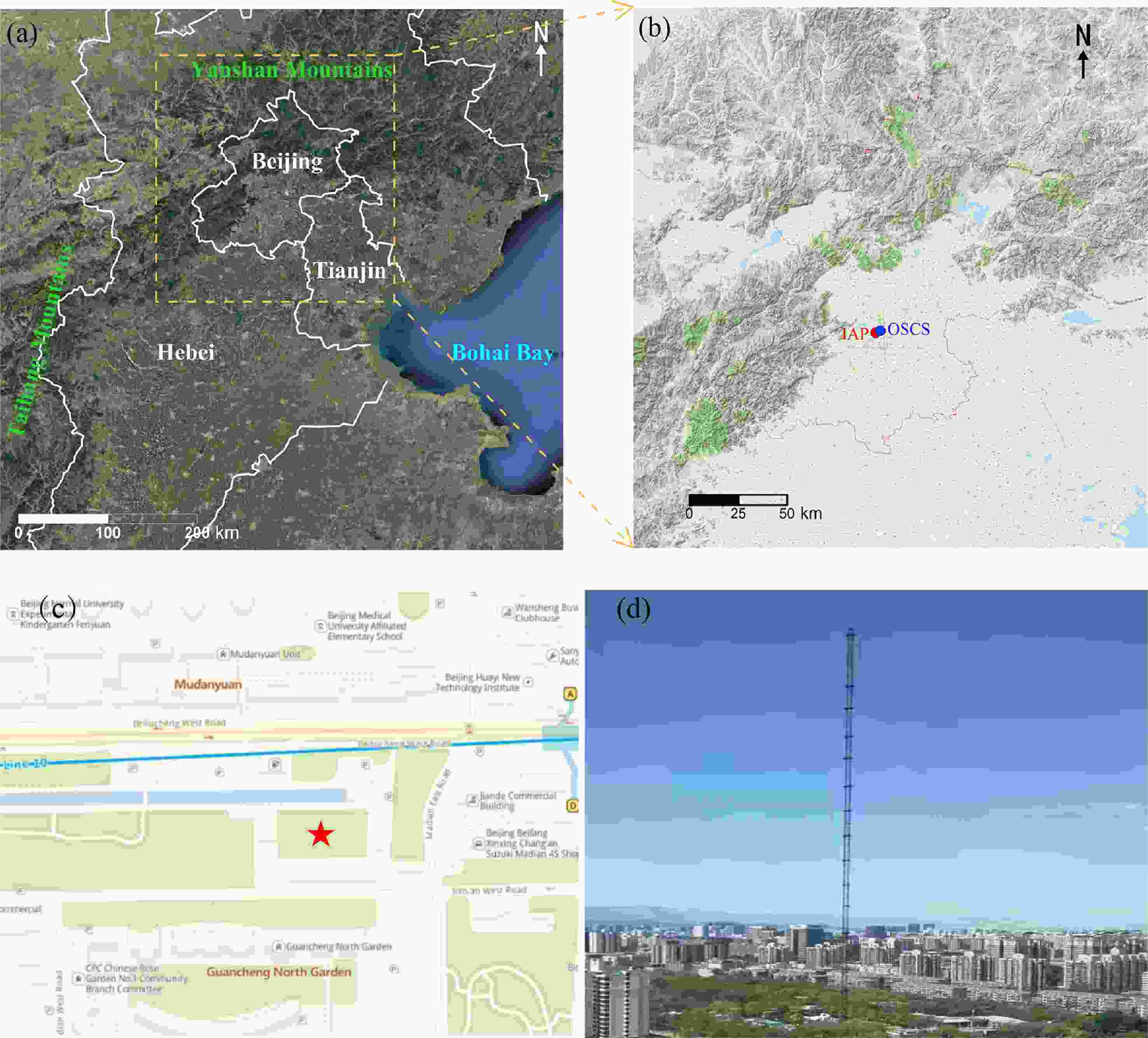
Figure 1. (a) Topography of Beijing and its surrounding area, (b) red circle represents the Institute of Atmospheric Physics (IAP) while the blue circle represents the environmental monitoring station at the Olympic Sports Center Station (OSCS), (c) distribution of the buildings around the tower; and (d) photograph of the Beijing 325-m tower.
The height of urban canopy is generally recognized as the distance from the ground to the building roof (Oke et al., 2017). Theoretically, surrounding flows could reflect the impacts of such buildings, and then the canopy height can be estimated. The UCL height around the observation tower is approximately 80 m according to the average height of the surrounding buildings (He et al., 2019). The most important building near the tower is Guan Cheng Garden, approximately 100 m away from the meteorological tower to the south (shown in Fig. 1c). This garden is divided into two parts, and the height of the buildings is estimated to be approximately 80 m. There are 15 observation platforms (at 8, 15, 32, 47, 65, 80, 103, 120, 140, 160, 180, 200, 240, 280, and 320 m) equipped on the tower (shown in Fig. 1d seen in Table 1), and each platform is mounted with instruments to measure wind speed (MetOne, USA), wind direction (MetOne, USA), temperature (HC2-S3, Switzerland), and humidity (HC2-S3, Switzerland). Seven levels (8, 15, 47, 80, 140, 200, and 280 m) containing three-dimensional ultrasonic anemometers (Wind Master, Gill, UK) and open path gas analyzers (LI-7500A, LI-COR) for measuring water vapor and CO2 concentrations are located on the tower, with a sampling frequency of 10 Hz.
Surface measurements of PM2.5 (particulates with aerodynamic diameters less than 2.5 µm) concentrations at the Olympic Sport Center Station (OSCS, shown in Fig. 1b), approximately 2 km from the IAP, were downloaded from the official website of the Beijing Environmental Protection Agency (
http://beijingair.sinaapp.com/ ). -
The observation data from 1 November (Nov) 2017 to 31 January (Jan) 2018 were utilized this paper. All data and results in this study are presented at Beijing Standard Time (LST= UTC + 8 h). To conveniently express and analyze the data, some parameters and symbols used in this paper are explained here, and the corresponding calculation formulas are also given. The longitudinal, lateral, and vertical velocity standard deviation
$ {\sigma }_{u},{\sigma }_{v},{\sigma }_{w} $ and turbulence kinetic energy (TKE) are calculated as follows:where u, v, and w are the longitudinal, lateral and vertical components of wind, respectively, and turbulence fluctuations are computed by
${x}'=x-\overline{x}$ ,$\overline{x}$ representing Reynold’s averaging over a 30 min period in this paper. Generally, the averaging time of SBL turbulence at night is between 5 and 20−30 min. However, the period studied in this paper included several heavy pollution events, which occurred under stagnant synoptic weather systems, and the evolution of SBL structure was noticeably slower. In addition, the sampling frequency of PM2.5 concentration used in this paper was 30 min. Therefore, we used 30 min as the averaging time.The skewness of the vertical wind component is calculated as follows:
The probability distribution of truly random homogeneous isotropic turbulence should be Gaussian or quasi-Gaussian, and its skewness value should be zero (Jacobs et al., 2001). However, in the actual atmosphere, due to the influence of various factors, such as large-scale synoptic systems, nonstationary flow or the influence of heterogeneous underlying surfaces, the statistical values of atmospheric turbulence deviate from a Gaussian distribution. For the purposes of this study, skewness can quantitatively describe the deviation degree between this random process and the Gaussian distribution. Determining the distribution of the turbulence flows inside and outside the urban canopy could deepen the understanding of the exchange process mechanism between land–air and the UUS and improve the simulation performance of the boundary layer parameterization scheme.
If positive extremes dominate, the skewness is positive, and if negative extremes dominate, the skewness is negative. Positive skewness-w indicates that the turbulence exchange process is dominated by ejection, and negative skewness-w indicates that the exchange process is affected by the sweep process.
In the following expressions,
$ {\theta }_{v} $ represents the air virtual potential temperature,$\overline{{w}^{'}{\theta }_{v}^{'}}$ is the kinematic heat flux$ ,{\theta }_{z0} $ is the potential temperature of the reference at 8 m,$ \theta \left(z\right) $ is the potential temperature at each height, and the local Monin–Obukhov scaling length Λ represents the stability condition:where subscript “l” denotes the local value,
$ {u}_{*l} $ is the local friction velocity to distinguish it from the surface friction velocity$ {u}_{*} $ , and κ is the von Kármán constant (0.35). This paper focuses on the SBL cases in the NBL, where the nighttime data are defined as being from 1800 LST to 0600 LST according to the local sunrise and sunset. The SBL is divided according to the stability parameter when$ z/\varLambda $ >0. -
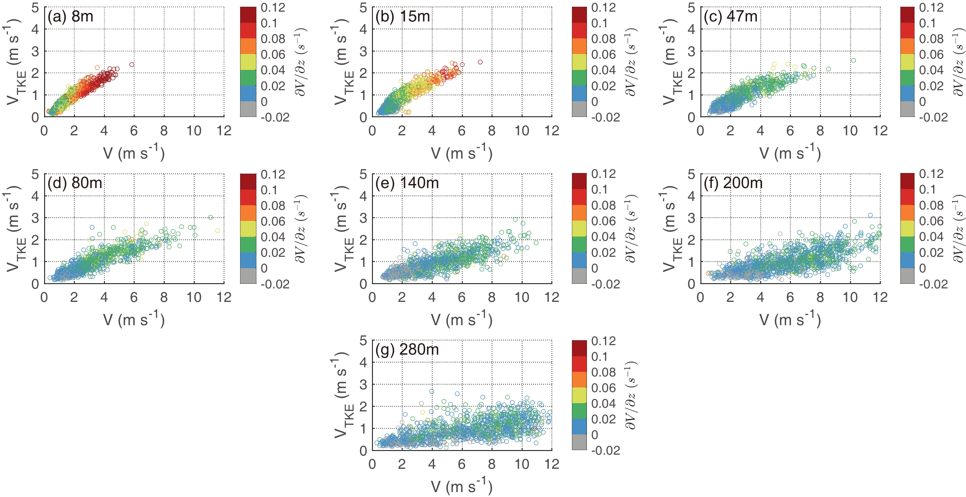
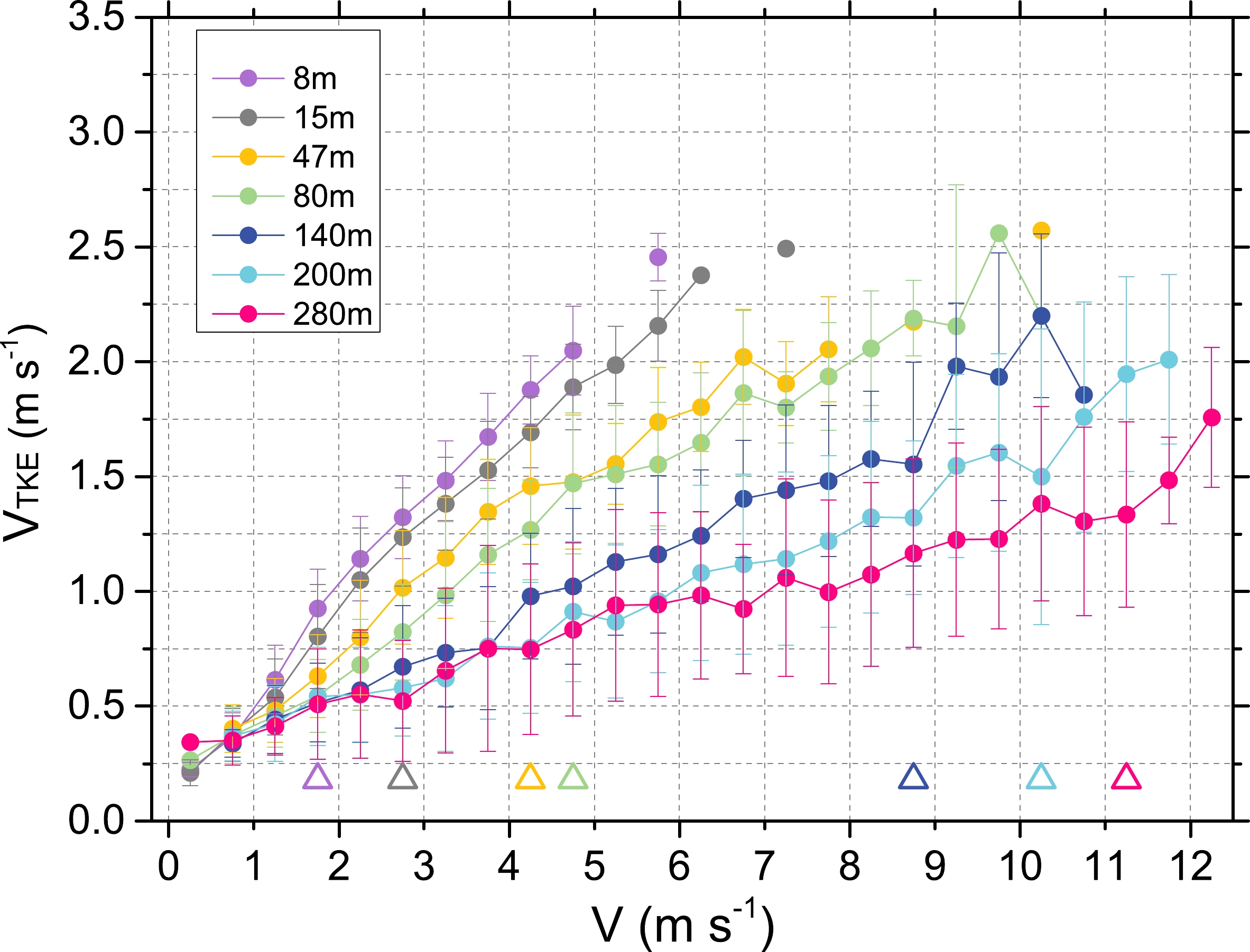
Sun et al. (2012) used 9 levels of observation data on a 60-m tower in the CASE-99 experiment over flat terrain to investigate the relationship between VTKE and V. Obviously different from the CASE-99 experiment, the observation data used in this paper were from a 325-m meteorological gradient tower in Beijing, located on the typical UUS. Figure 2 shows the relationship between VTKE and V at 7 levels on the 325-m tower, and Fig. 3 further shows the relationship between the bin-averaged turbulence strength VTKE and wind speed V. These analyses show that, in contrast with the relationship between VTKE and V from Sun et al. (2012), the relationship between VTKE and V for the 325-m tower can be divided into two types. At 8, 15, 47 and 80 m, the VTKE was very sensitive to the variation in V when V<VT, whereas VTKE increased relatively slowly with V when V>VT. The 8, 15, and 47 m measurement heights were located within the UCL, and 80 m was approximately the UCL height according to the average height of the buildings around the tower. VTKE at these four heights was greatly influenced by the drag shear of the buildings on the air flow in the UCL; thus, VTKE was partly enhanced when V was not high. The estimated wind speed threshold VT for each height (triangles shown in Fig. 3) was based on the largest change of the bin-averaged turbulence strength VTKE difference intervals
$ \Delta {V}_{{\rm{TKE}}}={V}_{{\rm{TKE}}}(V+0.5)-{V}_{{\rm{TKE}}}\left(V\right) $ .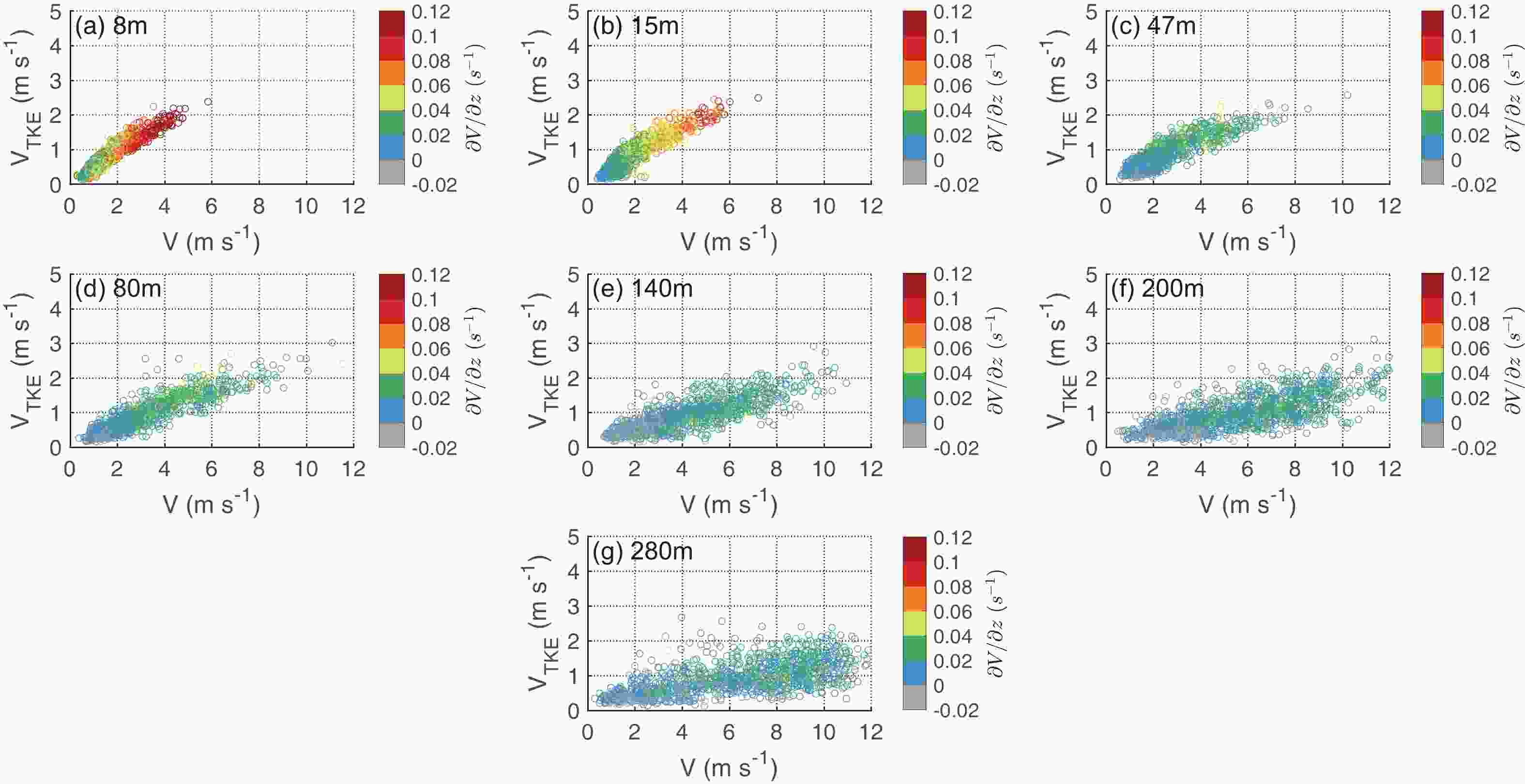
Figure 2. The relationship between the turbulence strength VTKE and wind speed V at seven observation levels the Beijing 325-m meteorological tower. The local shear value
$ \partial V/\partial z $ is used to denote the color of the scatter points.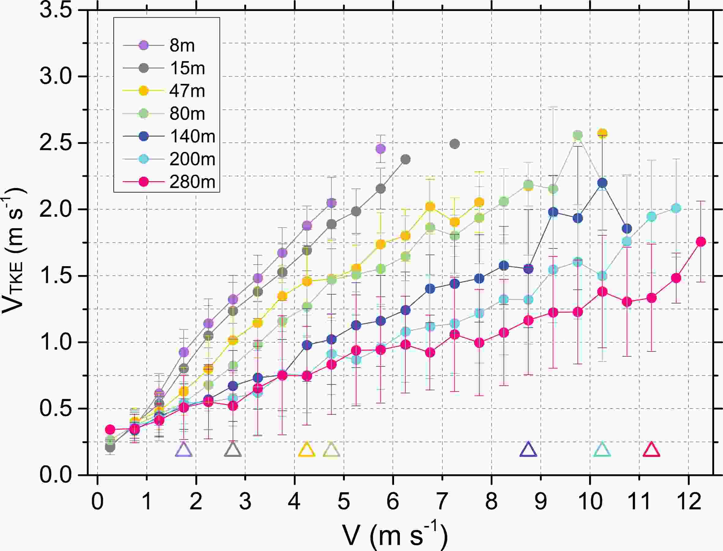
Figure 3. The relationship between the bin-averaged turbulence strength VTKE and wind speed V at seven observation levels on the Beijing 325-m meteorological tower. The threshold wind speed VT at each level is marked with a triangle in the color of the height.
A different pattern is noticeable for 140, 200 and 280 m, which is far above the UCL height. Plots of VTKE vs. V at these three heights were more consistent with those obtained by Sun et al. (2012) based on flat underlying surfaces and the results from Yus-Díez et al. (2019) based on complex terrain, in that VTKE was not very sensitive to V and increased slightly with V at 140, 200 and 280 m when V<VT. The variations of VTKE showed a close relationship with V and increased rapidly when V>VT.
Some scattered points obviously did not conform to the above pattern. Moderate turbulence could often be generated for relatively low values of V (regime 3). This otherwise weak turbulence mainly occurred at 140, 200 and 280 m above the canopy. For regime 3, turbulence may correlate with the upside-down structure in the SBL, in which the TKE at a higher altitude associated with strong wind shear is transported downward toward the surface (Mahrt and Vickers, 2002; Banta et al., 2006; Sun et al., 2012; Shi and Hu, 2020); therefore, the turbulence could be enhanced when V<VT. The top-down structure was a special kind of upside-down structure because the maximum TKE occurred at the top of the ABL. The higher TKE in the upper layer may be attributed to different causes, such as Kelvin–Helmholtz instabilities (Newsom and Banta, 2003), gravity waves (Udina et al., 2013), or low-level jets (Karipot et al., 2008), which could generate turbulence aloft.
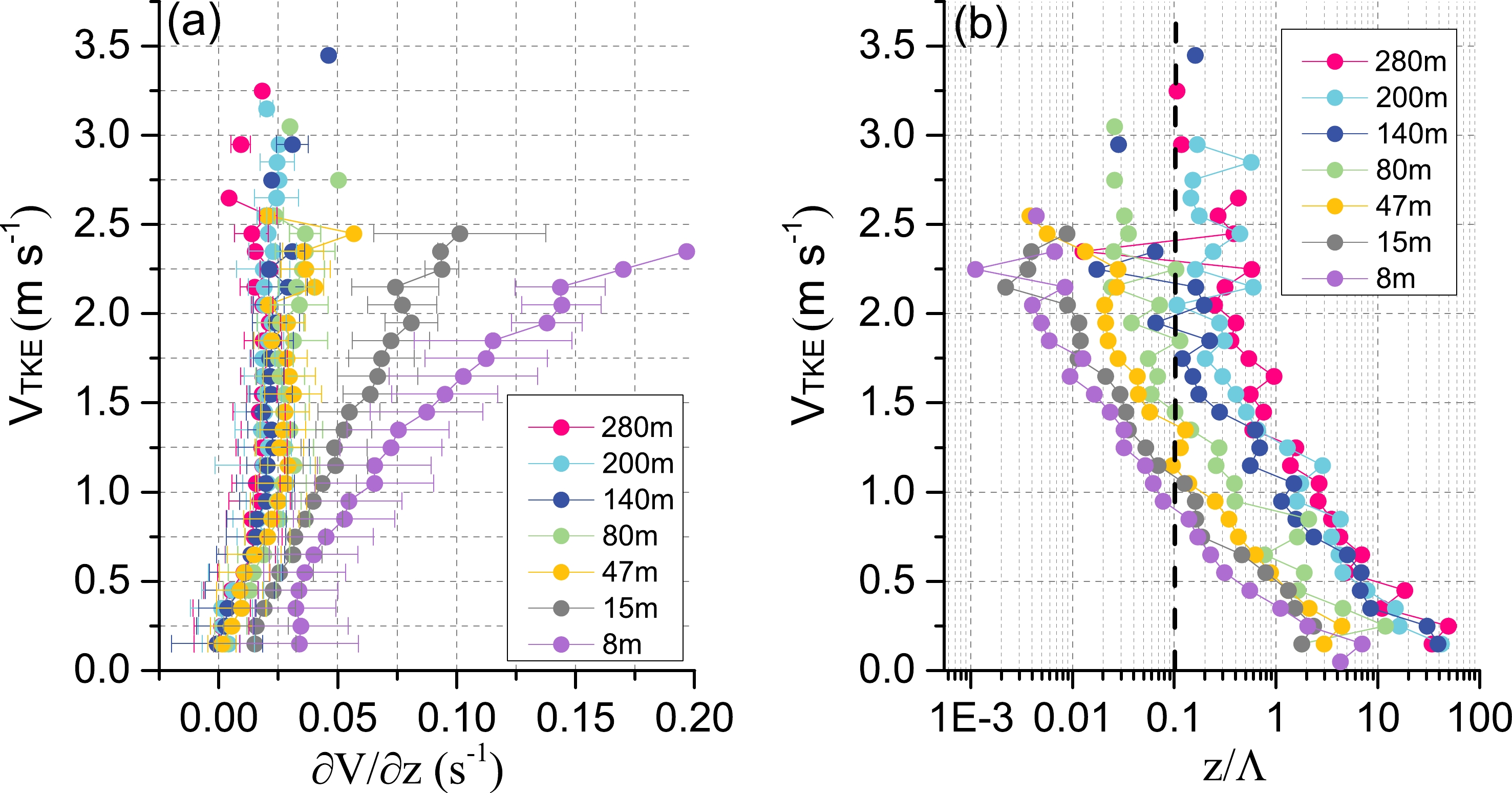
The local shear value
$ \partial V/\partial z $ is used to denote the color of the data points in Fig. 2. Due to the wind shear effect of the uneven underlying surface in the UCL on the air flows, the wind shear values at 8 and 15 m were also significantly higher and$ \partial V/\partial z $ showed a close relationship with VTKE. Weak turbulence in the lower part of the UCL was always strongly affected by local wind shear when V<VT (regime 1). Figure 4a further shows a strong relationship between$ \partial V/\partial z $ and VTKE in the lower UCL, and the influence of the local wind shear still exists when V>VT. As shown in Fig. 4b, the weak turbulence regime with small eddies mostly corresponded to stable stratification with z/Λ>0.1.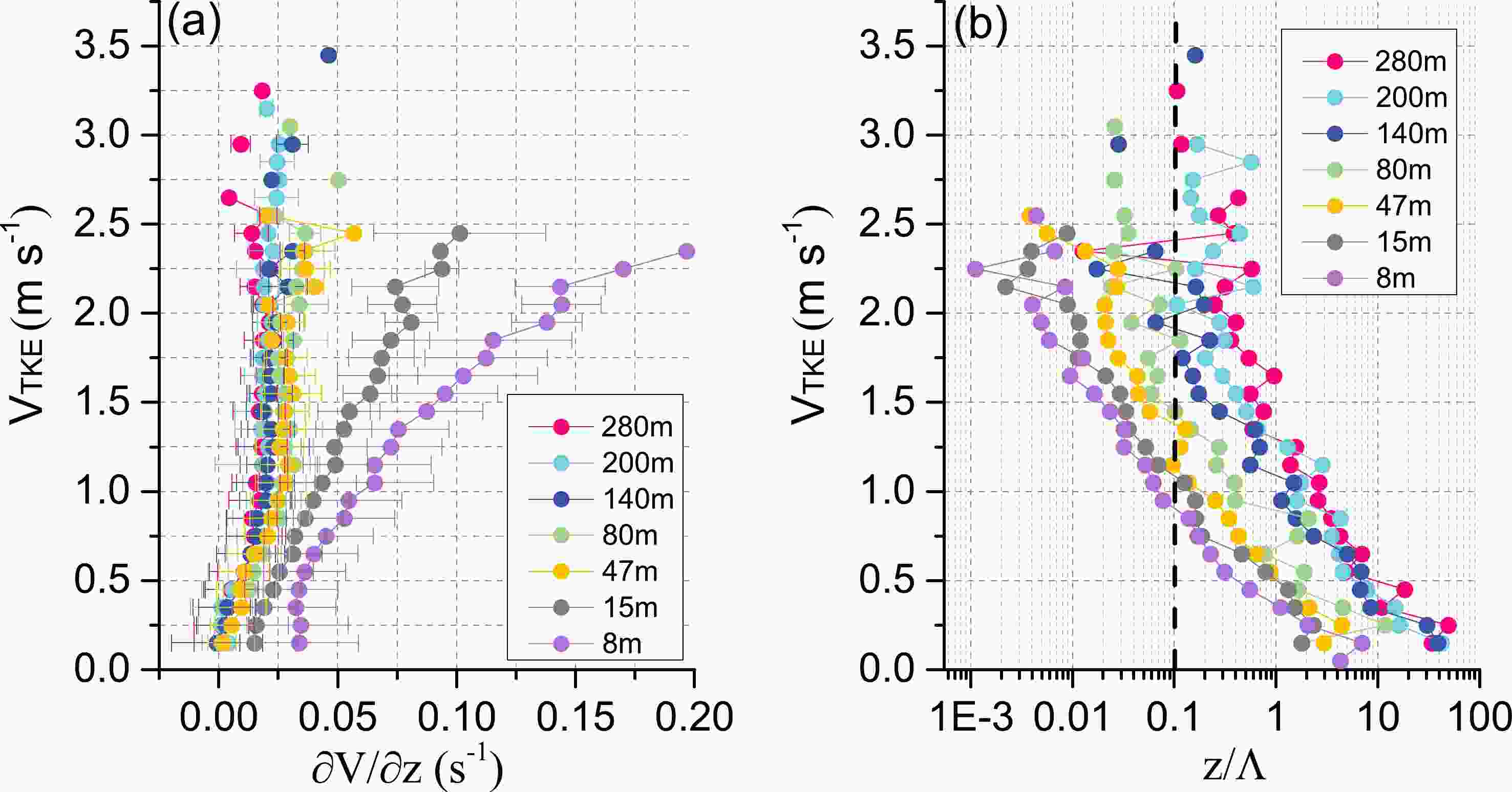
Figure 4. The relationship between VTKE and local shear
$ \partial V/\partial z $ (a) and the relationship between VTKE and stability parameter z/Λ at the seven observation levels of the 325-m meteorological tower.For heights above 47 m, when the VTKE was not very strong (VTKE < 1 m2 s−2), the VTKE increased synchronously with increasing local wind shear. However for strong turbulence, stratification approached near neutral (shown in Fig. 4b) as defined by
$ \left|z/\varLambda \right| $ <0.1, and the local wind shear had little effect on VTKE. When V>VT, as shown in Fig. 2 and Fig. 4a, although local shear still had an effect on the turbulence strength in the lower part of the UCL, the turbulence intensity in the upper layer had little relationship with local shear and the turbulence activities were mainly affected by bulk shear with strong winds (regime 2).Generally, for the flat area or where there was no obvious source of anthropogenic heat, the kinematic heat flux
$ \overline{{w}^{{'}}{\theta }_{v}^{{'}}} $ in the NSBL was negative, and the temperature gradient ($ \Delta \theta /\Delta z $ ) was positive. A higher$ \Delta \theta /\Delta z $ indicates a more stable stratification; thus, the generation of turbulence activities might be inhibited. However, as shown in Fig. 5, there were many thermally unstable stratification cases ($ \Delta \theta < 0 $ ) at night for the UBL, and this may be because of the existence of many anthropogenic heat sources in the urban canopy, such as residential heating in winter and emissions from traffic activities.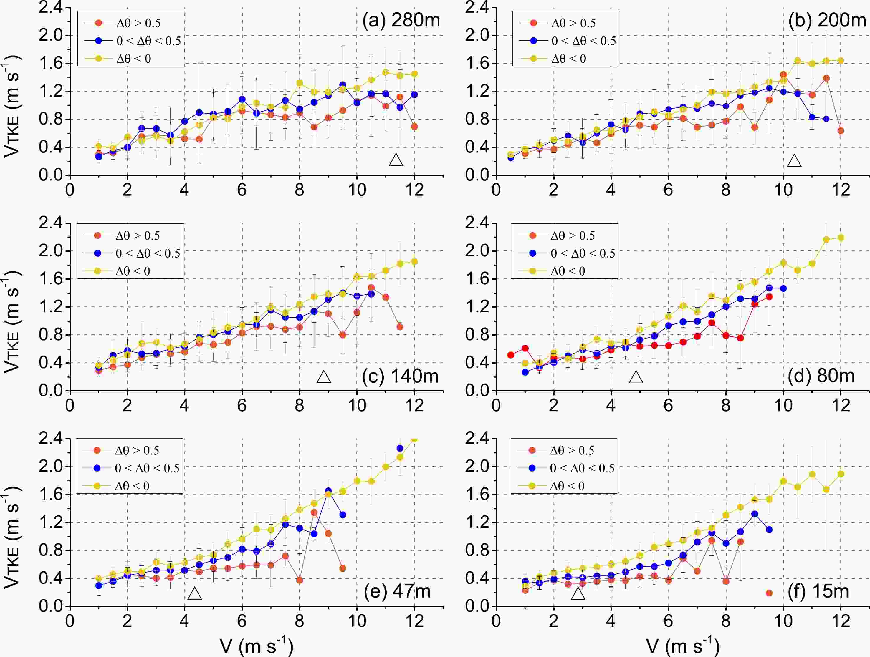
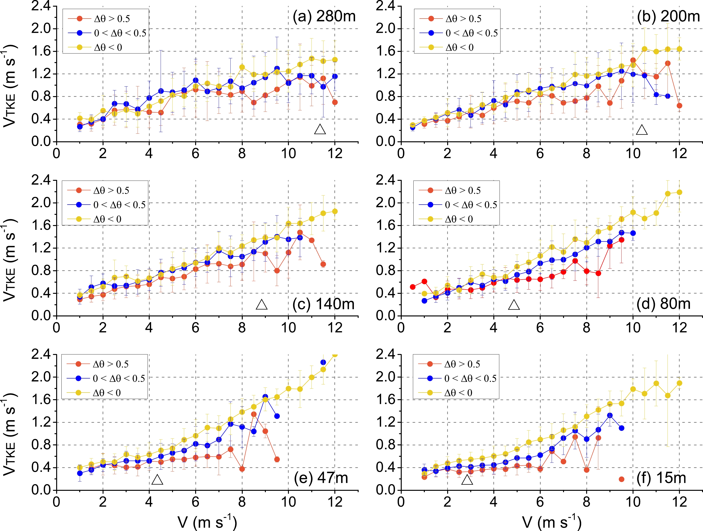
Figure 5. The relationship between the bin-averaged turbulence strength VTKE and the wind speed V at the seven observation levels as a function of potential temperature difference intervals, defined as
$ \Delta \theta =\theta \left(z\right)-{\theta }_{z0} $ , where$ {\theta }_{z0} $ is the potential temperature of reference at 8 m, and$ \theta \left(z\right) $ is the potential temperature at each height z: (a) 280 m, (b) 200 m, (c) 140 m, (d) 80 m, (e) 47 m, and (f) 15 m. The wind speed threshold VT is marked using a black triangle for each height.This paper focuses on the NSBL, and the stable cases were classified according to the local Monin–Obukhov length Λ, that is, z/Λ greater than zero. Nevertheless, as described above, when z/Λ was greater than zero at night (namely, negative sensible heat flux) and the temperature gradient
$ \Delta \theta /\Delta z $ remained negative, it indicates the emergence of counter gradient transportation of heat in the nighttime UBL (especially in UCL). The heat was transmitted from the layer with low temperature to the layer with high temperature. Counter gradient transport may be related to multi-scale vortex motions, especially turbulent coherent structures, which are not well understood (Zhou et al., 2018; Zhang et al., 2021; Shi et al., 2022).Figure 5 shows that the nighttime strong turbulence activity in winter was commonly accompanied by thermal instability (yellow line,
$ \Delta \theta /\Delta z < 0 $ ), especially for the lower layers of the UBL, such as 15, 47 and 80 m. Obviously, the lower region of the UBL was more likely to be affected by the thermal properties within the canopy. In fact, the probability of thermal instability stratification at 15–47 m exceeded 50% (54% for 15 m, 58% for 47 m). Therefore, for nighttime turbulence of the lower layer in the UBL, in addition to the contribution of local shear (regime 1) and bulk shear (regime 2), strong turbulence was also generated by buoyancy turbulence caused by anthropogenic heat, which we refer to as regime 4 in this paper.It is interesting that VTKE vs. V under three temperature stratifications (
$ \Delta \theta > 0.5;0 < \Delta \theta < 0.5;\;\mathrm{a}\mathrm{n}\mathrm{d}\;\Delta \theta < 0 $ ) were very similar when V<VT. Indeed, external effects such as temperature stratification have impacts on the turbulence regime transitions (Van de Wiel et al., 2017; Holdsworth and Monahan, 2019). The relationship between VTKE and V under the three temperature stratifications gradually separated from each other, showing great differences when V>VT. Compared with the turbulence in regime 1, the turbulence in regime 2 showed a closer relationship with thermal stratification.The red line indicates the strong stable stratification (
$ \Delta \theta > 0.5 $ ), and the turbulence intensity in this stable stratification was obviously suppressed. However, for strong stable stratification, sporadic strong turbulence could also occur. -
The TKE upside-down phenomenon often appears in the NSBL. Sun et al. (2012) attributed this moderate turbulence generated for relatively low values of V as regime 3 where turbulence may correlate with the upside-down structure in the SBL. Different from the traditional nocturnal SBL characterized by the upward transport of turbulent energy (downside-up), the most prominent feature of upside-down SBL is that the turbulence momentum flux at the higher altitude associated with strong wind shear transports downward toward the surface (Mahrt, 1999). Three typical urban SBL structures were classified according to the vertical profile of TKE (Shi and Hu, 2020).
The selection of TKE threshold is very important for the division of three types of SBL and in our study this threshold TKE was determined based on the relationship between TKE and PM2.5 concentration. The TKE values were very small during heavy haze pollution days, basically less than 1 m2 s−2 (Han et al., 2018; Shi et al., 2019; Wang et al., 2019). At this time, the atmospheric diffusion capacity was poor and the vertical exchange of turbulence momentum between different layers was very weak (weak-transport). Previous study shows that when PM2.5 exceeded 75 μg m−3, reaching national pollution standards according to the Technical Specification for Air Quality Index (HJ633-2012), the TKE at three heights (47, 140 and 280 m) of the Beijing 325-m tower was basically less than 1m2 s−2, and during heavy pollution period, TKE was basically less than 0.5 m2 s−2. According to the three-month observation period in our study, statistical results show that when PM2.5 concentration exceeded 75 μg m−3, more than 80% of the TKE at 8 m was less than 0.5 m2 s−2. If the threshold TKE was 1 m2 s−2, the probability could exceed 80%, but the high TKE value may not be able to select a typical weak-transport type. Threshold TKE value 0.1 m2 s−2 conformed to a typical weak-transport, but observation results show that when the air quality reached the polluted level, TKE was not always less than 0.1 m2 s−2. Therefore, this paper selected 0.5 m2 s−2 as a threshold value, and a TKE less than 0.5 m2 s−2 in the whole tower layer was classified as a weak-transport type. The case in which the maximum TKE in the tower layer exceeded 0.5 m2 s−2 and the maximum value appeared at the highest layer (280 m) was divided into the upside-down type. Although this division included some non-typical cases, the occurrence of the maximum TKE at the highest layer still indicated a trend of higher TKE in the upper layer. The remaining cases were divided into the traditional urban SBL type (downside-up).
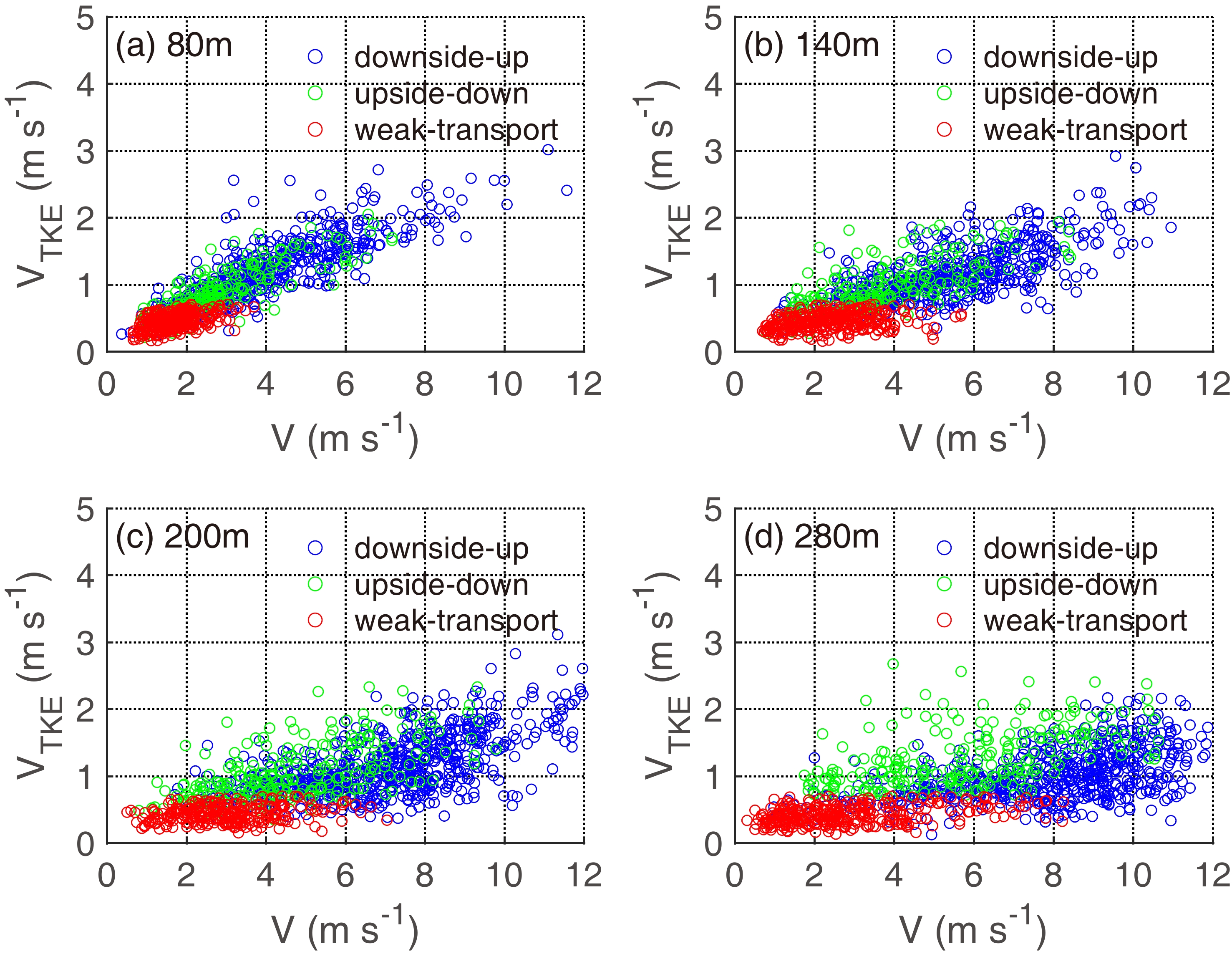
As shown in Fig. 6, in the urban SBL at night, the frequency of downside-up was highest; the probability of the weak-transport type was approximately 34%, and the upside-down type occurred the least, with a probability of approximately 16%. When an upside-down structure occurred, some moderate strength turbulence activities above 140 m (including 140 m) were observed when V<VT. This phenomenon was more obvious at higher heights, such as 200 and 280 m. Upside-down structures led to a significant enhancement of turbulence above the UCL, generating regime 3. However, the turbulence enhancement was not obvious below the UCL height.

Figure 6. The relationship between the turbulence strength VTKE and the wind speed V at (a) 80 m, (b) 140 m, (c) 200 m, and (d) 280 m. The red, green and blue circles represent three kinds of stable boundary layers according to the vertical profile of TKE: weak transport, upside-down and downside-up, respectively. The three patterns were classified according to the vertical profiles of TKE.
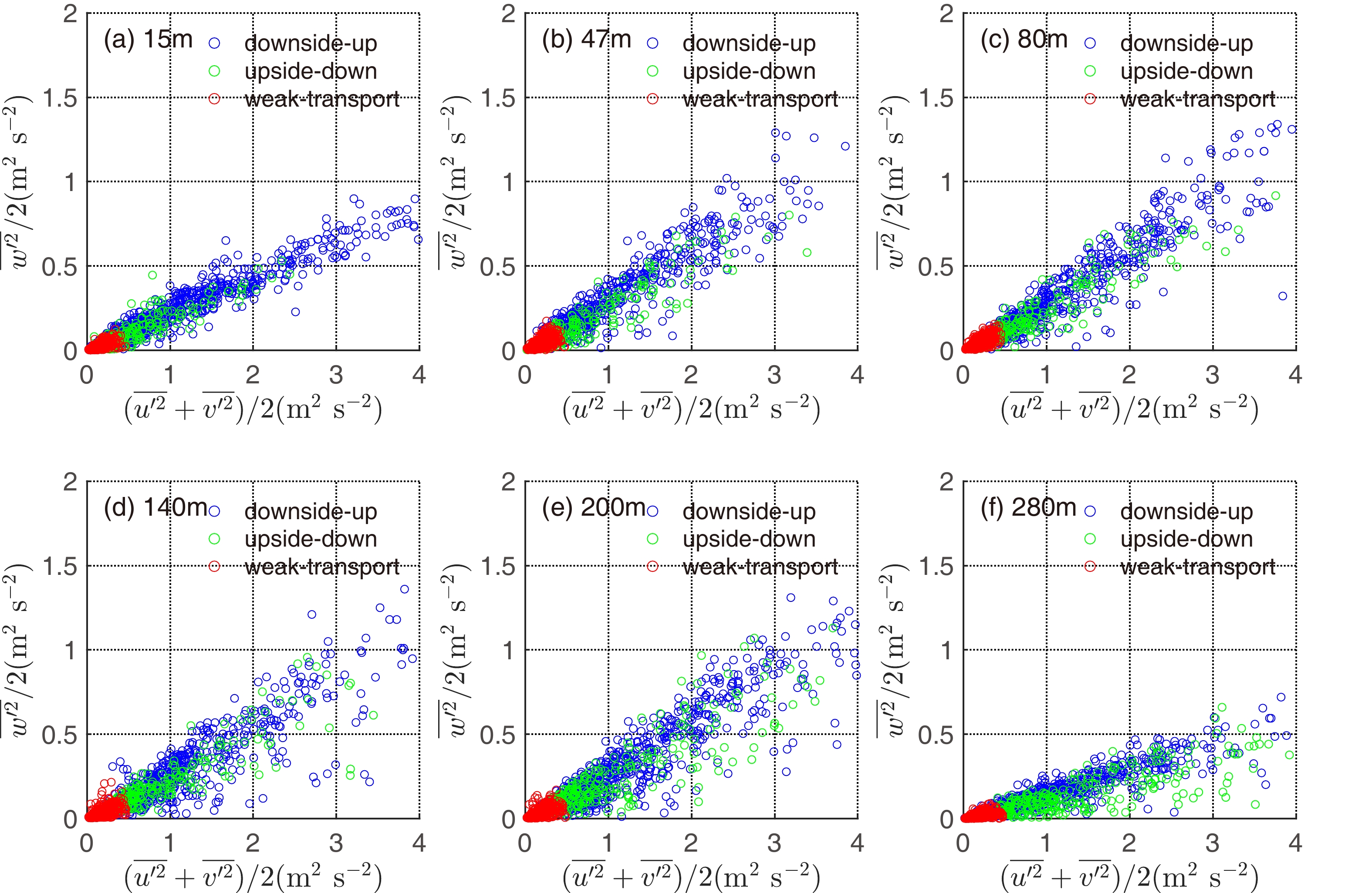
The horizontal TKE and vertical TKE were also compared. As shown in Fig. 7, the horizontal TKE was always considerably higher than the vertical TKE component, especially at 280 m, indicating that the atmospheric turbulence in the urban SBL was always anisotropic. The magnitude of the horizontal TKE increased significantly above 80 m for the upside-down structures; therefore, the upside-down structures had a higher downward transmission efficiency of the horizontal TKE than the vertical TKE.
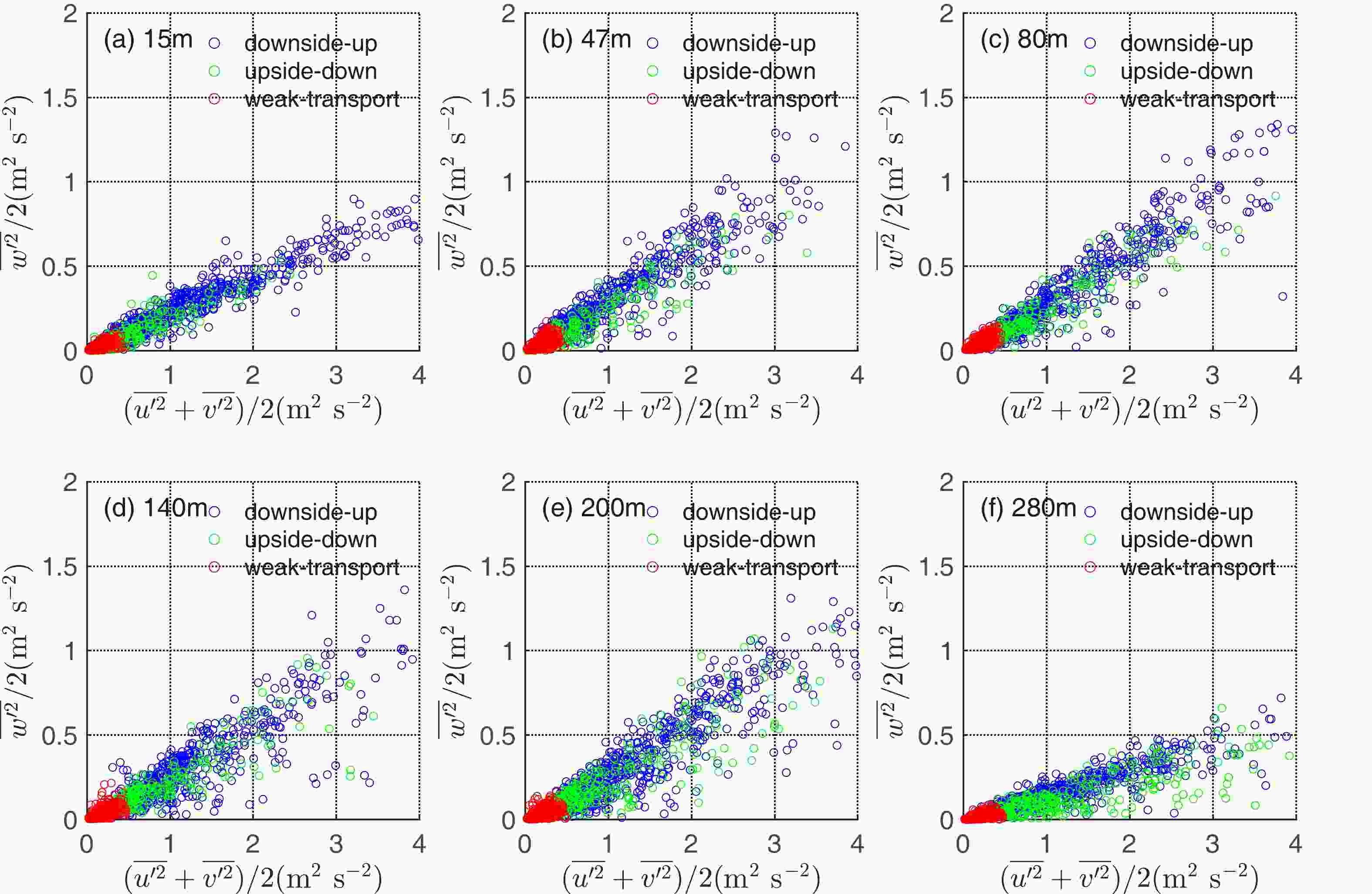
Figure 7. The relationship between the horizontal TKE
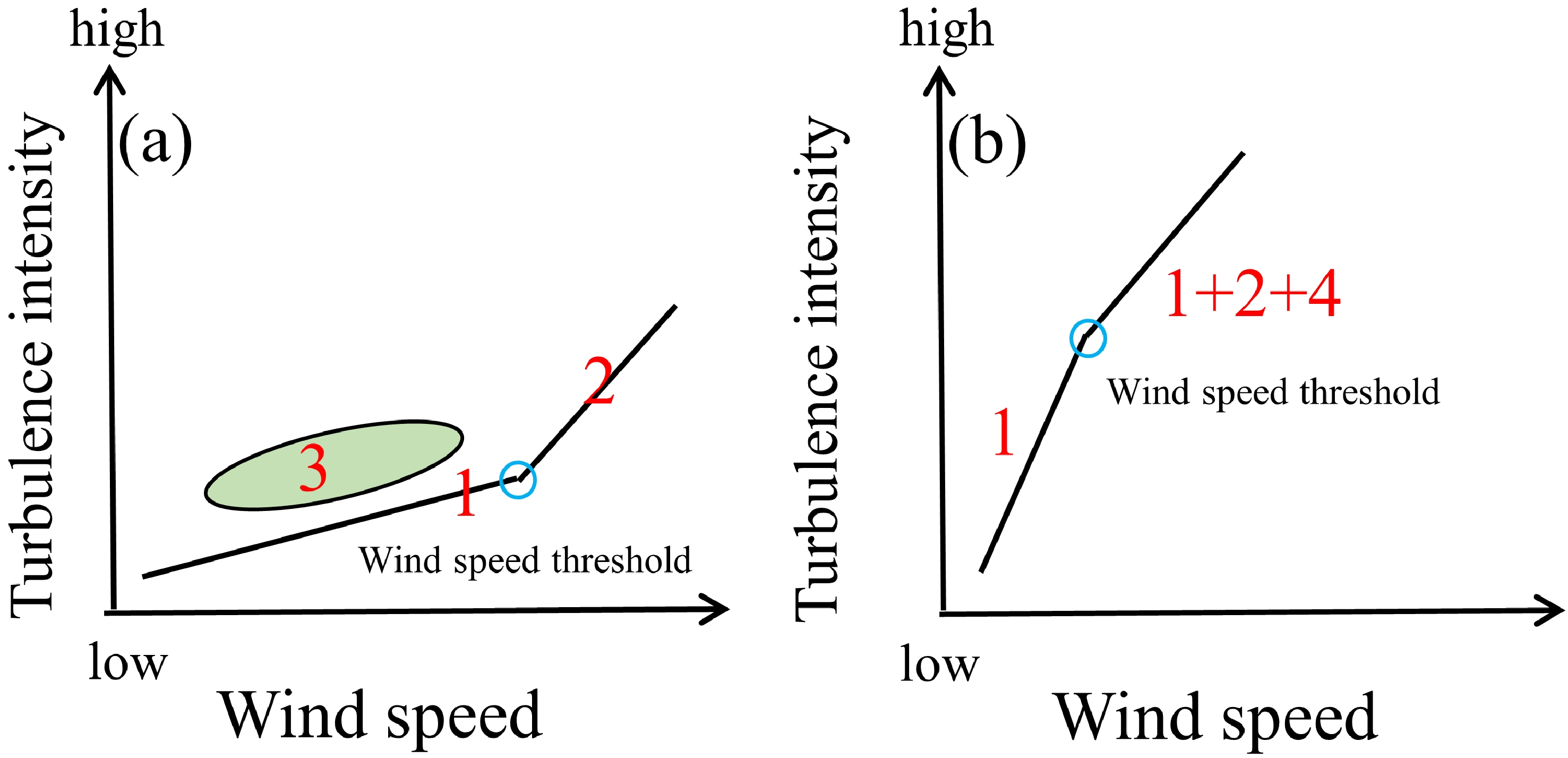
$(\overline{{u}^{'2}}+\overline{{v}^{{'}2}})/2$ and vertical TKE$\overline{{w}^{{'}2}}/2$ at (a) 15 m, (b) 47 m, (c) 80 m, (d) 140 m, (e) 200 m, and (f) 280 m. The red, green and blue circles represent three kinds of stable boundary layers according to the vertical profile of TKE: weak transport, upside-down and downside-up, respectively. The three patterns were classified according to the vertical profiles of TKE.Based on the above analysis, we can infer the schematic representation VTKE vs. V applicable to the UBL. For the layers above the UCL, or more accurately, the layers having little influence from the thermodynamic properties of the urban canopy, VTKE vs. V is consistent with the HOST theory proposed by Sun et al. (2012) based on the flat underlying surface (Fig. 8a). Local shear plays a leading role when V<VT (regime 1); strong turbulence is mainly driven by the bulk shear when V>VT (regime 2); and small wind speed accompanied by moderate turbulence intensity, i.e., upside-down structure (regime 3).
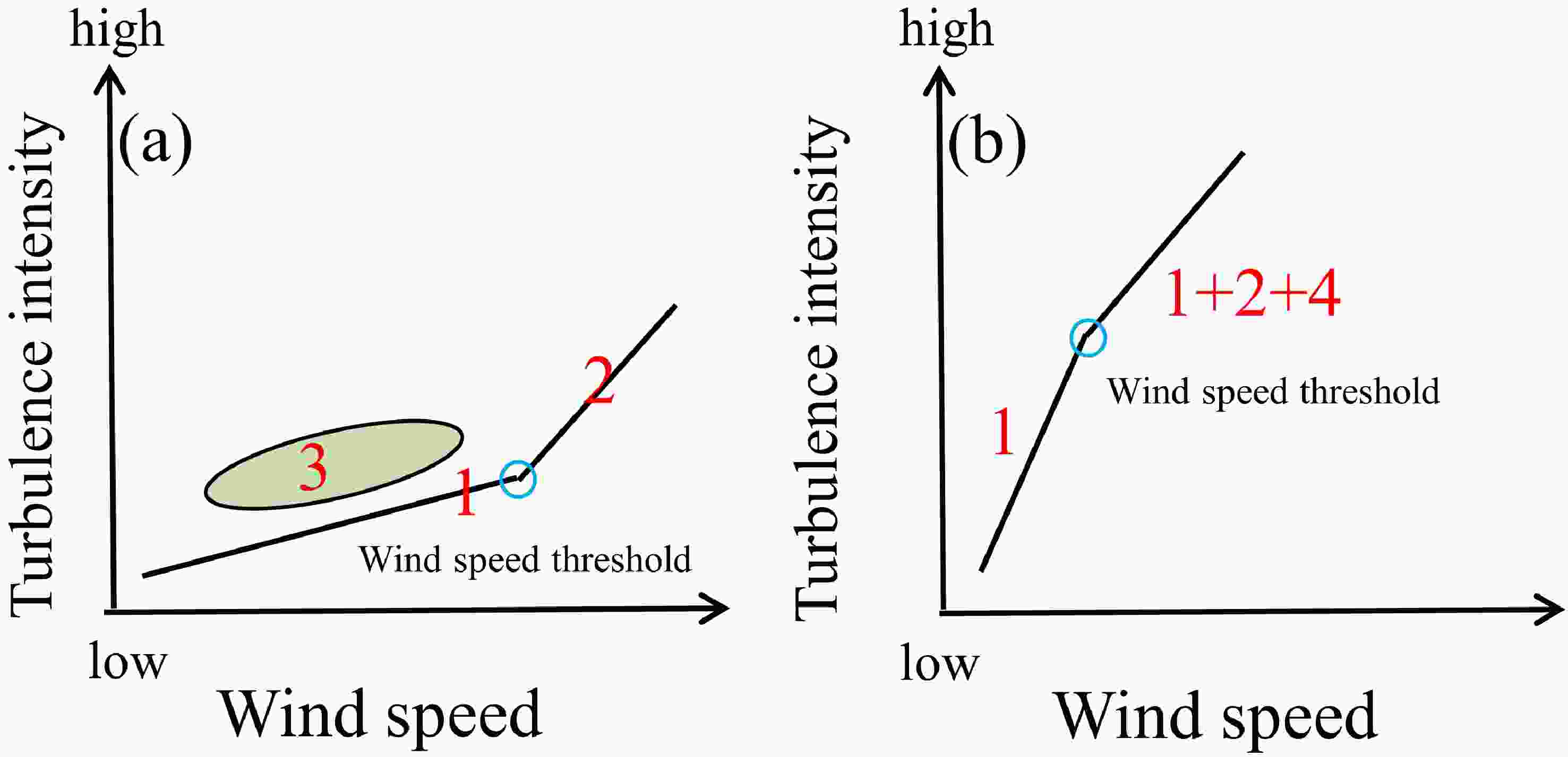
Figure 8. Schematic representation of the relationship between the turbulence strength VTKE and the wind speed V with the four turbulence regimes (regimes 1, 2, 3, and 4) for the Beijing 325-m meteorological tower, located at a typical city underlying surface. (a) 140 m, 200 m, and 280 m; and (b) 8 m, 15 m, 47 m, and 80 m. The urban canopy height of the observation site is estimated to be approximately 80 m. Turbulence in regime 1 is mainly generated by local instability. Turbulence in regime 2 is mainly generated by bulk shear. Turbulence in regime 3 is mainly generated by upside-down turbulence flows. Turbulence in regime 4 is generated by buoyancy turbulence flows.
The schematic representation in Fig. 8b is more appropriate for heights within the UCL. The UCL height near Beijing 325-m meteorological tower in this paper was approximately 47 m. Fig. 8b shows the characteristics of VTKE vs. V at 8, 15, 47 and 80 m. The influence of local wind shear in the canopy was strongest, and the relationship of VTKE vs. V was much closer when V<VT (regime 1). As for the strong turbulence activities when V>VT, the generation of strong turbulence is the result of a combination of local wind shear (regime 1), bulk shear (regime 2), and anthropogenic heat (regime 4).
-
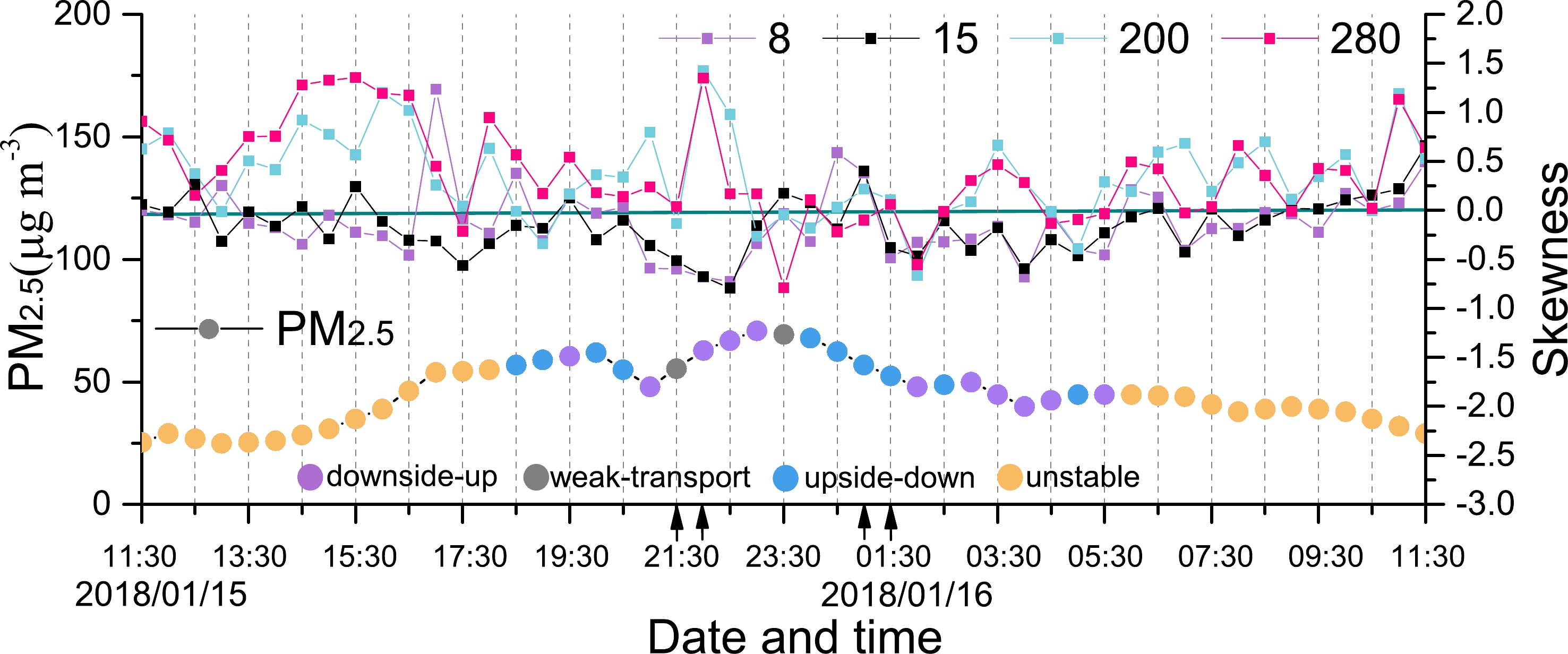
The current study investigated the relationship between different turbulence regimes and the evolution of the concentration of pollutants. Figure 9 shows the time series of the concentration of the ground PM2.5 at the OSCS station from 1130 LST Jan 15 to 1130 LST January 16 as well as the corresponding SBL types. Figure 9 also demonstrates the variation in skewness-w.
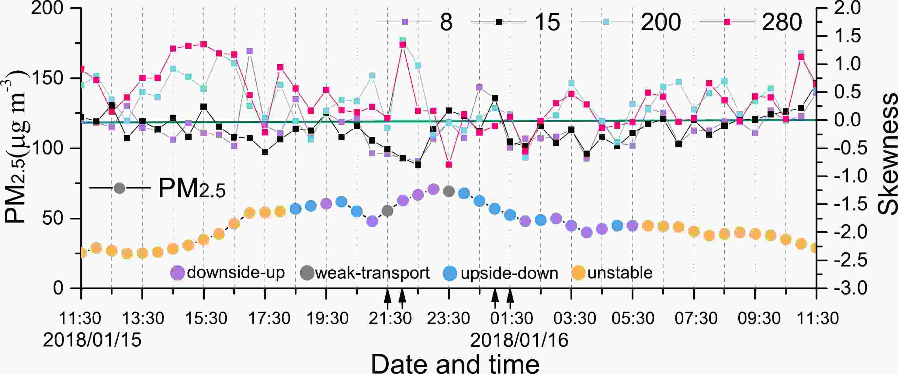
Figure 9. The time series of the skewness of the vertical velocity at 8 m, 15 m, 200 m and 280 m and the concentration of PM2.5 from 1130 LST on 15 January 2018 to 1130 LST on 16 January 2018. The variation process is marked by different circle colors, representing the different boundary layer structures.
We selected 8, 15, 200 and 280 m within the tower observation layer. Figure 9 shows that skewness-w had a stratification influence behavior. Specifically, the skewness-w values of 8 and 15 m in the lower layer tended to be negative, and the turbulence exchange process was mainly affected by the sweep process. By contrast, the skewness-w at the upper layers of 200 and 280 m remained positive, demonstrating that the turbulence exchange process was mainly dominated by the ejection process and that the diurnal variation in skewness-w was not significant.
Due to the occurrence of the upside-down structure, the positive skewness-w of 200 and 280 m in the upper layer gradually decreased and gradually approached the value of the lower layer or even decreased to a negative value, indicating that the turbulence exchange process in the upper layer gradually changed from ejection to sweep.
The relationship between the SBL structure and the concentration of pollutants was not very obvious, as shown in Fig. 9. Theoretically, weak-transport is regarded as favorable to the accumulation of pollutants. The sweep exchange process is more conducive to the removal of pollutants; therefore, the decreasing trend of the concentration of pollutants often correlates with the emergence of an upside-down structure.
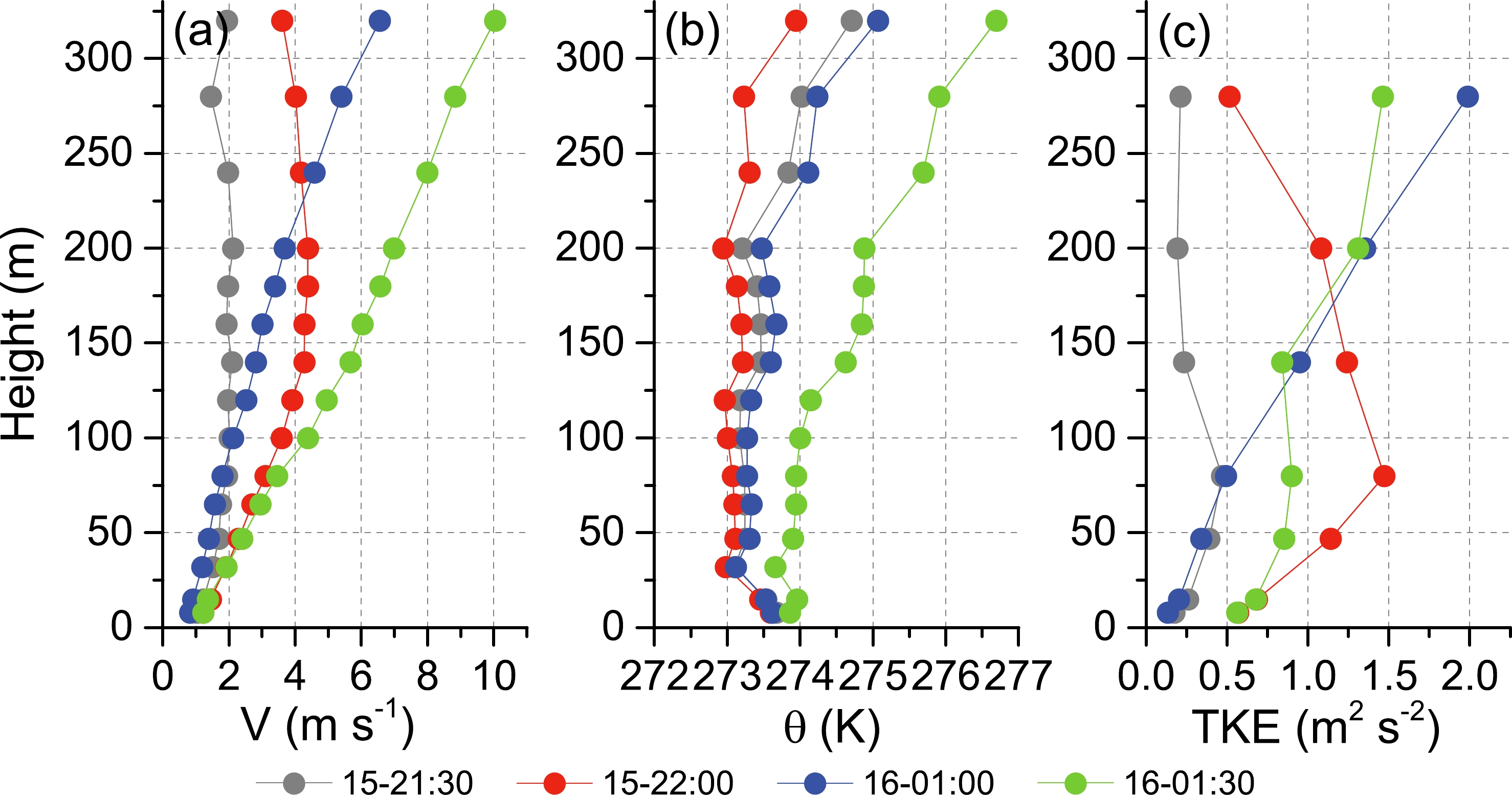
Figure 10 further shows the vertical distribution of V, potential temperature and TKE of the three SBLs: 2130 LST on Jan 15 was weak-transport, 2200 LST on Jan 15 was downside-up, and 0100 LST on Jan 16 and 0130 LST on Jan 16 were upside-down structures. From 2130 LST on 15 Jan to 0130 LST on 16 Jan, although the potential temperature near the ground was not the lowest, the stability of the lower atmosphere still deepened. For the wind profile, the V in the lower canopy was significantly reduced due to the blocking effects of the buildings within the UCL. The wind profile for the upside-down structure became more irregular and obviously did not conform to the logarithmic law.

Figure 10. Typical vertical profiles of wind speed (V), potential temperature and turbulence kinetic energy (TKE) at 2130 LST on 15 January 2018 for weak transport, 2200 LST on 15 January 2018 for downside-up, 0100 LST on 16 January 2018 and 0130 LST on 16 January 2018 for upside-down structures.
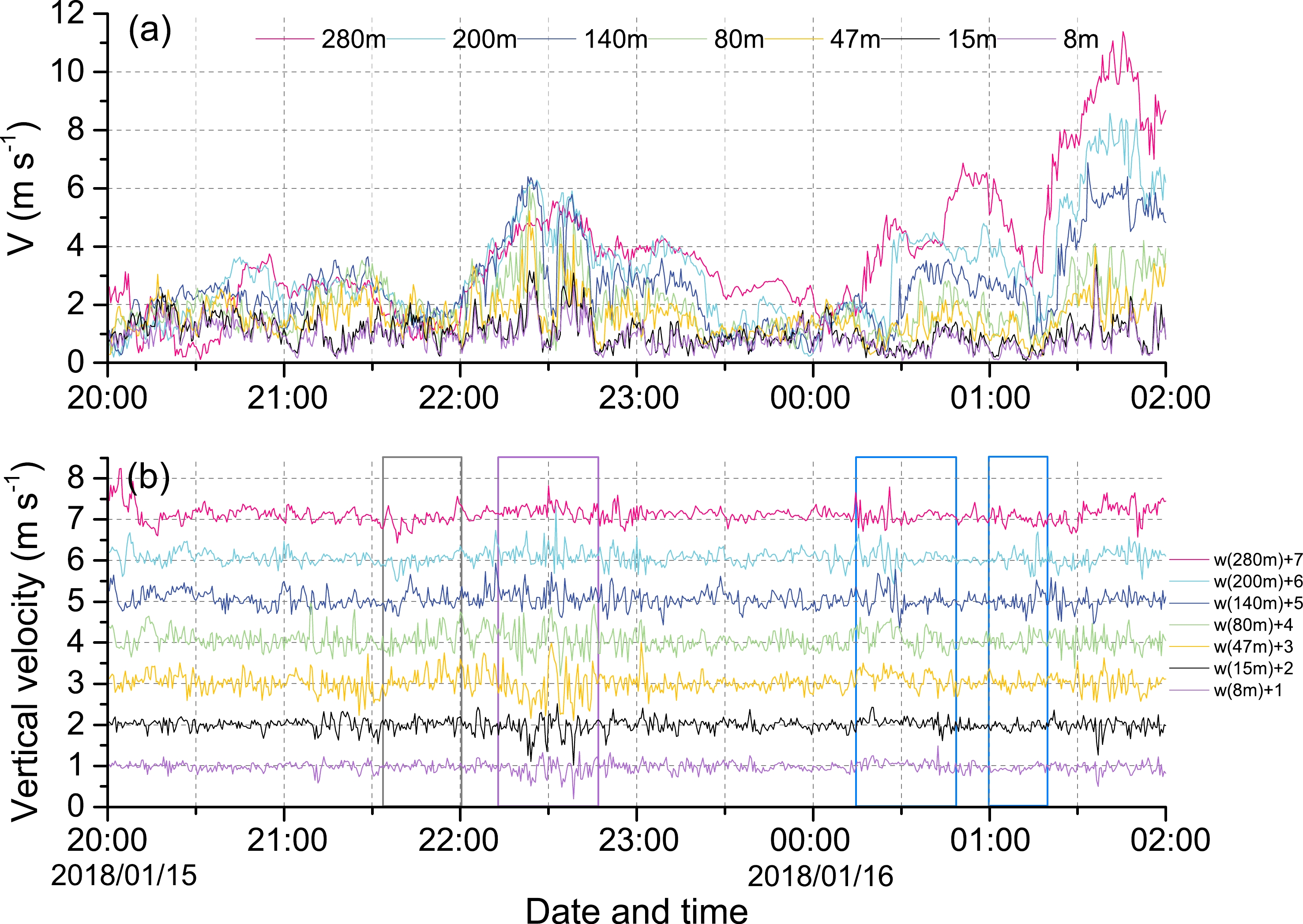
The evolution of V and vertical wind speed w clearly demonstrated the transformation between different turbulence regimes (Fig. 11). The data shown were the 30 s temporal average from sonic anemometers with a frequency of 10 Hz. From 2130 LST to 2200 LST on 15 Jan, the V of the whole tower layer became very small, almost less than 2 m s−1. The turbulence of the tower layer belonged to regime 1, and at this time, the concentration of ground PM2.5 gradually increased, and the skewness-w at 8 and 15 m gradually decreased (shown in Fig. 9). At approximately 2230 LST on 15 Jan, except for the relatively small V in the lower layer of the tower, V increased significantly, and V within the tower layer was relatively uniform. When V gradually increased, w also changed simultaneously, and the absolute value of the vertical velocity
$ \left|w\right| $ increased. The turbulence regime has mainly evolved into regime 2.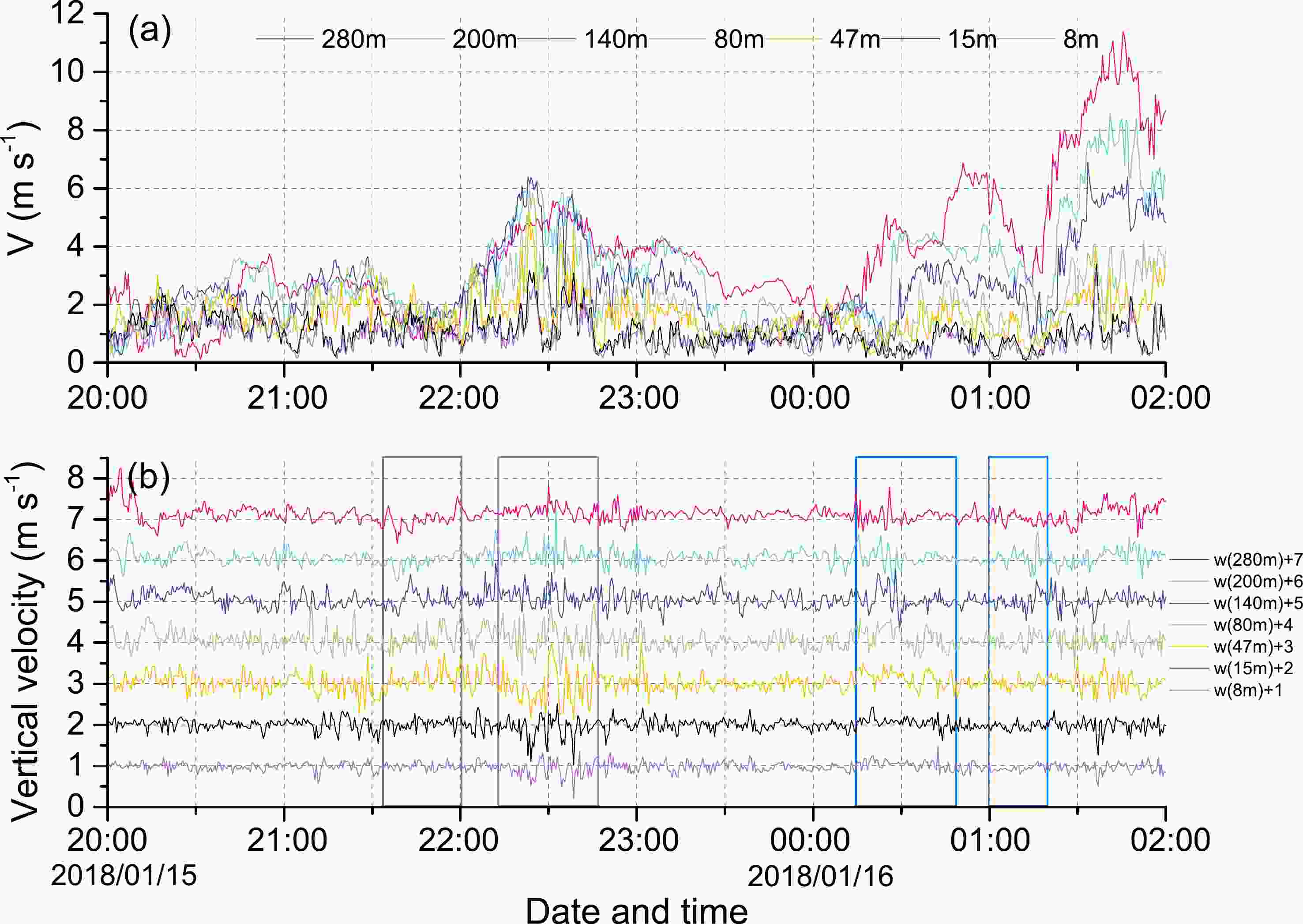
Figure 11. The time series of the wind speed V and the vertical velocity w for the seven observation levels from 2000 LST on 15 January 2018 to 0200 LST on 16 January 2018. For vertical velocity w starting from 15 m, the value is shifted by the amount shown to the right of each time series. The data shown are the 30 s temporal average from sonic anemometers with a frequency of 10 Hz.
Generally, the decrease in V, an increase in the variability of w with height, and negative value of the skewness-w indicated the downward transport of TKE (Mahrt and Vickers, 2002; Yus-Díez et al., 2019). At approximately 0030 LST on 16 Jan, the skewness-w at 280 m decreased, changing to a negative value, and the skewness-w at 15 m was also a negative value (Fig. 9). The variation amplitude in w increased with height (Fig. 11b), and this maximum w propagated downward to lower levels with time. However, at this time, the variation in the V of each layer changed sharply, and the upside-down structure in the UBL was affected by the UCL.
From 0100 LST to 0120 LST on 16 Jan, tower observation data show that V at 200 and 280 m decreased rapidly, and V in the lower layer did not change greatly; the variability of w at 80, 140, 200 and 280 m was significantly greater than that in the lower layers at 8, 15, and 47 m. The skewness-w at 280 m changed to a negative value. Although skewness-w was not negative at 200 m, its absolute value also decreased significantly. Figure 10 shows that within the tower layer at this time, TKE gradually increased with height, indicating an obvious upside-down structure.
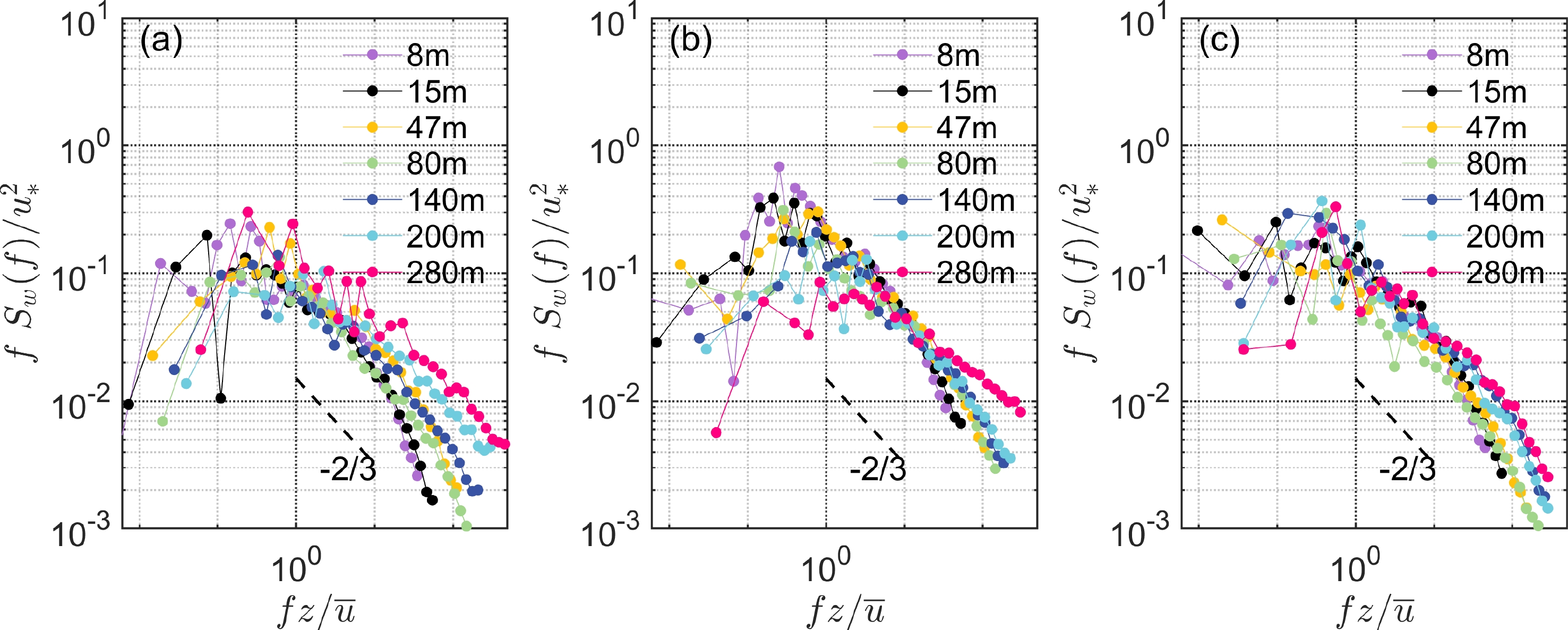
Figure 12 shows the power spectra of w at 2100 LST on 15 Jan 2018, 2200 LST on 15 Jan 2018 and 0000 LST on 16 Jan 2018, representing the power spectra distribution for weak-transport, downside-up and upside-down structures, respectively. The power spectra of w for three stages mainly satisfied the “–2/3” power law in the inertial subrange. At 2200 LST on 15 Jan 2018, when TKE was transmitted upward from the UCL during strong wind, the power spectra of w in the inertial subrange were more consistent. When an upside-down structure occurred (Fig. 12c), the spectral density at a low-frequency increased, suggesting the influence of the large-scale motions. However, overall, the w spectra had no prominent peak at lower frequencies, revealing that the large-scale motions were essentially horizontal near the ground (Li et al., 2007). Compared to that from flat terrain, the w spectrum showed an obvious power deficit at intermediate frequencies near the spectral peak, a feature that has been reported for spectra over complex terrain (Gallagher et al., 1988).

Figure 12. Power spectra of the w wind component at weak transport at 2100 LST on 15 January 2018 (a), downside-up at 2200 LST on 15 January 2018 (b), and upside-down at 0000 LST on 16 January 2018 (c). A 1-h data segment is used at each observation height in both panels.
We further analyzed the corresponding vertical distribution of the stability parameters of different SBLs (seen in Table 2). To make the results more obvious, stable (S), near-neutral (N) and unstable (U) refer to the z/Λ>0.1,
$ \left|z/\varLambda \right| $ <0.1, and z/Λ<–0.1 cases, respectively. The neutral cases occurred most frequently for downside-up because near-neutral stratification usually corresponded to windy days, and stronger winds were more often associated with neutral stratification. Weak-transport mostly corresponded to low wind days, and the occurrence probability of neutral stratification for weak-transport in each layer was smallest. The occurrence of stable stratification should be highest for weak transport, but this result was only available for the lower layer of the tower (8–47 m). The highest frequent stable stratification in the higher layer usually corresponded to the upside-down structure. The more stable stratification may lead to the decoupling between the lower layer and the layer above it; therefore, the mixing process between different layers was partially weakened. The momentum of the upper layer could not be transferred to the lower layer and then consumed, resulting in a relatively larger TKE in the upper layer.Height (m) 8 15 32 47 65 80 100 120 140 160 180 200 240 280 320 Meterological √ √ √ √ √ √ √ √ √ √ √ √ √ √ √ Turbulence √ √ √ √ √ √ √ Table 1. Instrument heights on the Beijing 325-m meteorological tower.
Height Downside-up Weak transport Upside-down S N U S N U S N U 8 m 35.6 62.2 2.2 72.4 16.1 11.5 62.1 31.8 6.1 15 m 39.8 57.0 3.2 70.7 14.2 15.1 62.2 27.5 10.3 47 m 29.0 57.6 13.4 51.7 8.1 40.2 47.9 30.2 21.9 80 m 29.0 52.1 18.9 44.0 8.5 47.5 50.1 26.6 23.3 140 m 38.4 30.1 31.5 46.2 3.2 50.6 56.0 15.7 28.3 200 m 61.4 14.2 24.4 53.5 2.0 44.5 70.0 7.0 23.0 280 m 63.7 10.3 26.0 52.4 1.7 45.9 67.3 7.3 25.4 Table 2. The distribution of the frequency (%) for stable (S, z/Λ>0.1), near-neutral (N,
$\left|z/\varLambda \right|$ <0.1) and unstable (U, z/Λ<–0.1) cases of the nighttime downside-up, upside-down, weak-transport cases from November 2017 to January 2018 observed by the 325-m tower. -
Because of the unique complex underlying surface of the UCL, such as significant roughness and anthropogenic heat, the thermodynamic properties of the UBL are therefore greatly modulated. The Beijing 325-m meteorological tower is located on a typical UUS. Various tall buildings, roads and vegetation covers around the tower exert strong disturbances on the surrounding air flows.
Based on meteorological tower data from Nov 2017 to Jan 2018, this study analyzed NSBL turbulence regimes over urban areas and calculated the relationship between VTKE and V applicable to the UBL. The results showed that for heights above the UCL (140, 200 and 280 m), the influence of the canopy was relatively small. The pattern of VTKE vs. V is consistent with the HOST theory proposed according to the flat area: a) regime 1 characterized by low turbulence intensity when V<VT, generated by local shear; b) regime 2 characterized by strong turbulence caused by bulk shear when V>VT; and c) regime 3 characterized by small V with moderate turbulence intensity, in which the turbulence was enhanced by sporadic upside-down turbulence. The upside-down structure had a higher downward transmission efficiency of the horizontal TKE.
For the height inside the canopy (8, 15, 47 and 80 m), these layers were strongly affected by the thermal-dynamic properties of the UCL. Weak turbulence in the UCL was strongly affected by local wind shear (regime 1) when V<VT, and the local wind shear was the most important determining factor for the variation in VTKE. When V>VT, local wind shear was still very important for the generation of turbulence. For strong turbulence regime when V>VT, the generation of strong turbulence is a result of a combination of local wind shear (regime 1), bulk shear (regime 2), and buoyancy turbulence (regime 4).
This study focused on the SBL at night and selected the cases when z/Λ>0. However, some thermal instability stratification (
$ \Delta \theta < 0 $ ) cases in the UBL were still observed when z/Λ>0 (negative kinematic heat flux$\overline{{w}^{{'}}{\theta }_{v}^{{'}}}$ ), demonstrating the emergence of counter gradient transportation of heat in the nighttime UBL. The heat was transmitted from the layer with low temperature to the layer with higher temperature. Moreover, strong turbulence within the UCL was usually accompanied by this thermally unstable stratification; therefore, the buoyancy turbulence also constituted the generation of strong turbulence within the UCL (regime 4). The thermal stratification was weakly related to the turbulence intensity when the small turbulence eddies were strongly correlated with the local shear. The turbulence generated by bulk shear was more likely to be affected by thermal stratification. Turbulence was partially suppressed with the stratification$ \Delta \theta $ >0.5.According to the vertical profiles of TKE, this study shows the typical vertical distribution of three different SBLs: downside-up, weak-transport, and upside-down. The transformation between different SBLs, turbulence regimes, and their relationships with the concentration of pollutants were also investigated by analyzing the evolution of V, vertical wind speed w, and skewness-w. The value of skewness-w at 200 and 280 m gradually decreased or even became negative, and the turbulence exchange process gradually changed from ejection to sweep when the upside-down structure occurred. The power spectra of w for three SBLs mainly satisfied the “–2/3” power law in the inertial subrange. When an upside-down structure occurred, the spectral density at a low-frequency increased. The w spectrum showed an obvious power deficit at intermediate frequencies near the spectral peak because of the influences of complex terrain.
When the TKE of the tower layer was less than 0.5 m2 s−2 and the vertical exchange of TKE was weak, it could be inferred that most of these cases displayed stable stratification. However, this conclusion was more applicable to the lower layer (8–80 m) of the tower. The stable stratification at 140–280 m mostly corresponded to the upside-down structure. This may be because the more stable stratification was easier to decouple between the higher and lower layers, the mixing process between different layers was thus reduced, and the momentum of the higher layer was therefore not greatly consumed, resulting in the larger TKE in the higher layer.
The results in this paper are helpful for deepening the understanding of the turbulence regimes and the turbulence structures over complex underlying surfaces and for providing more scientific improvements for the simulation of the UCL.
Acknowledgements. Many thanks to the anonymous reviewers, who provided useful suggestions to improve the quality of the manuscript. This work was supported by the National Natural Science Foundation of China (Grant No. 42105093 and 41975018); the China Postdoctoral Science Foundation (Grant No. 2020M670420) and the Special Research Assistant Project. The datasets generated and analyzed in this study are available from the corresponding author on reasonable request.
| Height (m) | |||||||||||||||
| 8 | 15 | 32 | 47 | 65 | 80 | 100 | 120 | 140 | 160 | 180 | 200 | 240 | 280 | 320 | |
| Meterological | √ | √ | √ | √ | √ | √ | √ | √ | √ | √ | √ | √ | √ | √ | √ |
| Turbulence | √ | √ | √ | √ | √ | √ | √ | ||||||||


 AAS Website
 AAS WeChat