


 DownLoad:


-
Land surface absorbs about 50% of incoming solar energy at the top of atmosphere and returns it back to the atmosphere as radiative energy, sensible heating, and latent heating (Trenberth et al., 2009). In addition, there are bidirectional exchanges of carbon, nitrogen, water, and other fundamental materials between land surface and the atmospheric boundary layer (Betts et al., 1996). In all these energy transfer and mass exchanging processes, land surface properties play key controlling roles.
Microwave Land Surface Emissivity (MLSE) is the ratio between microwave irradiance emitted from land surface to that from an ideal blackbody with the same thermodynamic temperature. It contains abundant information of soil texture, soil moisture, vegetation water content, vegetation vertical structure, surface roughness, etc. (Aires et al., 2001; Prigent et al., 2003). Therefore, MLSE has broad applications in satellite remote sensing of soil moisture (Jackson and Schmugge, 1991; Wigneron et al., 1995; Owe et al., 2001, 2008; Wigneron et al., 2017), evaluation of droughts and floods (Li and Min, 2013; Zhang and Jia, 2013; Liu et al., 2017a), wildfire risk assessment (Forkel et al., 2017; Fan et al., 2018; Forkel et al., 2019), monitoring the phenology of forests (Min and Lin, 2006a; Min et al., 2010; Jones et al., 2011; Li et al., 2020a), estimation of carbon uptake, gross primary production (GPP), and above ground biomass (AGB) (Wigneron et al., 1995; Liu et al., 2015; Brandt et al., 2018). In particular, MLSE is very sensitive to vegetation water content, making it a crucial indicator to infer potential changes of water status inside the vegetation canopy (Wang et al., 2019a, b; Li et al., 2020a). On the other hand, MLSE determines the upwelling microwave radiation at a given land surface temperature (LST), and thus provides the background signals for satellite physical-based retrieval of precipitation over land using passive microwave measurements (Ferraro et al., 2013; Randel et al., 2020). The uncertainty introduced by highly varied MLSE is the major factor holding back the progress of passive microwave remote sensing of precipitation over land (Prigent et al., 1997).
MLSE has been retrieved since the 1990s using measurements from series of passive microwave radiometers on board low earth orbit satellites. For instance, multiple studies have been conducted using measurements from Special Sensor Microwave Imagers (SSMI) (Prigent et al., 1997, 1998, 2006; Min and Lin, 2006b), Tropical Rainfall Measuring Mission (TRMM) Microwave Instrument (TMI) (Prigent et al., 2008), Advanced Microwave Sounding Units (AMSU) (Karbou et al., 2005), Microwave Humidity Sounder (MHS), and Advanced Microwave Scanning Radiometer - Earth Observing System (AMSR-E) (Min et al., 2010; Moncet et al., 2011a; Norouzi et al., 2011, 2012; Li et al., 2020a; Hu et al., 2021).
Microwave Radiation Imager (MWRI) is a fundamental instrument on board Chinese Fengyun (FY) series satellites including FY 3A (launched on 27 May 2008), 3B (launched on 4 November 2010), 3C (launched on 23 September 2013), and 3D (launched on 15 November 2017). The MWRI radiometer observes the Earth’s surface with a conically scanning microwave antenna from an Earth incidence angle (EIA) of 53.1°, with ascending and descending nominal equator crossing times (ECT) around 13:30 and 01:30 local time (LT). It measures brightness temperatures at both vertical and horizontal polarized frequencies centered at 10.65 GHz, 18.7 GHz, 23.8 GHz, 36.5 GHz, and 89.0 GHz (Yang et al., 2011b). The MWRI sensor plays a critical role in providing continuous measurements of the thermal microwave emission from land and ocean surfaces and information on various forms of water within the atmosphere, clouds, and surfaces.
MWRI brightness temperature (Zhang et al., 2019) has been widely used to retrieve many atmospheric and surface parameters such as soil moisture (Bao et al., 2014), snow depth (Jiang et al., 2014), liquid water path (Yang et al., 2012; Tang and Zou, 2017), and precipitation (Yang et al., 2012). Wu et al. (2019) retrieved microwave land surface emissivity over the Qinghai-Tibetan Plateau under clear sky conditions using FY-3B/MWRI Level 1 brightness temperatures.
Most previous studies related to satellite retrieval of MLSE focus on clear sky conditions. Limited studies have been done to retrieve MLSE under cloudy sky conditions. MLSE is a physical property that is intrinsically determined by surface characteristics, such as soil type, soil moisture, vegetation, and so on. From the perspective of microwave radiation transfer, it is largely determined by the dielectric constant of the mixed medium of air–soil–vegetation. Clouds can indirectly change MLSE by modulating the water content in this medium through evapotranspiration and photosynthesis processes (Min and Wang, 2008; Wang et al., 2021a, b, c). Generally, clouds can decrease the net solar radiation at the surface but increase the radiation use efficiency, and thus result in a nonlinear response of the water and carbon exchange rate between vegetation and the atmosphere. Consequently, this will lead to a change of vegetation inner water content. On the other hand, in the cloudy conditions shortly after rain events, MLSE is largely modified by the interception water over leaves, the increased soil moisture, and the inner vegetation water (Li and Min, 2013). Therefore, it is important to obtain and to investigate MLSE under cloudy sky conditions.
The key scientific questions here are: 1) how to get the cloud information (e.g., cloud water, cloud phase, cloud temperature, etc.) within the field of view of the microwave radiometer; and 2) how to subtract the contributions of those clouds from the upwelling brightness temperature at the top of atmosphere, so that the emission from land surface can be isolated from satellite-observed brightness temperature. To do this, cloud water properties in the path of the radiation transfer are required. Lin and Minnis (2000) utilized ground-based microwave radar observations of clouds to retrieve MLSE over the Southern Great Plains site on cloudy days. Min and Lin (2006b) applied this method to a midlatitude forest site in the northeastern United States. Min et al. (2010) and Li and Min (2013) combined Tb (brightness temperature) measurements from AMSR-E and the quasi-simultaneous retrieval of cloud properties from MODIS on the same satellite, Aqua, to obtain MLSE under cloudy sky areas. Baordo and Geer (2016) retrieved MLSE from SSM/I frequencies under cloudy conditions using an ECMWF reanalysis dataset of cloud properties as input. Based on the sensitivity tests in Hu et al. (2021), a perturbation of 300 g m–2 cloud water path only leads to less than 1% errors in MLSE retrievals at multiple frequencies. Therefore, the potential errors of satellite-retrieved cloud properties will only cause very limited uncertainties in MLSE retrieval. For MWRI, the quasi-simultaneous retrieval of cloud properties from visible and infrared sensors on the same satellite are still under development. In this study, we overcame this difficulty by using cloud properties derived from Advanced Himawari Imager (AHI) observations. The AHI is on board the Japanese Meteorological Agency (JMA) new-generation geostationary satellite, Himawari-8 (Bessho et al., 2016), launched into geosynchronous orbit around 140°E on 17 October 2014. The AHI level 2 cloud product (L2CLP) (Letu et al., 2019, 2020) retrieved from full disk measurements in the visible, shortwave infrared, and thermal infrared bands provides cloud top temperature (CTT), cloud effective radius (CER), cloud optical thickness (COT), quality assurance (QA) flags, etc. at 10-minute intervals and 5-km spatial resolution. Although there is still a small difference between the FY overpass time and the Himawari-8 AHI observing time, it provides the closest feasible observations of clouds in each footprint of MWRI over China.
In this application study, we adopt the general concept of the MLSE retrieval algorithm in Li et al. (2020a) and Hu et al. (2021) to process FY3B MWRI recalibrated brightness temperature combined with Himawari-8 AHI cloud retrievals. The major objective of this study is to introduce the structure of the algorithm and the retrieval process, and to show the main features of spatial and temporal distribution of MLSE over China under both clear and cloudy conditions. Detailed analyses of MLSE for particular regions and/or land cover types will be conducted in follow-up studies. Since there is no ground truth of MLSE, we indirectly evaluate the MWRI-based MLSE with two other AMSR-E MLSE products (Moncet et al., 2011a; Norouzi et al., 2011).
The description of the methods and the associated datasets are given in section 2. Then, the spatial distribution and temporal variations of MLSE in China and the inter-comparison studies between our results and multiple existing similar products (clear conditions only) are shown in section 3. Finally, we conclude the paper with a discussion and a summary in sections 4 and 5, respectively.
-
In the study, the FY-3B MWRI (Table 1) Level 1 recalibrated swath brightness temperatures (ascending orbits) were obtained from the National Satellite Meteorological Centre for 7 July 2015 through 30 June 2019. The spatial resolution varies between frequencies, and the instantaneous field of view (IFOV) sizes range from 51 km × 85 km at 10.65 GHz to 9 km × 15 km at 89.0 GHz. The historic MWRI raw data were generated into the fundamental climate data record (FCDR) with the latest preprocessing algorithms; the dataset underwent careful corrections in terms of geolocation errors (Tang et al., 2016; Li et al., 2020b; Liu et al., 2021) and issues of intrusion of the hot reflector, which was not accurately estimated in the prelaunch calibration process and resulted in a slight difference between the ascending and descending orbits (Xie et al., 2019). In addition, the MWRI data went through series of space-based cross-calibrations with SSMIS and TMI (Zhang et al., 2019), and, as is reported, most of the biases are within 1–2 K. The cross-calibrations of MWRI with AMSR-E and AMSR2 were conducted using the double difference method on the overlapped records (Du et al., 2014; Wu et al., 2020).
Frequencies (GHz) 6.925 10.65 18.7 23.8 36.5 89.0 MWRI sensitivity (K) − 0.5 0.5 0.5 0.5 0.8 AMSR-E sensitivity (K) 0.3 0.6 0.6 0.6 0.6 1.1 Table 1. The sensitivities of FY-3B MWRI and AMSR-E.
Himawari-8 AHI identifies sky conditions (clear or cloudy) by utilizing a cloud screening algorithm (Ishida and Nakajima, 2009) on the AHI L1B data and determines the cloud phase according to the brightness temperature (Tb) at different IR bands and their differences (Baum et al., 2000). In the AHI L2CLP cloud product, QA flags use two-bit values to provide information on the cloud retrieval quality confidence, cloud mask confidence level, cloud retrieval phase flag, and so on. Cloud retrieval phase flags were identified as “clear”, “liquid”, “mixed or uncertain”, or “ice”. The measurements covered the majority of China with a nominal coverage of 60°S–60°N, 80°E–160°W.
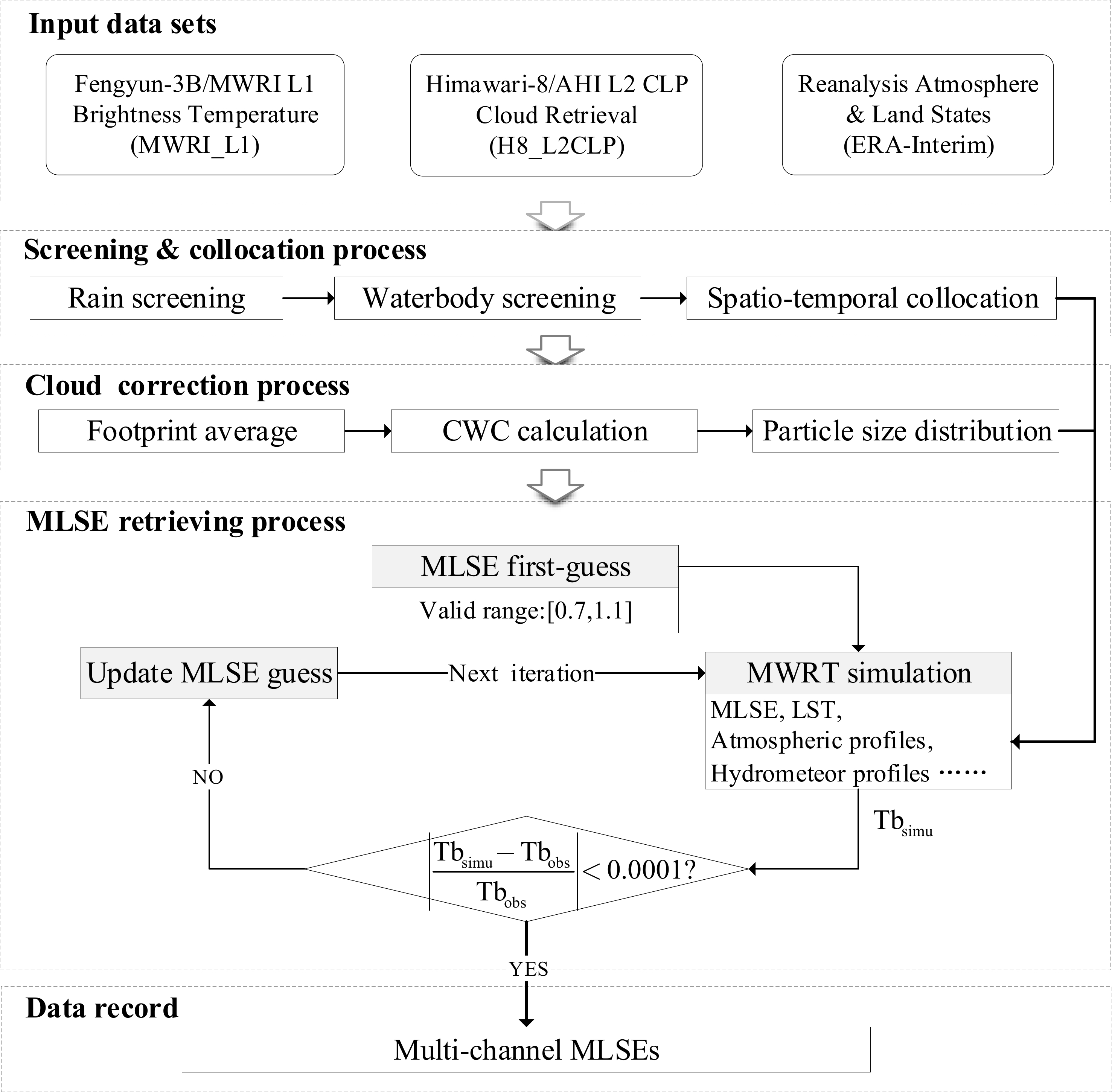
As shown in Fig. 1, we used a Microwave Radiative Transfer (MWRT) model (Liu, 1998) to simulate the upwelling microwave brightness temperature at the top of atmosphere (TOA) measured by satellite. The model is a four-stream radiative transfer model calculating Tbs for plane-parallel atmosphere using surface-, atmospheric-, and precipitation-related variables. It has been widely used in numerous studies (Liu, 2004; Noh et al., 2006, 2009; Okamoto et al., 2008; Aonashi et al., 2009a, b; Fujii et al., 2009; Shige et al., 2009, 2013; Wang et al., 2009, 2019a; Taniguchi et al., 2013; Kim et al., 2015; Jeoung et al., 2020; Kubota et al., 2020; Wu et al., 2020) for over 20 years and is actively being updated with new features. It is also used to calculate microwave single-scattering properties for non-spherical ice particles (Liu, 2004, 2008) as well as to retrieve snowfall (Noh et al., 2006, 2009; Liu, 2020). In the model, the contributions from land surface emission, the attenuation from atmospheric oxygen and water vapor, and the emission and scattering from cloud droplets were all included. Those fundamental inputs were derived from multiple data sources, including microwave measurements from the FY-3B MWRI, the observations and retrievals from visible and infrared sensors on the geostationary Himawari-8 satellite AHI, and the land surface temperature, the profiles of atmospheric temperature, water vapor, and geopotential height from ERA-Interim atmospheric reanalysis datasets (Berrisford et al., 2011). All pixels with Himawari-8-retrieved cloud water path over 300 g m–2 were assumed raining and were excluded from the MLSE retrieval process.
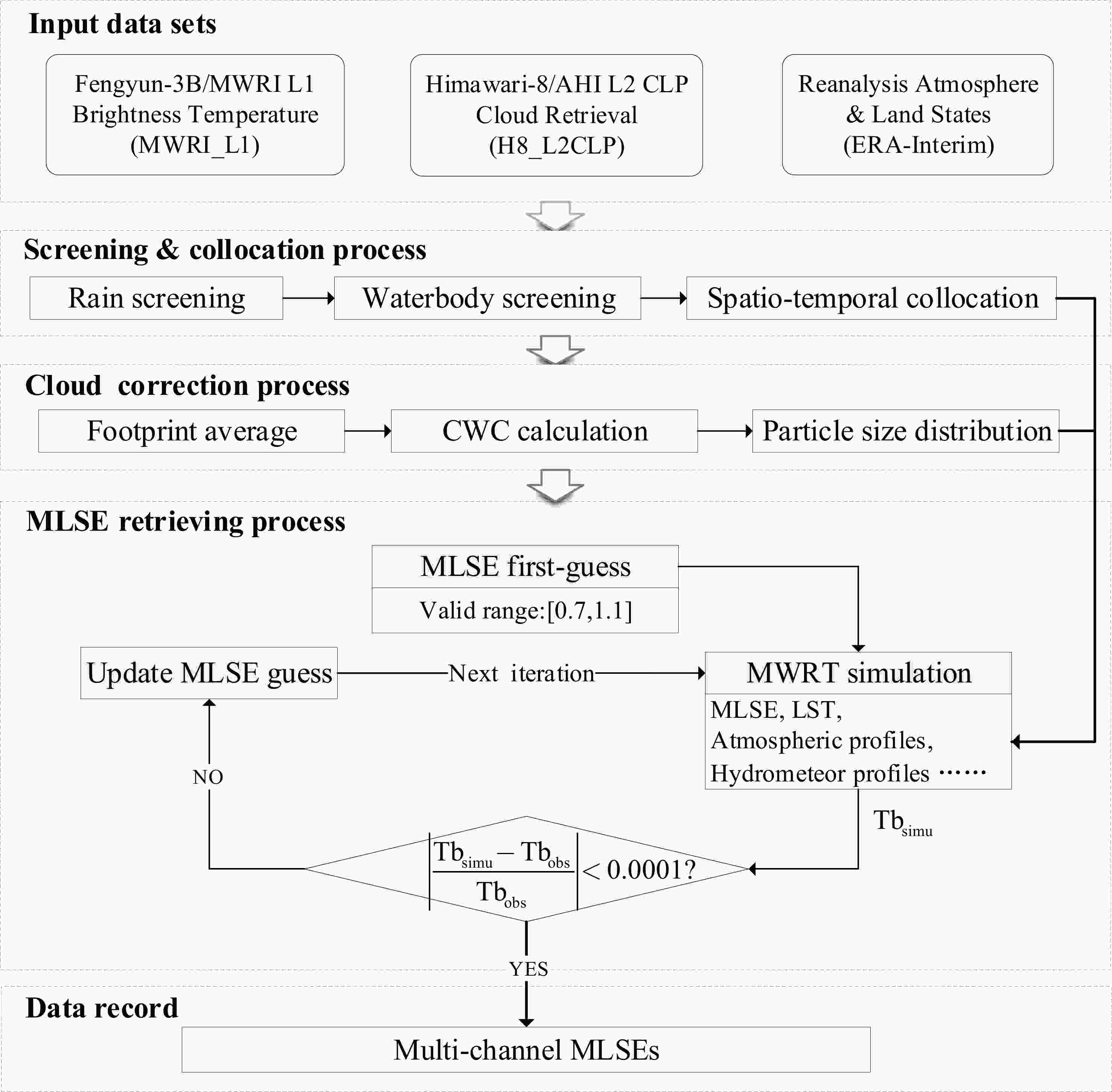
Figure 1. Flowchart of the FY-3B MWRI MLSE retrieval process.
In this study, we carefully considered the cloud contributions to TOA Tbs by using fused Himawari-8-retrieved cloud properties. Analogous to the work in Han et al. (2016), we collocated the high-resolution AHI cloud observations to the large MWRI footprint with the method of arithmetic mean. When collocating AHI cloud properties and MWRI observations, differences in footprint sizes at different MWRI channels were considered so that the high-resolution AHI clouds were averaged inside the corresponding footprint of certain MWRI channels individually. When fusing the ERA-interim atmospheric profiles and land skin temperature with MWRI, two 6-h ERA estimates that temporally bracket the MWRI overpassing time and spatially encompass from the nearest grid to the center of the MWRI footprint are collocated. Cloud water path (CWP) was derived from COT and CER with
$ \mathrm{C}\mathrm{W}\mathrm{P}=2/3\mathrm{C}\mathrm{O}\mathrm{T}{\rho }_{\mathrm{w}}\mathrm{C}\mathrm{E}\mathrm{R} $ for liquid phase and$ \mathrm{C}\mathrm{W}\mathrm{P}={\mathrm{C}\mathrm{O}\mathrm{T}}^{1/0.84}/0.065 $ for ice phase, where$ {\rho }_{\mathrm{w}} $ is the density of pure water. The optical and infrared observations of Himawari-8 did not provide vertical information on cloud properties. Therefore, we assumed a single-layer cloud located at the ERA-interim atmospheric profiles layer determined by CTT. Then, the cloud water content (CWC) of different cloud phases was calculated by dividing the derived CWP with the thickness of the determined cloud layer. In Liu’s (1998) MWRT model, cloud water and cloud ice were modeled as spherical particles; both liquid and ice phase droplets were assumed following the general three-parameter gamma particle size distribution:$ N\left(D\right)={N}_{0}{D}^{\mu }{e}^{-\lambda D} $ . For liquid phase, λ was set to$ 3\times {10}^{5} $ and μ = 2; for ice phase, λ was set to$ 2.55\times {10}^{3} $ and μ = 0 according to Heymsfield et al. (2002). The$ {N}_{0} $ was derived with the input CWC and specified λ and μ. The mixed-phase cloud water was treated as half liquid and half ice phases, and the two different halves were processed individually. The dielectric constants of liquid water and ice water were based on Lieb et al. (1991) and Mätzler (2006).Based on the above cloud configuration, the absorption and scattering coefficients of cloud particles were calculated using Mie theory in the microwave radiative transfer model. Therefore, for given TOA Tbs over a cloudy pixel, the contribution from clouds could be quantified. After further calculating the contributions from water vapor and oxygen, the upwelling Tbs at land surface could be derived. Then, the retrieval algorithm iteratively adjusted the value of MLSEs until the simulated TOA Tb matched the real satellite measurements.
As shown in Fig. 1, there are three main steps throughout the retrieval algorithm. First, multisource datasets were collocated on a spatiotemporal basis and by screening rainy/water/ocean pixels. A threshold of 0°C was set for the surface skin temperature to roughly screen out surface snow/frozen pixels. Second, AHI cloud observations in the MWRI footprints were converted to associated parameters required in the MWRT model. Thirdly, multichannel MLSEs were retrieved using the iterative process described in Fig. 1.
This retrieval process is independent for each FY-3B MWRI sample and channel. The final product covers the majority of China and parts of neighboring countries. Temporally, it spans from 1 July 2015 to 30 June 2019.
For comparing purposes, we compared our MLSE retrievals with the previous MLSE products derived from Aqua AMSR-E observations to assess the product under cloud-free conditions. Norouzi et al. (2011) built an MLSE product with frequencies ranging from 6.9 GHz to 89 GHz (Norouzi_MLSE) under cloud-free conditions. Moncet et al. (2011a) derived an emissivity product dataset (Moncet_MLSE) with frequencies above 10.65 GHz. The primary input data sources for retrieving MLSE are listed in Table 2. It should be mentioned that the two AMSR-E MLSE products represent the land surface properties during 2002 to 2010, while our MLSE is for 2015–19. The land use and land changes during those years will certainly introduce differences into the MLSEs.
Product MWRI_MLSE
(clear & cloudy sky)Norouzi_MLSE
(clear sky only)Moncet_MLSE
(clear sky only)Duration 20150701–20190630 20020701–20080630 20030101–20031231 Tb FY-3B MWRI AMSR-E L2A AMSR-E L2A Atmospheric profiles ECMWF/ERA-Interim ISCCP/TOVS NCEP/GDAS LST ECMWF/ERA-Interim ISCCP-DX MODIS LST Cloud flag Himawari-8/AHI L2CLP ISCCP-DX MYD06_L2 Cloud properties Himawari-8/AHI L2CLP − − Table 2. Data sources of the three MLSE products discussed in this study.
In addition, the MODIS/Aqua Vegetation Indices Monthly L3 Global 0.05Deg CMG (MYD13C2) dataset (Didan, 2015) was adopted to provide normalized difference vegetation index (NDVI) information on a monthly basis. In our analysis of the correlation between monthly MLSE and surface precipitation, daily rainfall estimation was taken from 1°
$ \times $ 1° Global Precipitation Climatology Project (GPCP) Climate Data Record (CDR), Version 1.3 (Daily) (Adler et al., 2017). MODIS/Aqua Snow Cover Monthly L3 Global 0.05Deg CMG (MYD10CM), Version 6 (Hall and Riggs, 2016) was obtained to provide the surface snow cover extent. -
Figure 2 shows an example of instantaneous MLSE retrieval on 26 July 2018 in the study area. Because the horizontal polarized (H-pol) MLSE is more sensitive to the surface changes in soil and vegetation water content (Prigent et al., 2006), we will primarily focus on horizontal polarizations in the following sections.

Figure 2. FY-3B MWRI-based instantaneous retrievals of MLSE (horizontal polarizations) at (a) 10.65 GHz,(b) 18.7 GHz, and (c) 36.5 GHz along with (d) cloud water path (CWP) retrieved from quasi-simultaneous observations from Himawari-8 AHI on 26 July 2018.
Of the selected study area, Fengyun-3B MWRI observed 69.7% of the land area, of which 66.3% was covered by clouds. In the MWRI-observed area, we successfully retrieved MLSEs in 86.7% area under both clear sky conditions and cloudy sky conditions. If we exclude all cloudy pixels, as previous algorithms did, we could only retrieve MLSE for 20.4% of the observed area. It should be noted that the radiative effect from clouds is not linearly proportional to the cloud fraction. And for a given cloud fraction, different types of clouds (cirrus, deep convective clouds, etc.) can make very different impacts on the MW radiative transfer.
By comparing the spatial distribution of retrieved MLSE and cloud water path (CWP, Fig. 2e), we can see a continuous and smooth transition of MLSE values from non-raining cloud-covered areas to cloud-free areas, indicating that the contribution of clouds is successfully removed from the retrieval algorithm.
From the probability distribution function (PDF) of retrieved MLSE (Fig. 3), we can see most of the values fall in the dynamic range of 0.7–1.0, except for a few samples at vertical polarizations of 18.7 GHz and 36.5 GHz, which result from random errors. It indicates most of our MLSE retrievals are at least reasonable. Generally, the PDF of MLSEs at lower frequencies are more at the low end than those at higher frequencies. This is consistent with our understanding about the frequency dependence of MLSE.

Figure 3. The probability distribution function (PDF, %) of retrieved MLSEs for 27 July 2018.
-
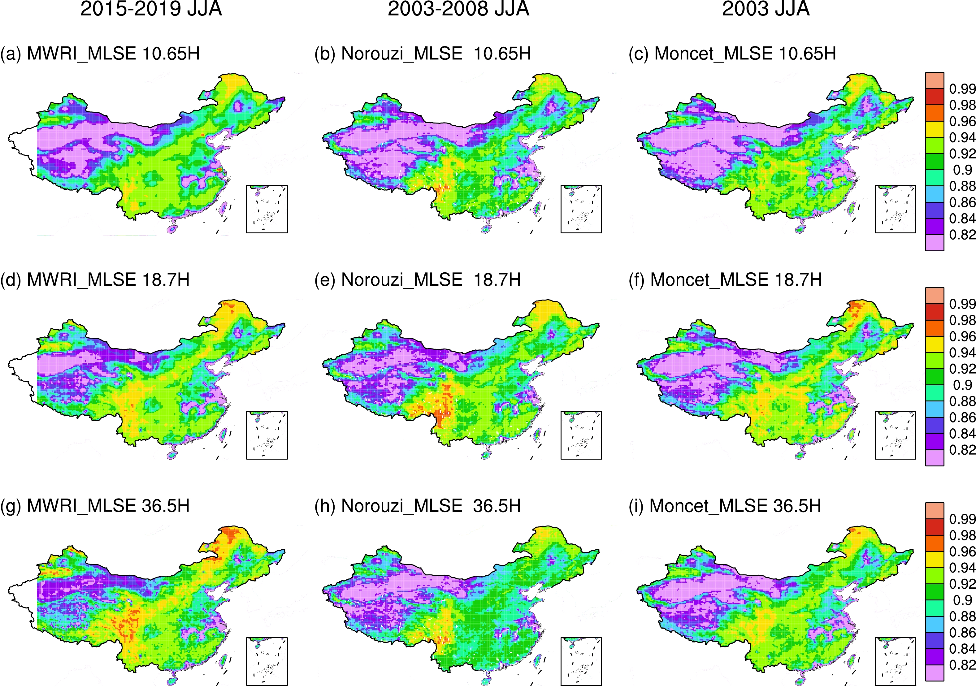
The spatial distributions of FY3B-MWRI MLSE at three frequencies (10.65 GHz, 18.7 GHz, and 36.5 GHz, horizontal polarization) for multiple-year-mean Summer (JJA) and Winter (DJF) are shown in Figs. 4 and 5. The associated results from Aqua AMSR-E Norouzi_MLSE (Norouzi et al., 2011) and Moncet_MLSE (Moncet et al., 2011a) are also shown. It should be noted that FY-3B MWRI and Aqua AMSR-E operated in different years. Due to the limitation of Himawari-8’s coverage, the FY3B-MWRI MLSE to the west of 80oE was not retrieved.
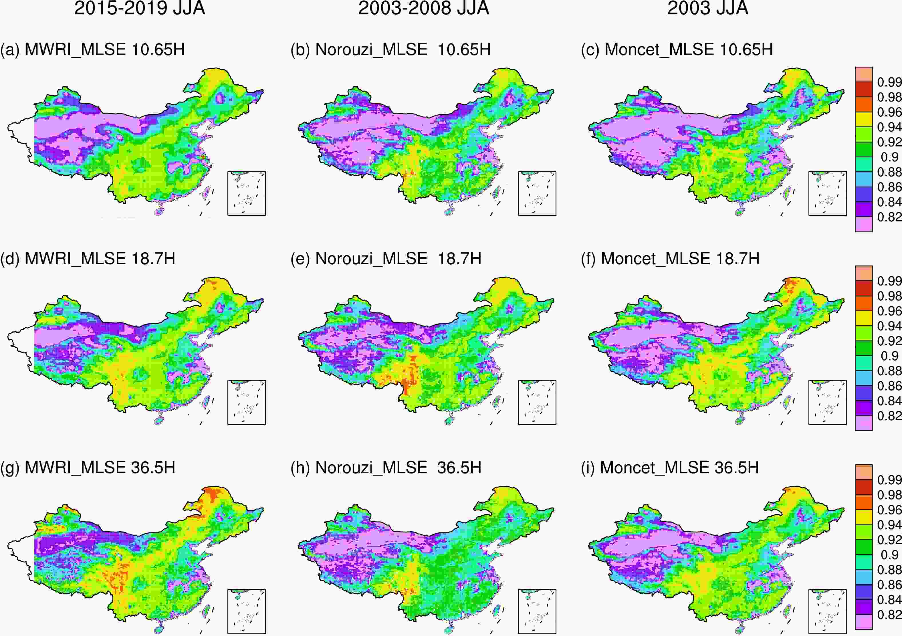
Figure 4. Spatial distributions of MLSEs derived from (a, d, g) FY-3B MWRI_MLSE (2015–19 JJA); (b, e, h) Aqua AMSR-E Norouzi_MLSE (2003–08, JJA), and (c, f, i) Aqua AMSR-E Moncet_MLSE (2003 JJA).
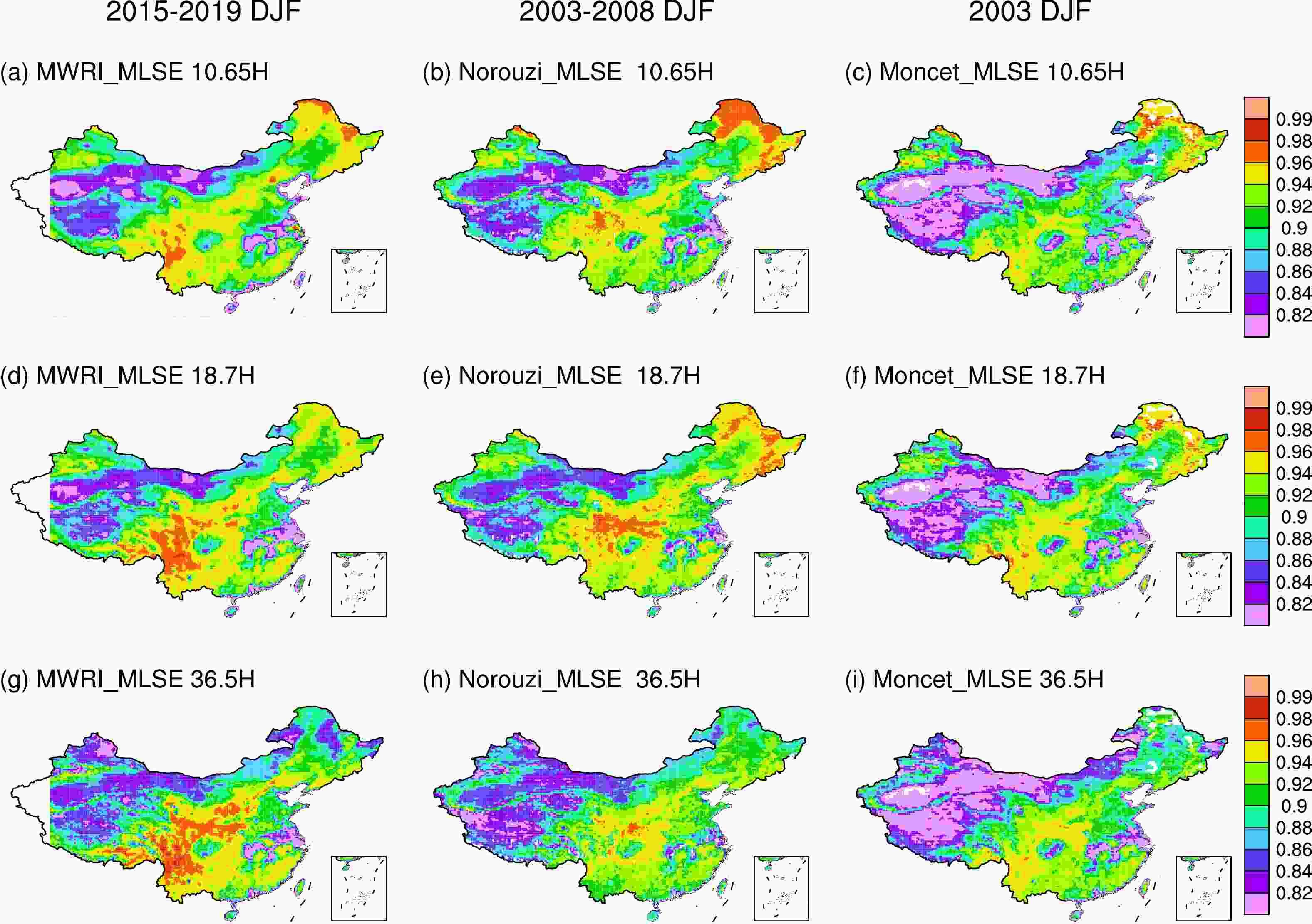
Figure 5. Same as Fig. 4, but for winter (DJF).
In summer (Fig. 4), our results show that the spatial distributions in China of MLSE for multiple channels are generally high in the southeast vegetated area and low in the northwest barren, or sparsely vegetated, area. The maximum values of MLSEs (particularly for 18.7 GHz and 36.5 GHz) are located in the southwest–northeast oriented belt area which is composed of the Qinling-Taihang Mountains and the eastern edge of the Qinghai-Tibet Plateau, which is also the dividing belt between high and low MLSE in China. Very low MLSEs (e.g., 0.8–0.86) are seen in Xinjiang (e.g., the Taklimakan Desert), western Inner Mongolia, and the Yangtze River delta. In southeastern China, there are still high spatial variations of MLSE with moderate values in vegetated areas and low values in river basins, coastal areas, and croplands, such as the Yangtze River basin, Sichuan basin, and northeast plain. In terms of frequency dependence, MLSEs generally increase with increasing frequency. However, in densely vegetated areas, such as forests in the southeast coastal and northeastern areas of China, MLSE at a lower frequency (e.g., 18.7 GHz) may be larger than that at a higher frequency (e.g., 36.5 GHz). This is consistent with the results in Min and Lin (2006b), Min et al. (2010), and Li and Min (2013).
In winter (Fig. 5), the spatial patterns of the three MLSE products are generally consistent. Previous studies have shown MLSE at low (high) frequencies over mountains and high-latitude areas increases (decreases) due to the snow cover effect (Prigent et al., 2006; Ferraro et al., 2013). The MLSE over the southern forest area also increases a little in winter. The seasonal variations of MLSE are further studied in the following section.
Relatively large discrepancies are found between the MLSE products in southwestern China, where the high values of this study’s MLSE are mainly located to the west and south of the Sichuan Basin; the high values of Norouzi_MLSE are more to the north and closer to Lanzhou; the Moncet_MLSE exhibits moderate values in southwestern China. These discrepancies of pattern and magnitude are mainly due to the use of different land surface temperature sources, which are significantly different in winter in this region. Overestimations are found in ISCCP skin temperatures (used by Norouzi et al., 2011) compared to those of ERA (used by this study) in these two regions. ISCCP daytime skin temperatures can be +5.0 K higher than MODIS in July, and there are areas with differences as large as 25 K (Moncet et al., 2011b). Although it is hard to tell which one is more biased, ERA represents the full range of weather conditions, whereas ISCCP and MODIS will miss cloudy samples. Additionally, the spread of snow cover in the high latitude regions in winter adds to this difference, since the snow is not completely removed from our retrieval. As for the high values in the Qinling-Taihang Mountains, as a common feature in all three products, the surface roughness and relief effect play main roles.
Despite a significant difference of observing years, the spatial patterns of FY3B-MWRI MLSE are highly consistent with Aqua AMSR-E Norouzi_MLSE and Moncet_MLSE. Detailed statistics of the correlation coefficient, root-mean-square error (RMSE), mean bias (MB), and mean absolute error (MAE) are shown in Table 3. As shown in Table 3, the spatial correlation coefficients between MWRI MLSE and the two AMSR-E MLSEs are 0.87–0.92 for horizontal polarizations and 0.67–0.83 for vertical polarizations in summer. The RMSEs are 0.016–0.022, and the MBs are –0.001–0.024, which are close to the differences between model-simulated MLSE and satellite retrievals reported by Prigent et al. (2015).
Frequency (GHz)/Polarization MWRI vs. Norouzi MWRI vs. Moncet Samples R RMSE MB MAE Samples R RMSE MB MAE 10.65H 15028 0.917 0.020 0.007 0.015 15348 0.904 0.022 0.015 0.021 18.7H 15028 0.920 0.019 0.002 0.013 15348 0.922 0.019 0.010 0.018 36.5H 15028 0.867 0.022 0.021 0.026 15348 0.898 0.020 0.020 0.023 10.65V 15043 0.748 0.016 0.005 0.012 15388 0.828 0.016 0.010 0.014 18.7V 15043 0.726 0.017 −0.001 0.012 15388 0.825 0.016 0.001 0.013 36.5V 15043 0.669 0.018 0.024 0.027 15388 0.808 0.017 0.016 0.019 Table 3. The statistical metrics of the intercomparison between MWRI MLSE and two AMSR-E-based MLSEs.
The high consistency between our MLSE and the two selected AMSR-E-based MLSEs indicates that the changes of land surface radiative properties during 2002 to 2019 are slow. It also demonstrates the measurements of Tb, including its calibration and validation by FY-3B MWRI, are reliable, and the retrieval algorithm developed in this study works well.
-
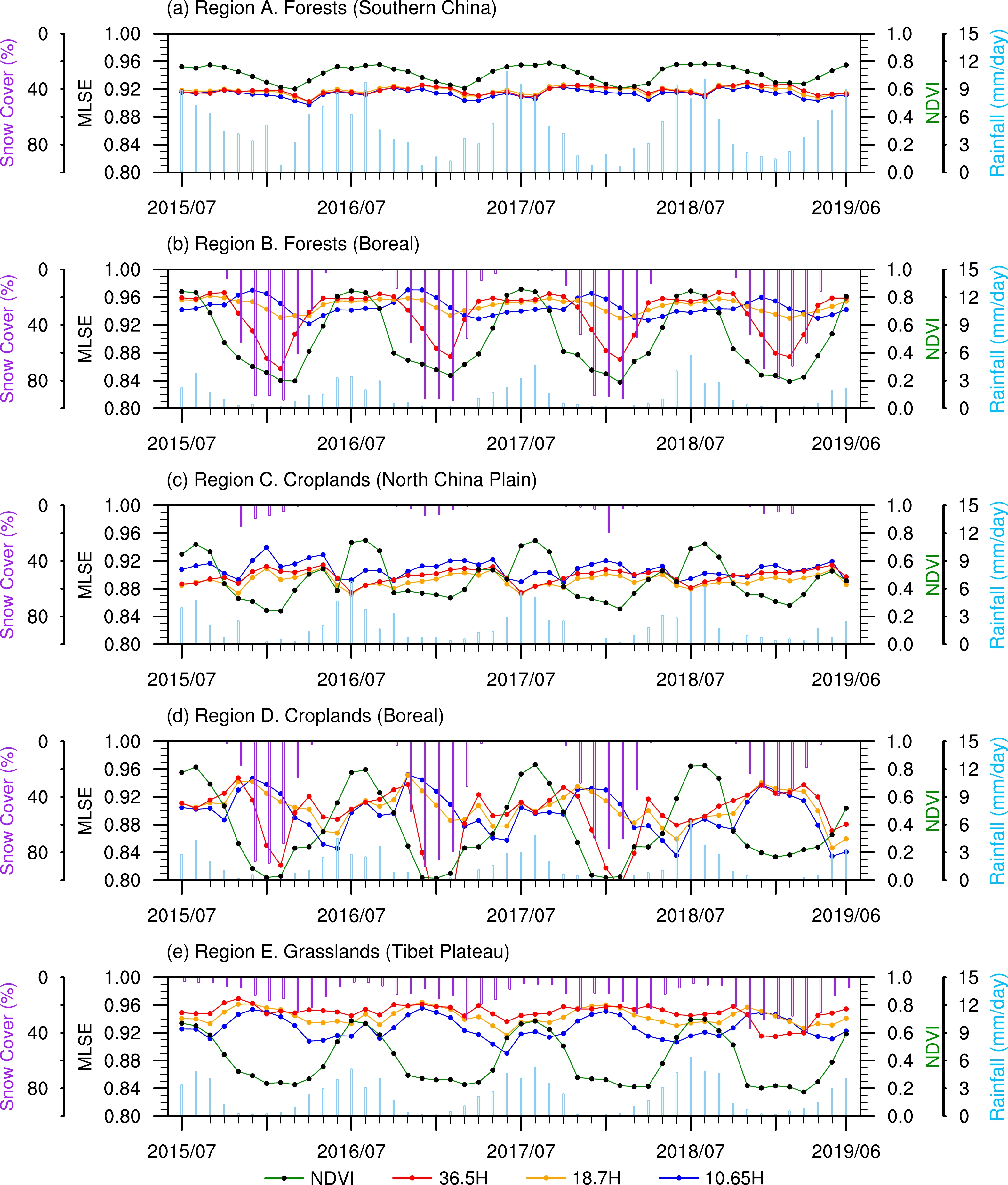
In a given region, the temporal variation of MLSE can reflect the changes of multiple land surface properties, including soil moisture, vegetation, precipitation, snow cover, etc. In order to study the temporal variations of MLSE in China with different types of land cover, we selected eight regions (Fig. 6, Table 4), including two mixed forests (A, B), two croplands (C, D), two grasslands (E, F), one island with mixed tropical forest, savannas (G), and one desert (H). Time series analyses (Figs. 7 and 8) of MLSE were performed in these regions on monthly basis along with NDVI, GPCP monthly precipitation, and MYD13C2 snow cover.

Figure 6. Selected regions for studying seasonal variations of MLSE in China. Overlapped is the IGBP land cover type in 2010 from MCD12C1 (Sulla-Menashe and Friedl, 2015).
Regions Vegetation zone Longitude (E)/
Latitude (N)Proportions of different land types (%) Barren Forests Crop Grass and
shrubsSavannas Urban and
build-upsWater A Subtropical evergreen broadleaf forest 106°–112°/22°–25° <0.01 33.1 16.9 0.04 49.1 0.61 <0.01 B Evergreen coniferous forest 119°–125°/50°–53° <0.01 93 4.9 1.56 0.45 0.06 <0.01 C Temperate deciduous broadleaf forest 114°–118°/35°–38° 0.02 0.8 97.8 0.23 <0.01 1.14 0.27 D Temperate grassland 123°–128°/47°–49° <0.01 1.0 97.1 1.22 <0.01 0.22 0.38 E Qinghai-Xizang Plateau vegetation 97°–102° /30°–34° <0.01 5.0 <0.01 95 <0.01 <0.01 <0.01 F Temperate grassland 107°–110°/37°–40° <0.01 <0.01 0.89 99.1 <0.01 <0.01 <0.01 G Tropical rain forest 108°–111°/18°–20° 0.08 28.4 38.6 <0.01 32.3 0.17 0.11 H Temperate desert 80°–84°/37°–40° 99.9 <0.01 0.02 0.03 <0.01 <0.01 <0.01 Table 4. Proportions of different land types in the eight selected regions.

Figure 7. (Continued).
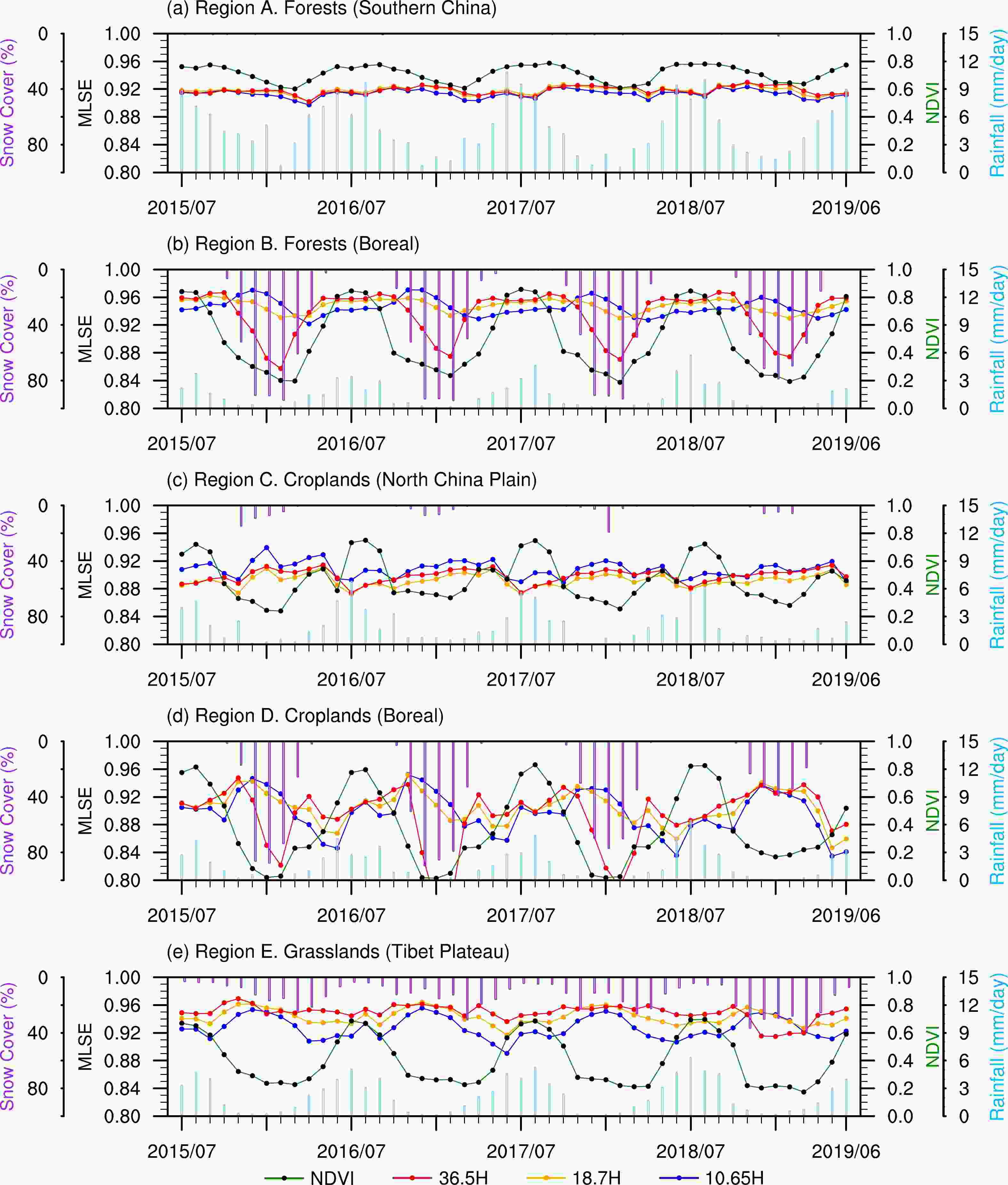
Figure 7. Time series of monthly mean FY-3B MWRI_MLSEs (at 10.65H as blue lines, 18.7H as orange lines, and 36.5H as red lines), GPCP rainfall (sky blue bars), vegetation greenness (NDVI as green lines), and snow cover (purple bars) from July 2015 to June 2019 in selected regions (a) Region A (forest in southern China), (b) Region B (boreal forest), (c) Region C (croplands in the North China Plain), (d) Region D (boreal croplands), (e) Region E (grasslands over the Tibet Plateau), (f) Region F (grasslands over the Loess Plateau), (g) Region G (tropical forest on Hainan Island), and (h) Region H (desert in Xinjiang).
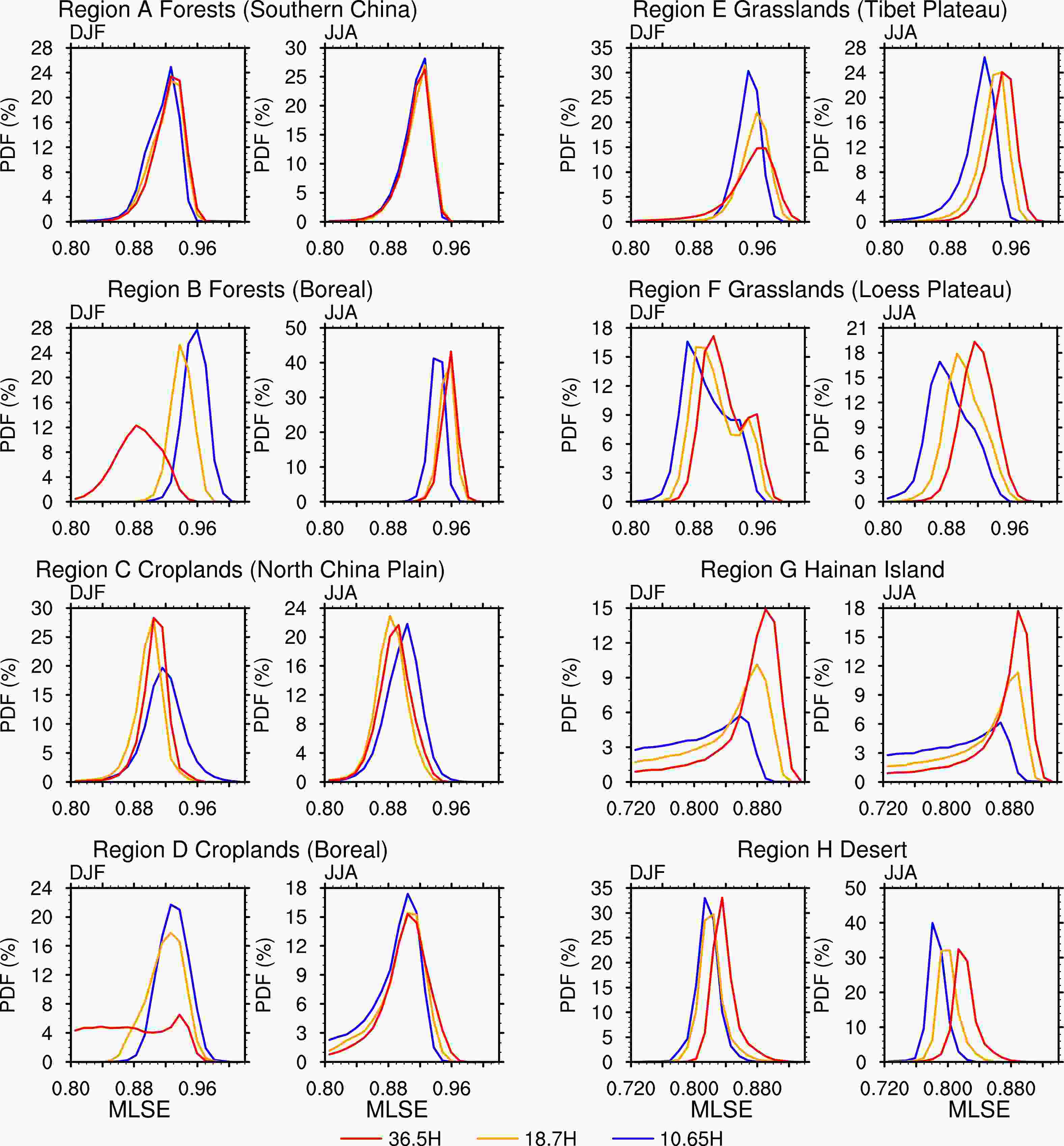
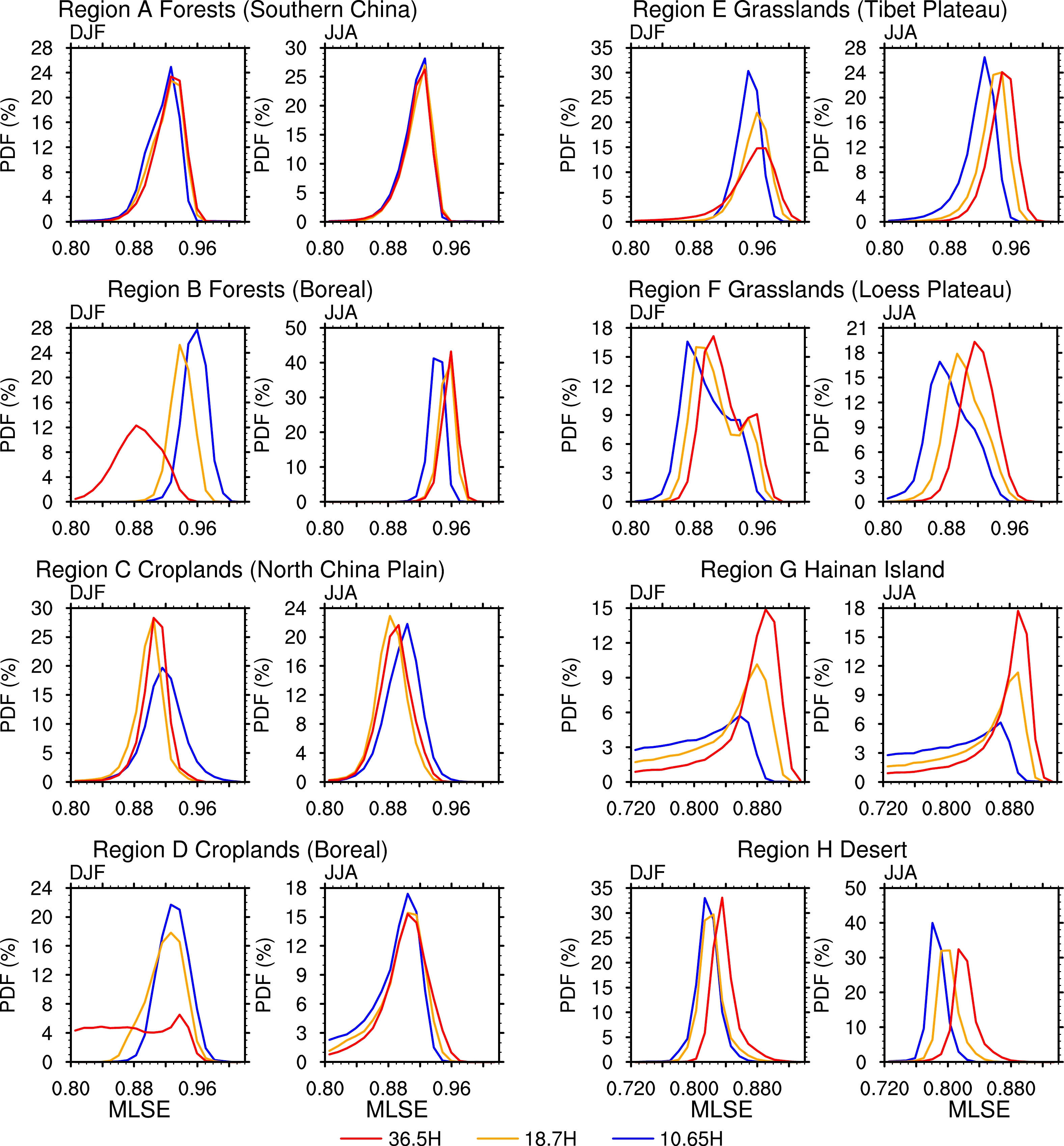
Figure 8. Probability Distribution Function (PDF, %) of MLSEs in winter (DJF) and summer (JJA) at three frequencies (at 10.65H in blue, 18.7H in orange, and 36.5H in red) in the eight selected regions.
In the southern forest Region A (Fig. 7a), the amplitude of the seasonal variation of MLSE is nearly the smallest among all the regions. Generally, the dependence of MLSE on vegetation (indicated by NDVI) and precipitation is not very clear in this region, although we can see the MLSE in winter is a little smaller than that in summer due to the growth of vegetation. In addition, the frequency dependence of MLSE in this region is very weak (Fig. 8a). This is unique because in most other regions, MLSE increases with frequency, except in the situation under snow cover (see further discussions).
In the boreal forest Region B (Fig. 7b), the amplitude of the seasonal variation is nearly the largest among all the regions, and this is obviously driven by snow cover. In winter, when snow cover reaches its maximum in February, the MLSE36.5 (MLSE at 36.5 GHz, hereafter) is the lowest in this region at about 0.84 (compared to 0.92 at Region A). This is because snow particles strongly scatter upwelling microwave radiation, leading to apparent decreases of MLSE. But for lower frequencies such as 10.65 GHz and 18.7 GHz, this effect is much weaker. Still the MLSE10.65 (MLSE at 10.65 GHz, hereafter) and MLSE18.7 (MLSE at 18.7 GHz, hereafter) show decreasing trends from their peak values in November to their minimums in March and April, respectively. It is possible that the melting of snow in these months greatly increases the soil moisture, resulting in minimal MLSEs. It is interesting that the frequency dependence of MLSE changes here between summer and winter (Fig. 8). In summer, MLSE increases with frequency (i.e., MLSE36.5 > MLSE18.7 > MLSE10.65); however, in winter, MLSE decreases with frequency (i.e., MLSE36.5 < MLSE18.7 < MLSE10.65) due to the previously mentioned snow scattering effect. In addition, it is found that there is a weak positive correlation between all MLSE products and NDVI in summer.
In the croplands of the northern China plain, Region C (Fig. 7c), the amplitude of the seasonal variation is also very small. However, significant signals of double-harvest per year in 2016, 2017, and 2018 can be found in NDVI and MLSE. In the months before harvest, NDVI and MLSE reach their peaks and then drop dramatically after harvest. However, the positive response of MLSE to NDVI might be partially compensated by the suppression effect from rainfall, which is heavy in summer (the crop-growing season). There is a weak increasing trend from July to December, most likely because of decreasing rainfall. As shown in Fig. 7, Region C is the only region where the MLSE is higher at a lower frequency than that at a higher frequency in all seasons (i.e., MLSE36.5 < MLSE18.7 < MLSE10.65). We speculate that the grain has a scattering effect, similar to the effect of snow particles as mentioned for Region B, and this effect decreases the upwelling microwave radiation, particularly at high frequencies.
In the boreal cropland Region D, the temporal variation is very similar to that in Region B. Also, we found large-amplitude seasonal variation due to snow. The MLSE36.5 reaches its minimal value of 0.8 or lower in February. And the MLSE10.65 and MLSE10.87 reach their minimums at the end of snow-covering season (March-April-May). The frequency dependence of MLSE reverses in winter compared to that in summer (Fig. 8). There is also a weak correlation between NDVI and MLSE.
In the grasslands of the Tibet Plateau, Region E, we found a medium amplitude of seasonal variation. MLSE is larger in fall and winter than in spring and summer. It seems this is negatively correlated to the rainfall. In summer, the increase of vegetation (NDVI) leads to a small peak of MLSE, indicating MLSE increases with vegetation here. In winter, the snow cover here is significant but is relatively lower (by 20%–40%) than in Regions B and D. Consequently, the snow does not cause remarkable suppression of MLSE36.5. In addition, differences in the snow ice microphysics also make distinct differences in the suppression effects. This is highly related to the grain size, snow water equivalent, snow depth, and frozen status. In this area, MLSE increases with increasing frequency in all seasons (Fig. 8, MLSE36.5 > MLSE18.7 > MLSE10.65).
In another grassland in Loess Plateau, Region F, the seasonal variations of NDVI, snow cover, and rainfall are all weaker than those in Region E (also grasslands). Consequently, the amplitude of MLSE seasonal variation is also weaker.
In the tropical mixed forest over Hainan Island, Region G, the seasonal variation is very weak. MLSE shows weak correlation with NDVI but increases during the dry season and decreases during the rainy season due to changes in soil moisture. Due to the impact of water in inland waterbodies and coasts, the MLSE 10.65 is very low in this region, which is also evidently demonstrated by its PDF (Fig. 8).
In the selected desert Region H, the MLSE values are the smallest among all the selected regions. The seasonal variation is medium and clearly driven by snow cover. However, the effect of snow cover on MLSE here is enhancement instead of suppression, as seen in other regions. It is possibly due to the relative difference of dielectric constants between sand grains and snow particles. There is very weak rainfall in JJA in this region, but it seems this does not cause significant impacts on the soil moisture and has no impacts on MLSE.
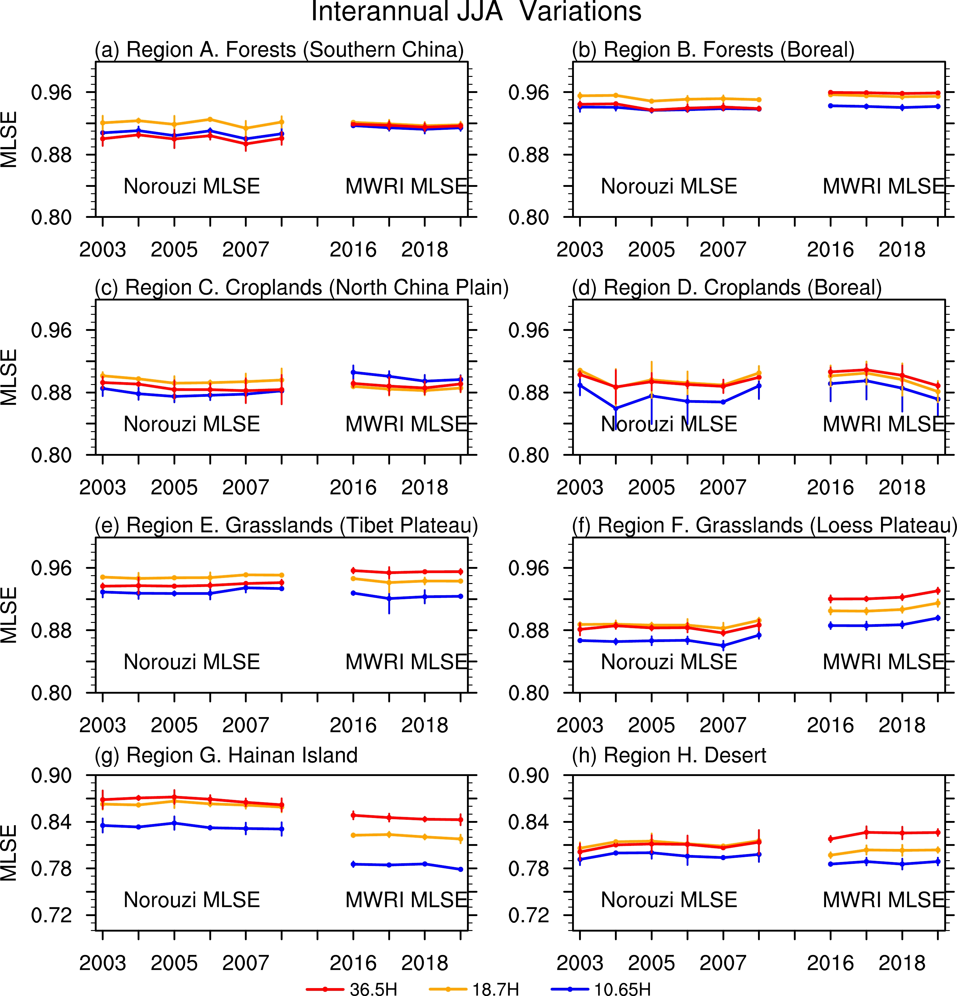
Interannual variations of seasonal mean MLSE from 2003 to 2019 in summer and winter are shown in Figs. 9 and 10 using both AMSR-E (e.g., Norouzi_MLSE) and FY-3B MWRI retrievals. The time series of seasonal mean MLSEs derived from the two sensors show comparable interannual variations in most regions. This again is proof that the measurements and recalibrations of MWRI are reliable and the performance of the MLSE retrieval algorithm works well.
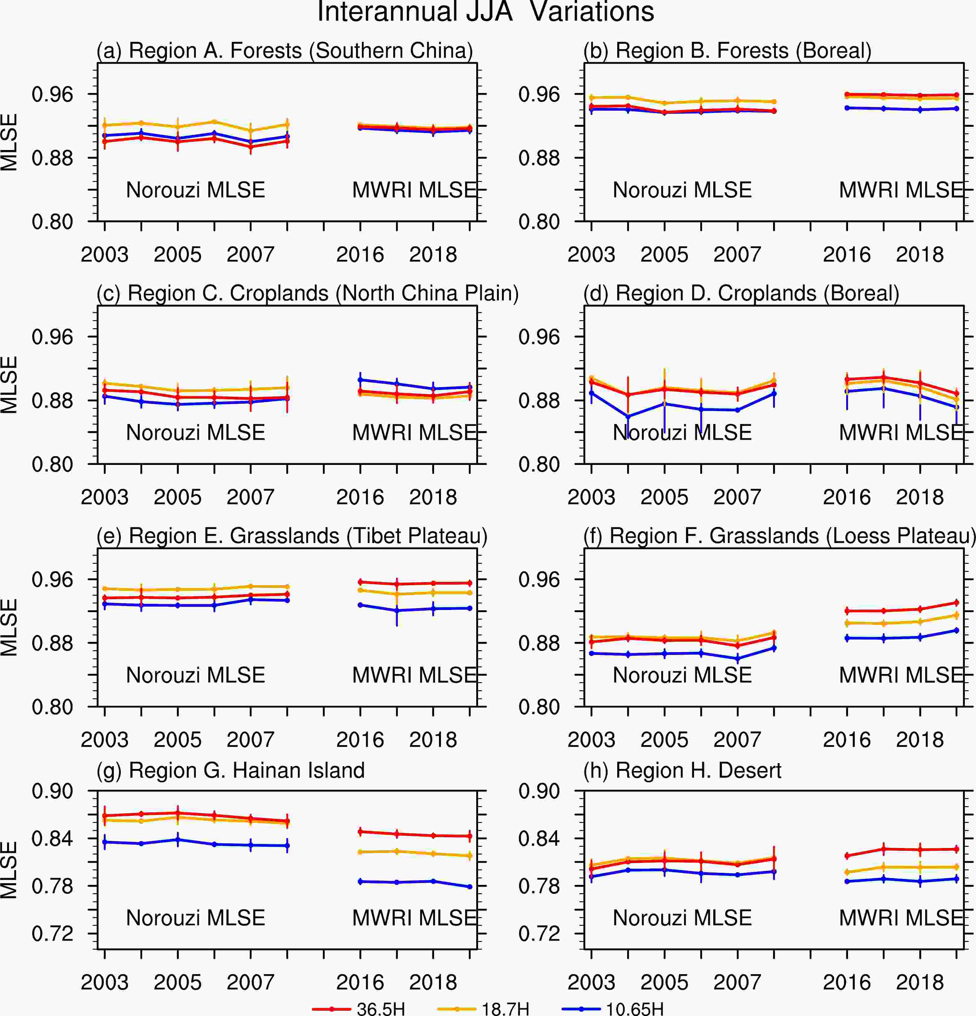
Figure 9. Time series of seasonal mean MLSEs (at 10.65H in blue, 18.7H in orange, and 36.5H in red) in summer (June, July, and August) from 2003 to 2008 derived from AMSR-E (Norouzi_MLSE) and FY-3B MWRI from 2016 to 2019 in the eight selected regions.
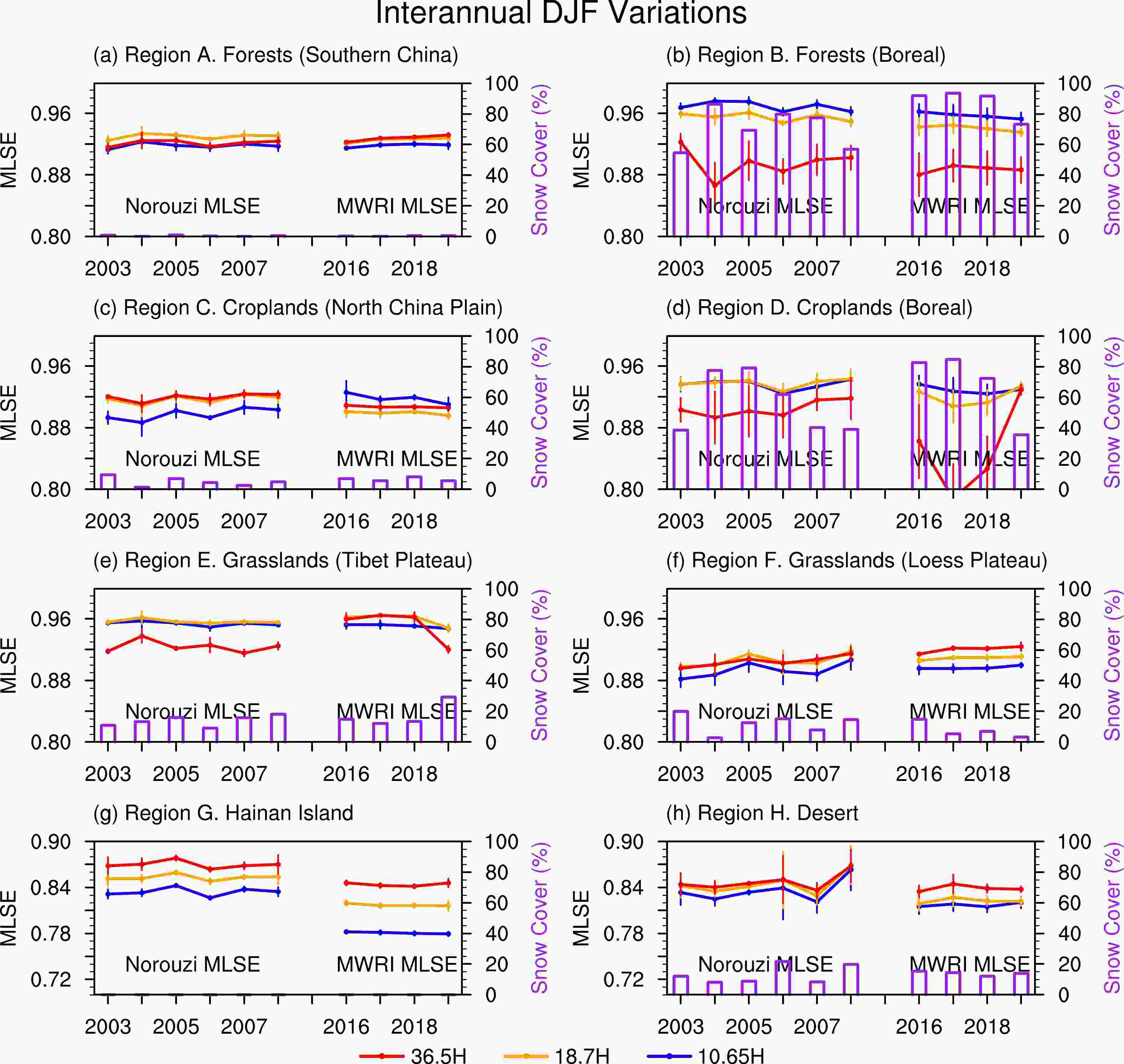
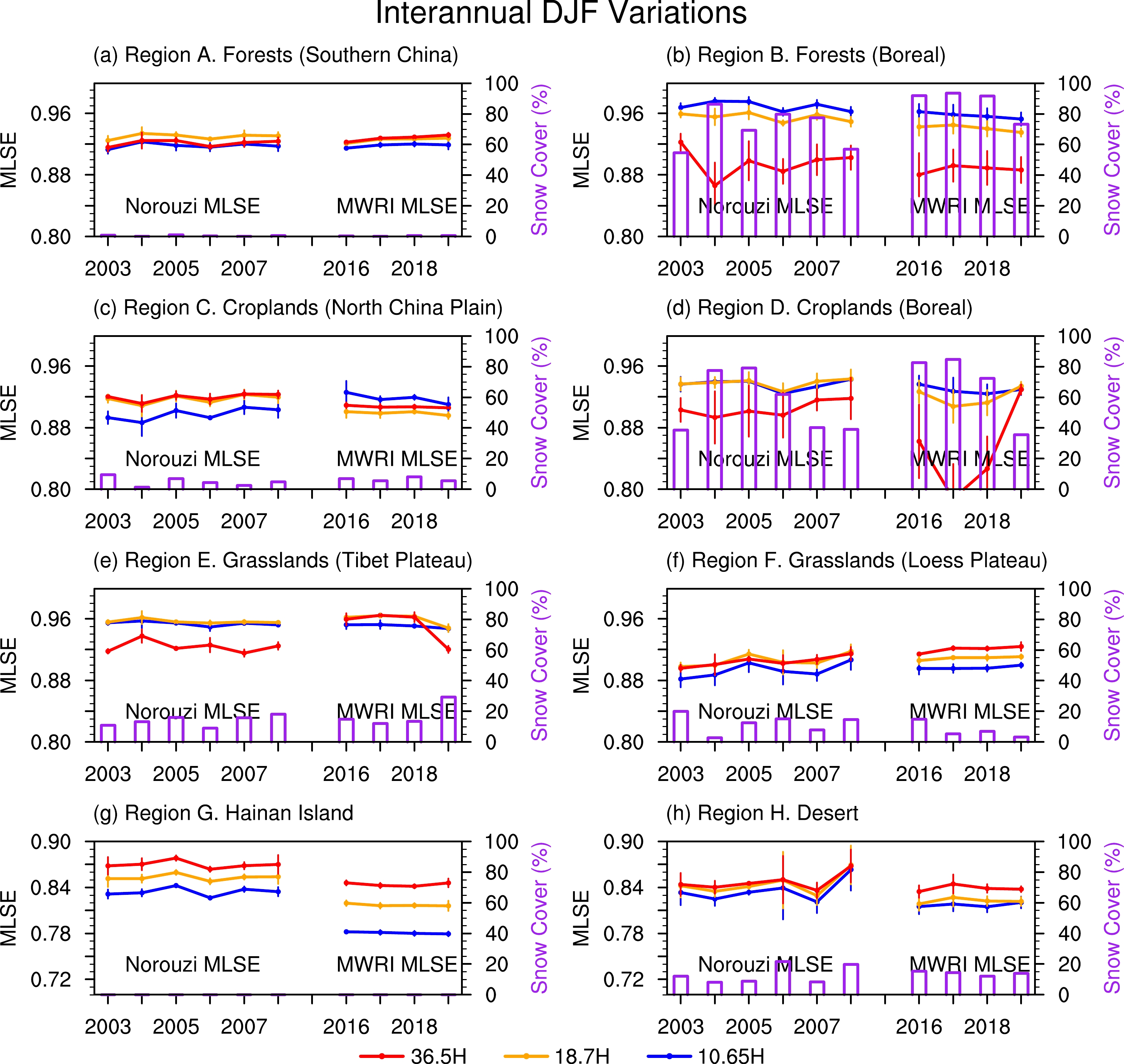
Figure 10. Time series of seasonal mean MLSEs (at 10.65H as blue lines, 18.7H as orange lines, and 36.5H as red lines) in winter (December, January, and February) from 2003 to 2008 derived from AMSR-E (Norouzi_MLSE) and FY-3B MWRI from 2016 to 2019 in the eight selected regions. Overlapped pink vertical bars are associated seasonal mean snow cover (%) derived from MODIS.
It was found that in Hainan Island (Figs. 9g and 10g) there is a significant drop in MLSE, particularly at 10.65 GHz, in FY-3B retrievals in both summer and winter. It indicates that our MLSE retrieval may suffer from severe side lobe effects from open water, particularly in the coastal area. And in Region F, the grasslands in Loess Plateau, the summer MLSE shows a weak increasing trend. It is possible that such changes reflect the real land use and land changes occurring in those regions since the time series in other regions are rather stable. Of course, further in-depth investigations based on long-term data records must be done before we can draw a solid conclusion regarding the long-term trend of MLSE and its causes. In winter, the annual MLSE is heavily affected by the variations of annual snow cover. In the years with greater snow cover, MLSEs at 36.5 GHz from both sensors decrease significantly. This is evident in Region B (the boreal forest), Region D (the boreal croplands), and Region E (the grasslands over the eastern Tibet Plateau).
-
As shown in Fig. 11, the correlations between MLSEs and NDVI vary with different types of land cover and at different frequencies. In forest Region B, MLSEs tend to increase with NDVI at first when NDVI is weaker than about 0.3–0.4, and then MLSEs decrease or tend to be saturated with the further increase of NDVI. This phenomenon is also observed in Region D (the boreal croplands) and in Region E (the grasslands over the Tibet Plateau) and is particularly evident for MLSE36.5. This result is consistent with Li and Min (2013), who pointed out that the response of MLSE to vegetation water content (VWC) could be either positive or negative, depending on the partition between vegetation emission, scattering, and soil emission characteristics. In their study, MLSEs increase when VWC is small and then decrease with VWC when VWC is large. The non-monotonic dependence of MLSE on vegetation is also consistent with the theoretic calculation of Min and Lin (2006b).
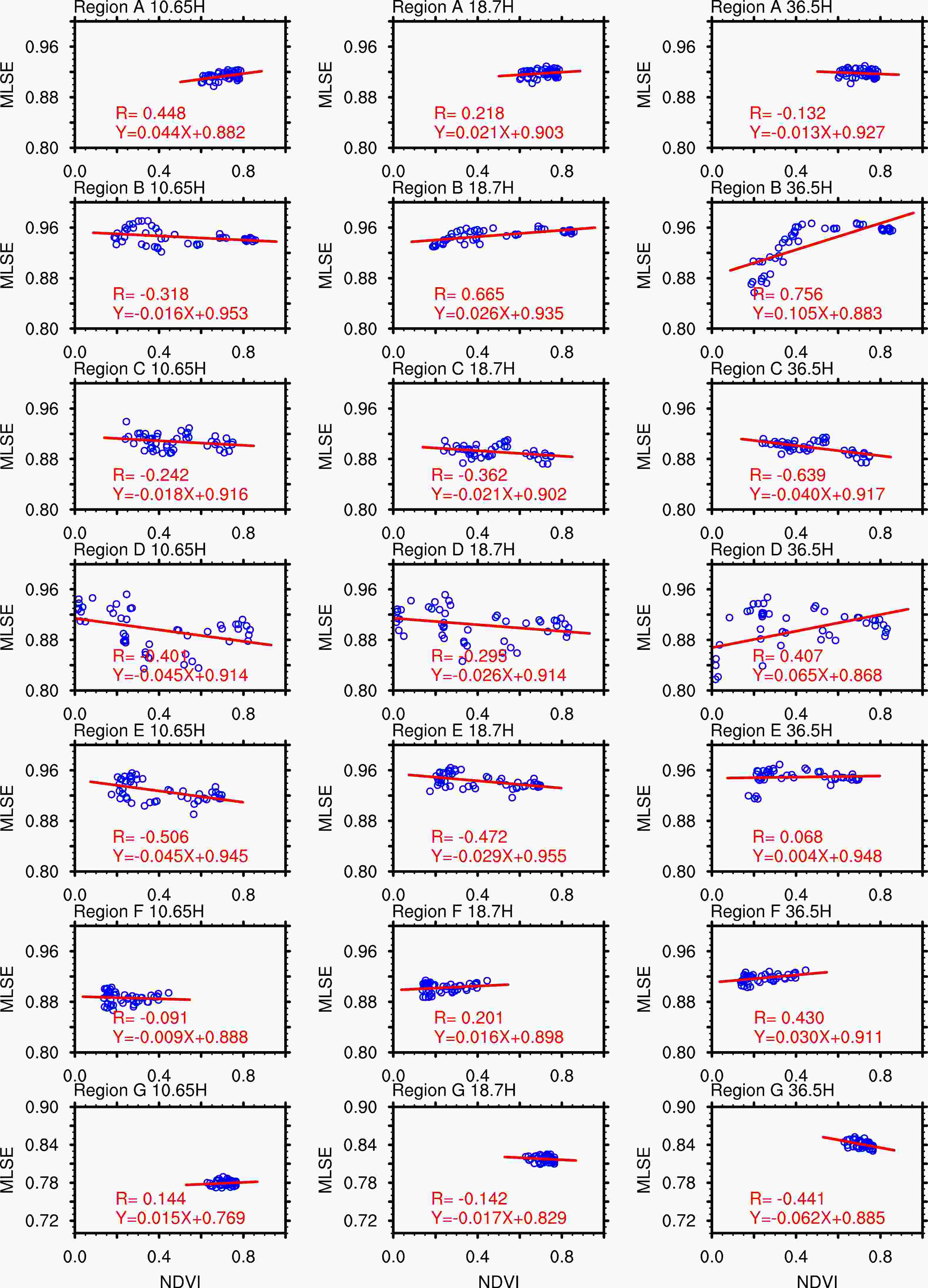
Figure 11. Scatter plots of monthly MLSEs against NDVI in seven selected regions over 2015 to 2019.
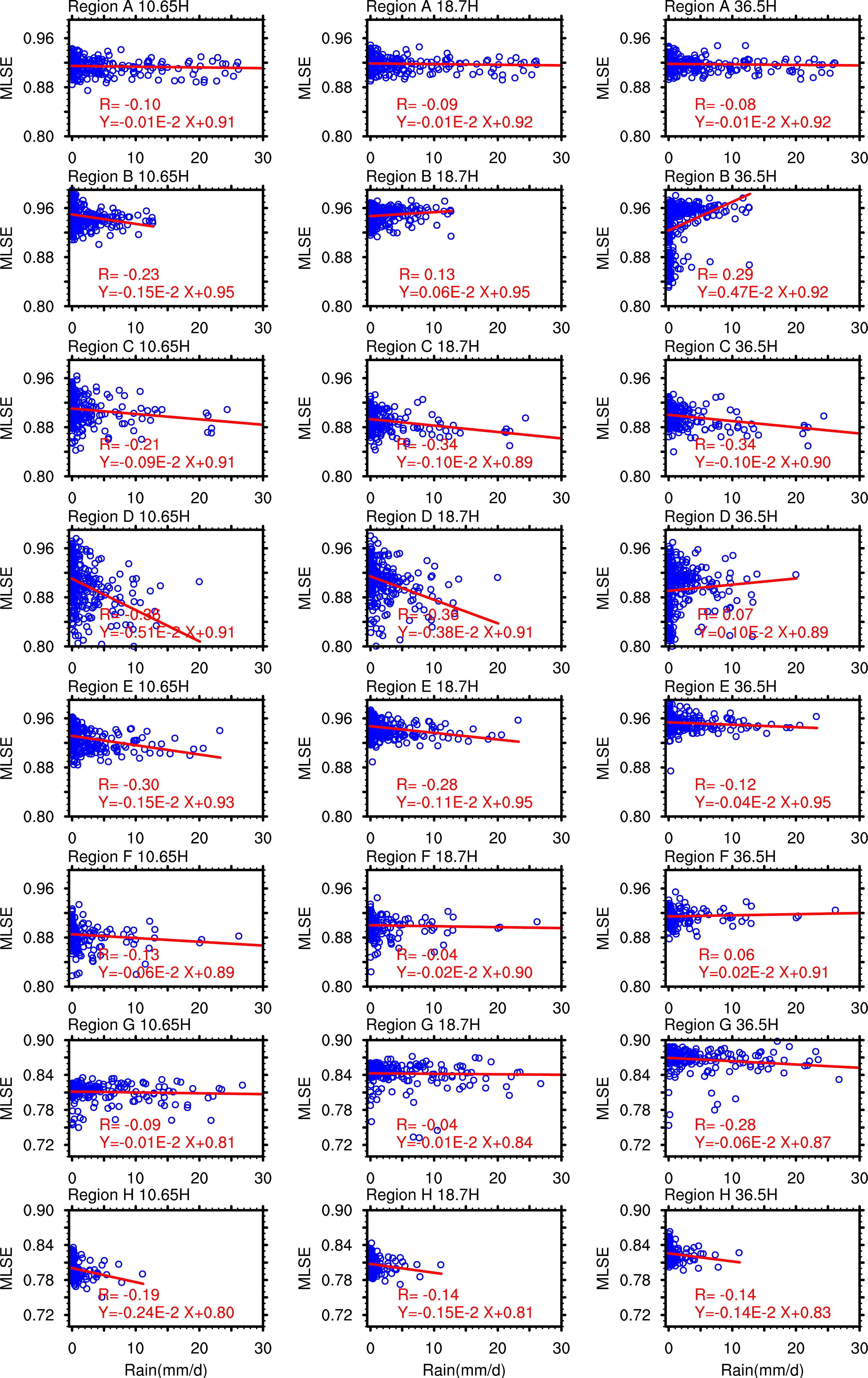
Rainfall has two different impacts on MLSE. First, MLSE is expected to decrease with increasing rainfall due to its enhancement of soil moisture. Second, rainfall favors the growth of vegetation. For instance, vegetation grows with increasing rainfall in spring and generally reaches its mature stage in summer. As suggested in previous studies (Prigent et al., 2005, 2006; Shahroudi and Rossow, 2014; You et al., 2014), surface precipitation can change the soil moisture and associated emissivity within minutes and exert a long-lasting effect after the rain ends. Thus, the analysis of rainfall effects on MLSE should be carried out on the daily scale. As shown in Fig. 12, at the daily scale, there is a negative response of MLSE to increasing rainfall, especially at the lower frequency (10.65 GHz) and in non-forest areas, which indicates soil moisture changes dominate the MLSE variations. However, inherent positive correlations between rainfall and vegetation are still found, which partially compensate the response of MLSE to rainfall (soil moisture), and thus, the observed correlations between MLSE and rainfall are actually weak in most regions, as shown in Fig. 12. In Region B, the MLSE36.5 even increases with increasing rainfall. It appears that at this high frequency, MLSE reacts primarily to the vegetation increase, not to soil moisture variations, which is consistent with Prigent et al. (2006).
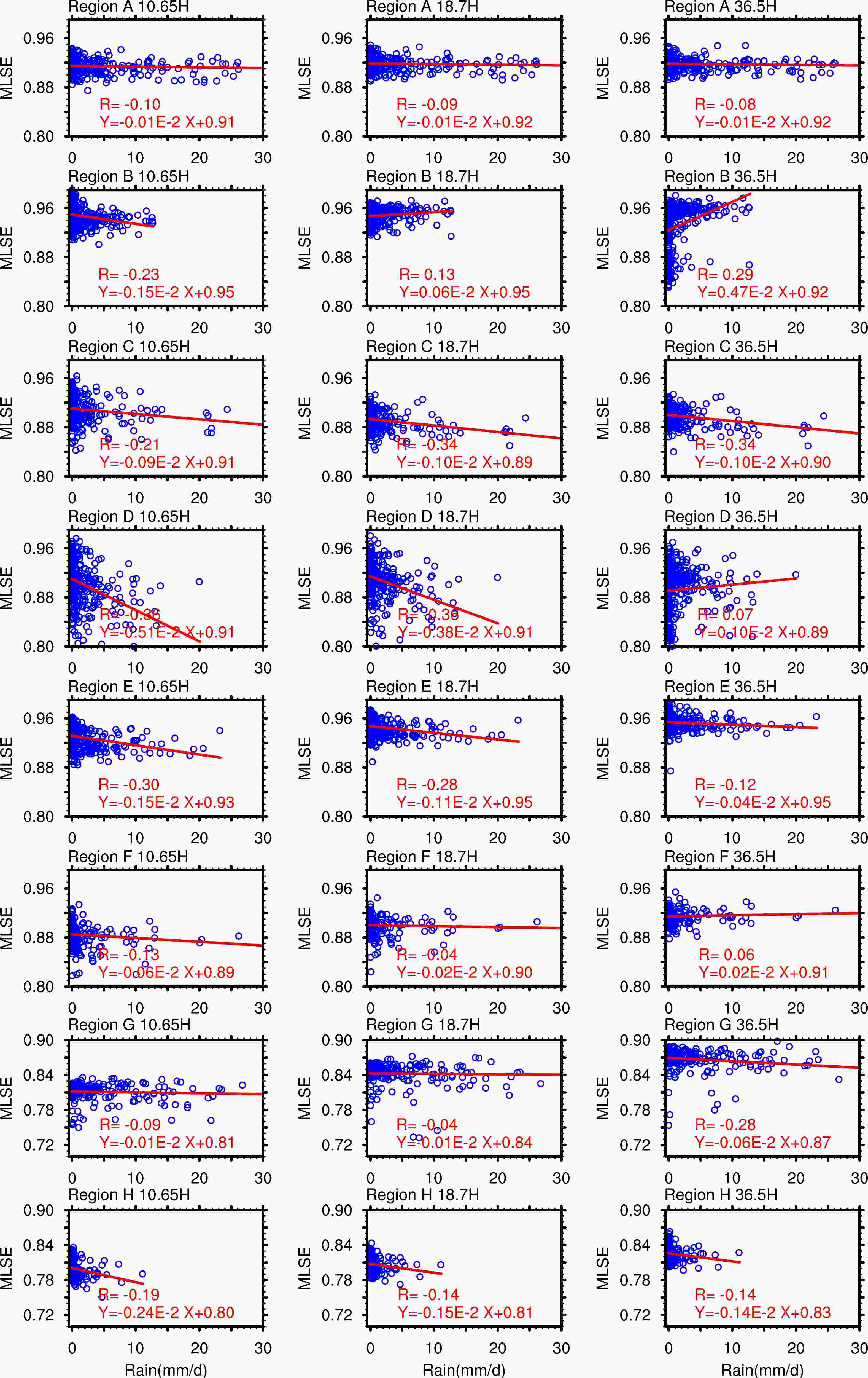
Figure 12. Scatter plots of monthly MLSEs against rainfall in the eight selected regions. Samples are aggregated from daily records of MLSE and GPCP rainfall around the sites in 2016.
In regions with large snow cover of up to 80% (Regions B and D, Fig. 13), the MLSE36.5 significantly decreases with increasing snow cover, and the MLSE10.65 increases with increasing snow cover. The performance of MLSE18.7 is in between. In regions with small-to-medium snow cover of less than 40% (Region C, E, and F, Fig. 13), all MLSEs show weak correlation with snow cover.
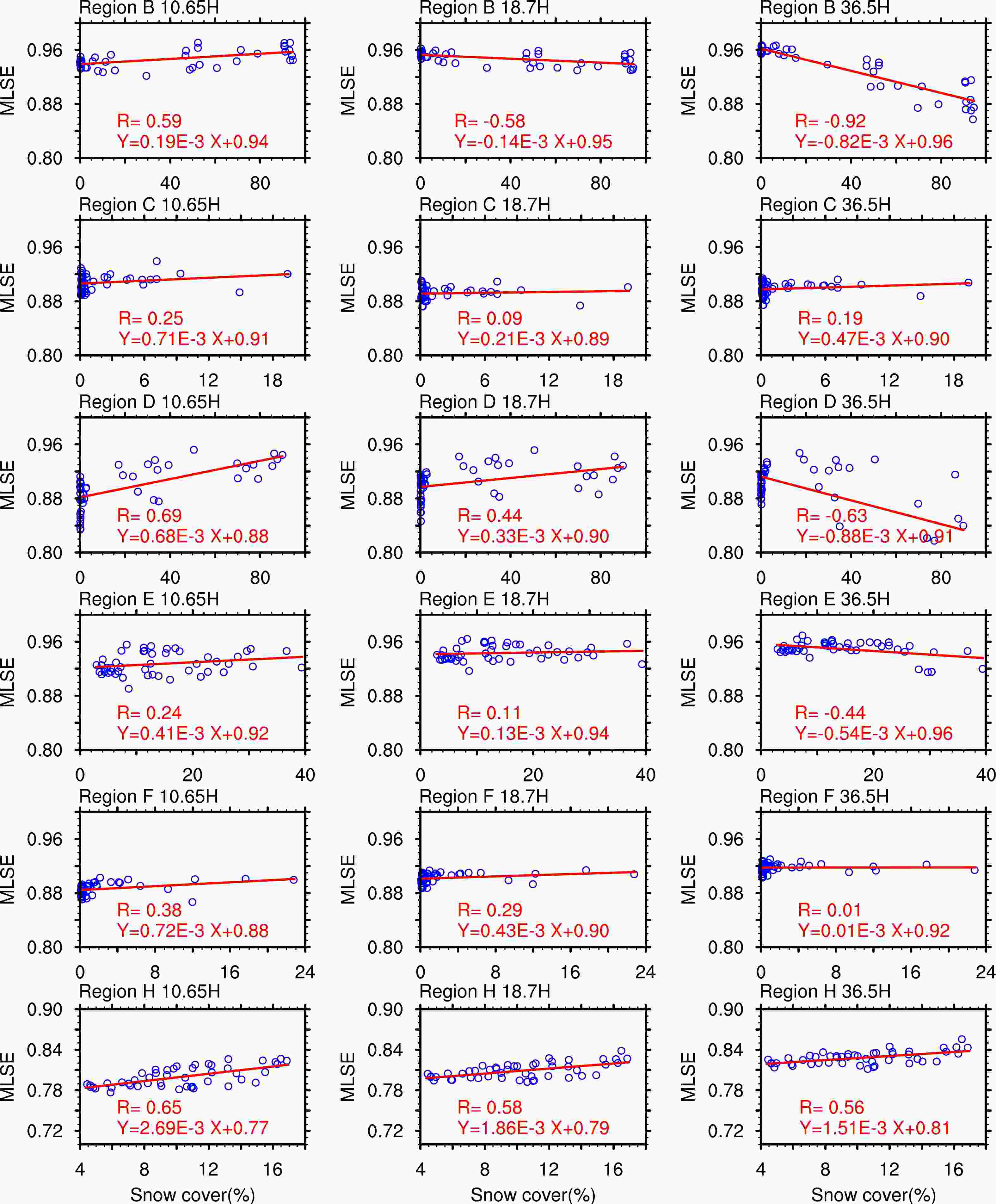
Figure 13. Scatter plots of monthly MLSEs against snow cover in six selected regions over 2015 to 2019.
However, in the desert Region H, all three MLSEs clearly increase with snow cover. This is because the electrical conductivity of dry sand is close to or even lower than that of ice particles (Ulaby et al., 1986). When the sand was covered by snow or wetted by the melting snow, the apparent MLSE increases. However, for other types of land cover, the electrical conductivity of soil under snow is relatively higher. Therefore, the snow generally leads to suppression of MLSE.
-
Numerous studies have been conducted on the accuracy and variability of various MLSE retrieval techniques. Ferraro et al. (2013) studied several MLSE-estimation schemes using observations of different sensors. They found that on the monthly mean time scale, estimates of MLSE varied by as much as 3%, or even greater, for many instantaneous retrievals. For 36.5 GHz, the retrieved MLSEs showed large uncertainties among different techniques, with the discrepancies up to the order of 5%. They also found that discrepancies were smaller at the lower frequencies and greater at the higher frequencies. It should be noted, as one anonymous reviewer pointed out, better agreement at low frequencies might be due to the lower impact of errors in the treatment of the atmosphere and atmospheric RT. In an agricultural region, on a monthly scale, the microwave brightness temperature estimated from surface forward models could be as large as 10 K (at 37 GHz and 85 GHz) higher than those from satellite-based retrievals. Ringerud et al. (2014) also pointed out that differences between satellite retrievals and surface forward model simulations were generally lower than 2%–3% at frequencies lower than 37 GHz. By quantifying the uncertainties in the emissivity retrievals over two types of land surfaces, Tian et al. (2014) reported retrievals from different sensors tended to agree better at lower frequencies than at higher ones, with systematic differences ranging 1%–4% over desert and 1%–7% over rainforest. In a similar study, Norouzi et al. (2015) found that the standard deviation of the products was lowest (less than 0.01) in rain forest regions for all products and highest at northern latitudes, above 0.04 for AMSR-E and SSM/I and around 0.03 for WindSat. As reported in section 3.2, the spatial correlations between our MLSE and Norouzi’s and Moncet’s are 0.87–0.92 for horizontal polarizations and 0.67–0.83 for vertical polarizations in summer. The RMSEs are 0.016–0.022, and the MBs are –0.001–0.024, which are well within ~2.5%. Even though the comparisons are conducted between different observing years, the high consistencies illustrate good performance of the method used in our work. The FY-3B MLSE dataset still needs to be directly evaluated by using ground-based measurements; this is a planned future study in our lab. In the present study, the indirect evaluation by using the AMSR-E dataset was conducted as an alternative.
-
The high temporal availability of Himawari-8/AHI geostationary observations of clouds provides us with the capability of fusing cloud information for MWRI observations. However, the downsides are quite evident. First, the introduction of AHI cloud retrievals prevents the wide application of MWRI retrieval in terms of spatial coverage. That means retrievals can only be conducted within the full disk of Himawari-8, and the westernmost part (longitude < 80oE) of China is not even covered. Second, temporally, there is a small scan time gap between AHI and MWRI since the former has a 10-min sampling interval. The matching of cloud observations with MWRI may be poorly done. Finally, any failure in the Himawari-8 cloud property retrieval will result in sample discard of the corresponding simultaneous MWRI observation. In our quick glance at the retrieval of cloud effective radius over south China, we found a lower than 50% success ratio between 0000–0900 UTC that lasted for nearly 10 days from 20 July 2016. As reported by Shang et al. (2018), comparing to CALIPSO cloud identification over the Tibet Plateau, the false alarm rate and cloud hit rate of AHI cloud cover retrievals are 7.5% and 73.55%, respectively. While for MODIS, the rates are 1.94% and 80.15%, respectively. Letu et al. (2020) compared the retrieved COT and CER for water clouds with MODIS Collection 6 cloud property products and found the correlation coefficients are 0.77 and 0.82, respectively. The COT of ice clouds also shows good consistency, with a correlation coefficient of 0.85. In general, the AHI retrievals perform well in terms of agreement with existing cloud products and can be used as the cloud source in our work, even though at times there are retrieval failures that may result in MWRI sample losses.
-
The derivation of surface emissivity from surface brightness temperature requires an accurate skin temperature (Ts). Skin temperature is highly variable from day to day and has a significant diurnal cycle because of its relation to solar radiation, while emissivity is usually less variable on a day-to-day scale. In addition, clouds can significantly change the incoming solar radiation, temperature, relative humidity, and other environmental conditions which may further influence the physiochemical processes of vegetation (photosynthesis, evapotranspiration, etc.). Consequently, the water content in soil and vegetation, which significantly determines the microwave dielectric constant of land, may change with clouds, too. In addition, the dielectric constant of water may also change with temperature. The potential change of MLSE under cloudy conditions is still an open question.
In the studies of Aires et al. (2001) and Prigent et al. (2003), the emissivity as an intrinsic property was assumed without significant changes between clear and cloudy conditions from which they derived the skin temperature. In our study, this is overturned since we derive emissivity of skin temperature, which is more variable. The quality/accuracy must be carefully assessed before the use of our ERA-Interim Ts. The issue is quite complicated since it is difficult to validate the ERA-Interim Ts with the in situ measurements. Point in situ measurements of Ts at limited sites have disadvantages in representing the effective temperature in a satellite field of view. The temperature of the emitting layer is difficult to determine. Even an accurately validated skin temperature fails to represent the physical thermodynamic temperature of the emitting layer due to the penetrating effects. As a matter of fact, similar work, like Moncet et al. (2011a), attempted to mitigate such an issue by using the Penetration Time Series technique in land surface types like barren soil. Norouzi et al. (2012) used Principal component analysis (PCA) to evaluate the spatial variation of the Tb diurnal cycle to avoid the large amplitudes of the diurnal cycle of skin temperature in the desert.
In our study, we arranged an intercomparison between our ERA-I skin temperature and that from China Meteorological Administration (CMA) first generation 40-yr global atmospheric reanalysis product, CRA-40 (Liu et al., 2017b; Liang et al., 2020), over several months in 2016. By doing this, we expected to gain a roughly comprehensive understanding on the magnitude of the discrepancy and the induced uncertainty to our MLSE retrievals. As shown in Fig. 14, we retrieved separate MLSEs using Ts from ERA-Interim and CRA-40, respectively, as input. The MLSE differences resulting from the Ts differences were studied. Most of the Ts biases were within ±10 K (Fig. 14d). The sensitivity of MLSE to Ts indicates that a 10-K error in Ts may result in MLSE differences of 0.03–0.04 at 10 GHz, 19 GHz, and 37 GHz at horizonal polarizations, which agrees well with previous findings (Yang and Weng, 2011a).
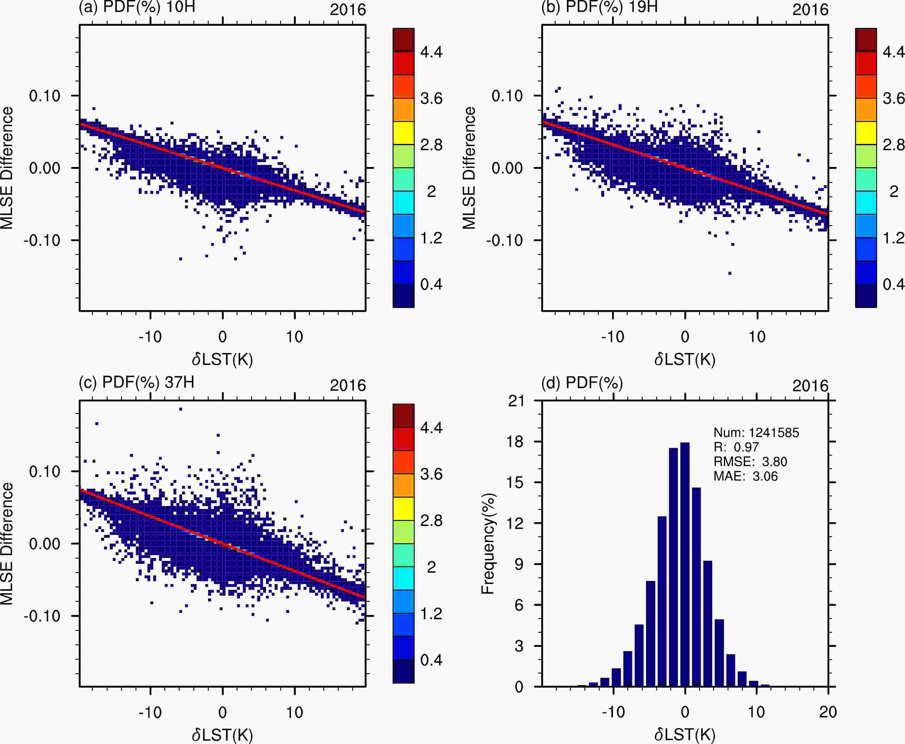
Figure 14. Scatter plots of the differences of MLSEs at 10H (a), 19H (b), and 37H (c) retrieved using two different skin temperatures from ERA-Interim and CRA-40 reanalysis, respectively. δLST = Ts(ERA-Interim) – Ts(CRA-40), and the overlapped color indicates the density of samples. The retrievals are done for four months in 2006 (i.e., January, April, July, and October). (d) The PDF of difference between Ts (ERA-Interim) and Ts (CRA-40).
-
Topographic effects on surface emission and the resulting issues for passive microwave remote sensing have been widely studied. The effects are generally fourfold: the shadowing effect of sky radiation by the surrounding high-elevation terrain (Mätzler and Standley, 2000); the modifications of the atmospheric contributions due to the dependence on the altitude (Kerr et al., 2003); the modifications of the local observing angle caused by the relief angle with respect to the earth coordinate system (Pulvirenti et al., 2008); and the rotation of the linear polarization plane. In an interesting study related to the view angle, the emissivity retrieved from SSM/I was used to derive the emissivity of multiple view angles for SSMT and SSMU (Prigent et al., 2000). Such technology is the same as the rotation of the linear polarization plane, which can be calculated as:
where
${e}'_{p}{{}}$ is the emissivity at p polarization of the rotated plane;$ {\theta }_{\mathrm{l}} $ and α refer to the view angle in the local coordinate system and the rotation angle of the plane with respect to the earth coordinate system, respectively;$ {e}_{p}\left({\theta }_{\mathrm{l}}\right) $ and$ {e}_{q}\left({\theta }_{\mathrm{l}}\right) $ are the original apparent emissivity at dual polarizations. The work of Pulvirenti et al. (2008) studied the relief effects in a simulation of a conically-scanning radiometer similar to AMSR-E. They pointed out that the changes in local observation angle can result in lower apparent emissivity when compared to flat scenes. In addition, they found that the rotation of the panel can increase the H-pol emissivity and decrease the V-pol emissivity. Li et al. (2014) developed a comprehensive radiative transfer model to simulate the topographic effect and tested it by well-controlled field experiment. The model was applied to analyze the difference between AMSR-E observations and modeled results over the Tibet Plateau. It turned out that the difference induced could be up to 18 K over intensely rough terrain.In our study, the topographic effect on the view angle variation is found in the mountainous areas around Hu Huanyong line and the edge of the Tibet Plateau. The potential solution to this issue could be the above introduced methods. But it should be acknowledged that the footprint sizes of sensors like MWRI and AMSR-E are quite big, and thus it will be hard for direct correction in the varied topography in mountainous regions. To solve this problem, using a combined method of forward transfer modeling and the iterative updating of the emissivity guess of subpixels is feasible. This will be addressed in our successive studies.
-
In this study, we developed a retrieval algorithm for microwave land surface emissivity (MLSE) over China based on the measurements of recalibrated microwave brightness temperatures (Tbs) from Fengyun-3B Microwave Radiation Imager (FY-3B MWRI) combined with cloud properties derived from Himawari-8 Advanced Himawari Imager (AHI) observations. A significant feature of this algorithm is the use of cloud retrievals from high temporal resolution geostationary observations. By using a fast and accurate microwave radiative transfer model, the contributions from cloud particles and atmospheric gases to the upwelling Tbs at the top of atmosphere are computed and removed in radiative transfer modeling.
We used this algorithm to build up an MLSE dataset from 7 July 2015 to 30 June 2019 over China and studied its spatial and temporal variations, its consistency with other existing MLSE products, and its dependencies on land cover type, vegetation greenness, rainfall, and snow cover. We mainly focused on MLSEs of horizontal polarizations at 10.7 GHz, 18.7 GHz, and 36.5 GHz.
The spatial distributions in China of MLSE for multiple channels is generally high in the southeast vegetated area and low in the northwest barren, or sparsely vegetated, area. The maximum values of MLSEs (particularly evident for 18.7 GHz and 36.5 GHz) were found in the southwest–northeast oriented belt area of the Qinling-Taihang Mountains and the eastern edge of the Qinghai-Tibet Plateau, which also is the dividing belt between high and low MLSE in China. Very low MLSEs were seen in Xinjiang (e.g., the Taklimakan Desert), western Inner Mongolia, and the Yangtze River delta. MLSEs generally increase with increasing frequency. However, in densely vegetated areas, such as forests in the southeast coastal and northeastern areas of China, MLSE at a lower frequency (e.g., 18.7 GHz) can be larger than that at a higher frequency (e.g., 36.5 GHz).
Despite a significant difference of observing years, the spatial patterns of FY3B-MWRI MLSEs are highly consistent with two selected AMSR-E-based MLSE products. The spatial correlation coefficients between them are 0.87–0.92, and the MBs are only –0.001–0.024. This high consistency indicates that the changes of land surface radiative properties during 2002 to 2019 in China were slow. And it demonstrates the measurements of Tbs by FY-3B MWRI, including its calibration and validation, are reliable, and the retrieval algorithm developed in this study works well.
Temporal variations of monthly mean MLSE in China were studied in eight selected regions, including two mixed forests, two croplands, two grasslands, one island with mixed tropical forest and savannas, and one desert. And the correlations between monthly MLSE to vegetation greenness, rainfall, and snow cover were investigated. Generally, the amplitudes of seasonal variations are small in the southern and tropical forest regions without snow cover in winter. MLSE, to some extent, increases with increasing vegetation greenness, but this effect can be canceled out by the suppression of rainfall. Therefore, MLSE shows weak correlations with vegetation greenness and rainfall. The impact of snow on the seasonal variation of MLSE is evident in the boreal forest and cropland regions. The MLSE36.5 significantly decreases with increasing snow cover and reaches its minimum in the month of the largest snow cover. Meanwhile, the snow scattering effects on MLSE10.65 and MSLE18.7 are much weaker. Instead, they are dominated more by soil moisture and reach their minimums in the spring months (MAM) due to the melting of snow. In addition, it is interesting to find that the MSLEs in the desert increase with increasing snow cover.
The frequency dependence of MLSE in China is complicated. Generally, as reported in the literature, MLSE increases with increasing frequency (i.e., MLSE36.5 > MLSE18.7 > MLSE10.65) in most regions and at most times. However, due to the snow scattering effect, MLSE36.5 in the boreal forest and boreal croplands becomes smaller than MLSEs at lower frequencies in winter. In addition, in the croplands in northern China, MLSE10.65 is greater than MLSE36.5 in all seasons.
The comparison of our MLSE retrieval with the different MLSE retrievals of previous studies indicates that our retrieval is reasonable, given that the error with respect to both Moncet and Norouzi MLSEs is well within 2.5%, which is accepted as relatively small in the literature. We also discussed the downsides of using Himawari-8 AHI cloud retrievals as inputs: extra limitations to the spatial coverage; temporal mismatch; and sample loss to MWRI MLSE retrieval. Then, the quality of the cloud retrievals was discussed.
We further discussed the uncertainties introduced by the skin temperature from ERA-Interim. We arranged another retrieval test using CRA-40 skin temperature to compare with ERA-Interim. It turned out that the Ts difference was within ±10 K, which could result in MLSE differences of 0.03–0.04 for 10H, 19H, and 37H. The view angle issues induced by varied topography were also discussed. Though not resolved in the present work, a feasible method was discussed and is expected to be applied to the problem in future studies.
Based on our knowledge, this is the first all-weather MLSE product based on FY-3B MWRI measurements over the whole of China. The spatial and temporal characteristics of this product confirm the known land surface microwave radiative properties reported in the literature. More importantly, its correlation with vegetation, rainfall, and snow cover widens our understanding of the response of land surface to those environmental controlling factors. There is great potential for using this product in developing physical-based retrieval of atmospheric parameters over land, remote sensing of land surface properties, and the assessment of fire and drought risk.
Acknowledgements. This work was supported by the National Natural Science Foundation of China (Grant Nos. 41830104, 41661144007, 41675022, and 41375148), National Key Research and Development Program of China (Grant No. 2017YFC1501402), and the Jiangsu Provincial 2011 Program (Collaborative Innovation Center of Climate Change).
| Frequencies (GHz) | ||||||
| 6.925 | 10.65 | 18.7 | 23.8 | 36.5 | 89.0 | |
| MWRI sensitivity (K) | − | 0.5 | 0.5 | 0.5 | 0.5 | 0.8 |
| AMSR-E sensitivity (K) | 0.3 | 0.6 | 0.6 | 0.6 | 0.6 | 1.1 |


 AAS Website
 AAS WeChat