


 DownLoad:


-
Heavy rainfall is one of the most serious meteorological disasters that occur in China and is the main contributor to flash flooding and secondary geological hazards, such as landslide and debris flow, causing great economic losses and casualties every year. Studies have shown that heavy rainfall events occur in North China less frequently than in South China, but those in North China are often accompanied by strong convection with large precipitation totals over short time periods (Zhang and Zhai, 2011; Luo et al., 2016; Zhao and Sun, 2019). Meanwhile, local heavy rainfall centers with a small scale and strong intensity are easily formed in North China due to the unique topography and complex underlying surface (Sun et al., 2006; Sun and Yang, 2008; Li et al., 2015). For example, the extremely heavy rainfall event that occurred in Henan province in August 1975, with maximum accumulative precipitation of 1631 mm, caused the collapse of reservoirs and dams, resulting in 26 000 deaths and direct economic losses of nearly 10 billion Yuan (Ding, 2015). The record-breaking heavy rainfall event that occurred in Beijing on 21 July 2012, with rainfall amounts exceeding 460 mm in 18 h, caused severe urban waterlogging and landslides in mountainous areas, resulting in 79 deaths and direct economic losses of more than 20 billion Yuan (Zhang et al., 2013). These are typical cases of extremely heavy rainfall in North China.
At present, accurate prediction of heavy rainfall events is difficult and challenging for short-range weather forecasting (Sukovich et al., 2014). In fact, the formation of precipitation can be generally divided into two stages: the first stage is the transport and convergence of water vapor, and the condensation or freezing of water vapor to produce clouds; the second stage is the formation of precipitation through cloud microphysical processes (Cui, 2009). Braham (1952) first defined precipitation efficiency (PE) as the ratio of surface rain rate to the inflow of water vapor into the storm through the cloud base. Lipps and Hemler (1986) defined PE as the ratio of total precipitation to total condensation. Li et al. (2002) proposed the concepts of large-scale precipitation efficiency (LSPE) and cloud-microphysical precipitation efficiency (CMPE), which are defined as the ratio of surface rain rate to the sum of surface evaporation and moisture convergence, and the ratio of surface rain rate to the sum of condensation and deposition rates of supersaturated vapor, respectively.
PE is an important physical parameter to connect surface precipitation, cloud microphysical processes, and water vapor convergence. To date, there have been many reports on the PE of different types of precipitation systems in different climatological regions (Market et al., 2003; Chang et al., 2015). For example, Zhou (2013) studied the effects of vertical wind shear, radiation, and ice microphysical processes on the PE of a torrential rainfall event in East China. Chang et al. (2015) compared the PE of two distinct precipitation systems in Taiwan and investigated the dependence of PE on the environmental and microphysical factors. Mao et al. (2018) compared the LSPE and CMPE between cold front precipitation and warm sector precipitation in the Beijing “7.21” rainstorm. Brauer et al. (2020) quantitatively studied the change in PE during the landfall of a hurricane based on dual polarization radar observation. Overall, most studies of PE have focused on precipitation systems in the tropics and higher latitudes during the warm season (Li et al., 2002; Sui et al., 2005; Gao and Li, 2011; Xu et al., 2017; Liu and Cui, 2018). The PE of extreme precipitation in North China has rarely been studied.
During the period of 17−22 July 2021, an extremely heavy rainfall event occurred in Henan province in North China, hereafter referred to as the “21.7” Henan rainstorm. The hourly rainfall rate at Zhengzhou station was up to 201.9 mm h−1 from 0800 UTC to 0900 UTC 20 July, which broke the record for the Chinese mainland. In this study, the “21.7” Henan rainstorm was numerically simulated using the Weather Research and Forecasting (WRF) model, and the LSPE and CMPE of the rainstorm were analyzed based on the simulation results. Through analysis of the detailed model simulations, we aim to answer the following questions: What are the key physical factors affecting LSPE and CMPE? And what are the possible mechanisms that lead to high LSPE and CMPE in Zhengzhou?
The rest of the paper is organized as follows: section 2 introduces the data and methodology. Section 3 is an overview of the “21.7” Henan rainstorm and the synoptic conditions. Verification of model results against observations are discussed in section 4. Section 5 presents the analysis of precipitation efficiency and the possible mechanisms of the heavy rainfall. A summary and further discussion is given in section 6.
-
We used the ERA5 reanalysis data provided by the European Centre for Medium-Range Weather Forecasts (ECMWF) (Hersbach et al., 2020). ERA5 is the fifth generation ECMWF reanalysis for global climate and weather and has a horizontal resolution of 0.25° × 0.25° and a time interval of 1 h. Surface rain gauge observations were provided by the National Meteorological Information Center of the China Meteorological Administration. We also used the operational S-band dual polarization radar observation at Zhengzhou station. The radar operates in the volume coverage pattern 21 (VCP-21) scanning mode, consisting of nine elevation angles: 0.5°, 1.5°, 2.4°, 3.4°, 4.3°, 6.0°, 9.9°, 14.6°, and 19.5°. The temporal resolution of radar reflectivity data is 6 min.
-
A three-dimensional and non-hydrostatic WRF model, version 4.2, was used to simulate the “21.7” Henan rainstorm. The domains and configurations of the model are shown in Fig. 3a and Table 1. The ERA5 reanalysis data was used as the initial and boundary conditions, and the model integrates for 48 h starting from 0000 UTC on 19 July 2021. The integration step of the outer domain was 9 s, and the inner domain was 3 s. In order to introduce large-scale fields consistent with the driving fields, the four-dimensional data assimilation (FDDA) functions were activated by performing grid analysis nudging throughout the model integration. In addition, sea surface temperature (SST) data with a resolution of 1° × 1° from the National Centers for Environmental Prediction (NCEP) was used for SST update during the model integration. A modified Morrison two-moment microphysical scheme was used in our study, in which the cloud droplet number concentration was set to 500 cm−3 for polluted continental cases, and the fall speed parameters of graupel were modified based on the sensitivity experiments.
Parameter Description Model WRF V4.2 Horizontal grid spacing Domain 1: 3 km
Domain 2: 1 kmNesting Two−way nesting Grid points Domain 1: 700×700×51
Domain 2: 601×601×51Model top pressure 50 hPa Cloud microphysical scheme Morrison 2−mom Cumulus convective scheme No Planetary boundary layer scheme YSU Land surface scheme Noah land−surface model Longwave radiation scheme RRTMG Shortwave radiation scheme RRTMG Table 1. Design of the numerical simulation experiment.
-
The methods for calculating PE can be divided into two categories: one is LSPE, which reflects the large-scale environment, and the other is CMPE, which reflects the cloud microphysical processes. The calculation of LSPE is based on the surface precipitation equation by Gao et al. (2005) and Cui and Li (2006), while CMPE is calculated based on the budget of cloud hydrometeors during the precipitation process (Li et al., 2002; Sui et al., 2005). The 3D WRF-based LSPE and CMPE are derived by Mao et al. (2018) as follows:
Surface rainfall budget can be expressed as:
$ {Q}_{\mathrm{W}\mathrm{V}\mathrm{T}} $ ,$ {Q}_{\mathrm{W}\mathrm{V}\mathrm{F}} $ ,$ {Q}_{\mathrm{W}\mathrm{V}\mathrm{E}} $ ,$ {Q}_{\mathrm{C}\mathrm{M}} $ , and$ {Q}_{\mathrm{W}\mathrm{V}\mathrm{S}} $ can be calculated by:Then, LSPE and CMPE can be written as:
Here,
$ {P}_{\mathrm{s}} $ , the surface rain rate, is equal to the sum of water vapor processes, including local atmospheric drying/moistening ($ {Q}_{\mathrm{W}\mathrm{V}\mathrm{T}} $ ), water vapor flux convergence/divergence ($ {Q}_{\mathrm{W}\mathrm{V}\mathrm{F}} $ ), surface evaporation ($ {Q}_{\mathrm{W}\mathrm{V}\mathrm{E}} $ ), and hydrometeor loss/convergence or hydrometeor gain/divergence ($ {Q}_{\mathrm{C}\mathrm{M}} $ ).$ {Q}_{\mathrm{W}\mathrm{V}\mathrm{S}} $ is the net amount of water vapor consumed by microphysical processes.$ H $ is the Heaviside function, where$ H\left(F\right)=1 $ when$ F > 0 $ , and$ H\left(F\right)=0 $ when$F \leqslant 0$ . For example, H(QWVT ) = 1 when QWVT > 0, and H(QWVT ) = 0 when QWVT ≤ 0. H(QWVF), H(QWVS) and H(QCM) are interpreted in the same way, in order to ensure that the calculated LSPE and CMPE range from 0 to 100%.$\left[\left( \right)\right]={\int }_{{z}_{{\rm{b}}}}^{{z}_{{\rm{t}}}}\rho \left( \right){\rm{d}}z$ denotes the mass vertical integration, where$ {z}_{\mathrm{t}} $ and$ {z}_{\mathrm{b}} $ are the top and bottom height of the model atmosphere, respectively.${q}_{\mathrm{v}},\;{q}_{\mathrm{c}},\;{q}_{\mathrm{r}},\;{q}_{\mathrm{i}},\;{q}_{\mathrm{s}},\;\mathrm{ }\;\mathrm{a}\mathrm{n}\mathrm{d}\;{q}_{\mathrm{g}}$ are the mixing ratios of water vapor, cloud water, rainwater, cloud ice, snow, and graupel.$ u\;\mathrm{a}\mathrm{n}\mathrm{d}\;v $ are the zonal and meridional winds, and$ {E}_{\mathrm{s}} $ is the surface evaporation. The microphysical processes in the Morrison scheme are summarized in Table 2.Notation Description $ \mathrm{E}\mathrm{P}\mathrm{R}\mathrm{D} $ Sublimation of cloud ice $ \mathrm{E}\mathrm{P}\mathrm{R}\mathrm{D}\mathrm{G} $ Sublimation of graupel $ \mathrm{E}\mathrm{P}\mathrm{R}\mathrm{D}\mathrm{S} $ Sublimation of snow $ \mathrm{P}\mathrm{R}\mathrm{D} $ Deposition of cloud ice $ \mathrm{P}\mathrm{R}\mathrm{D}\mathrm{G} $ Deposition of graupel $ \mathrm{P}\mathrm{R}\mathrm{D}\mathrm{S} $ Deposition of snow $ \mathrm{P}\mathrm{R}\mathrm{A}\mathrm{C}\mathrm{G} $ Rain-graupel collection $ \mathrm{P}\mathrm{R}\mathrm{A}\mathrm{C}\mathrm{S} $ Rain-snow collection $ \mathrm{P}\mathrm{S}\mathrm{A}\mathrm{C}\mathrm{R} $ Conversion due to collection of snow by rain $ \mathrm{P}\mathrm{I}\mathrm{A}\mathrm{C}\mathrm{R} $ Change QR, ice-rain collection $ \mathrm{P}\mathrm{R}\mathrm{A}\mathrm{C}\mathrm{I} $ Change QI, ice-rain collection $ \mathrm{P}\mathrm{I}\mathrm{A}\mathrm{C}\mathrm{R}\mathrm{S} $ Change QR, ice-rain collision, added to snow $ \mathrm{P}\mathrm{R}\mathrm{A}\mathrm{C}\mathrm{I}\mathrm{S} $ Change QI, ice rain collision, added to snow $ \mathrm{P}\mathrm{G}\mathrm{S}\mathrm{A}\mathrm{C}\mathrm{W} $ Conversion to graupel due to collection droplet
by snow$ \mathrm{P}\mathrm{G}\mathrm{R}\mathrm{A}\mathrm{C}\mathrm{S} $ Conversion to graupel due to collection rain by snow $ \mathrm{P}\mathrm{S}\mathrm{A}\mathrm{C}\mathrm{W}\mathrm{G} $ Change in Q collection droplets by graupel $ \mathrm{P}\mathrm{S}\mathrm{A}\mathrm{C}\mathrm{W}\mathrm{I} $ Change Q droplet accretion by cloud ice $ \mathrm{P}\mathrm{S}\mathrm{A}\mathrm{C}\mathrm{W}\mathrm{S} $ Change Q droplet accretion by snow $ \mathrm{M}\mathrm{N}\mathrm{U}\mathrm{C}\mathrm{C}\mathrm{R} $ Contact freezing of rain $ \mathrm{E}\mathrm{V}\mathrm{P}\mathrm{M}\mathrm{S} $ Melting and evaporation of snow $ \mathrm{E}\mathrm{V}\mathrm{P}\mathrm{M}\mathrm{G} $ Melting and evaporation of graupel $ \mathrm{P}\mathrm{G}\mathrm{M}\mathrm{L}\mathrm{T} $ Melting of graupel $ \mathrm{P}\mathrm{S}\mathrm{M}\mathrm{L}\mathrm{T} $ Melting of snow $ \mathrm{P}\mathrm{R}\mathrm{A} $ Accretion droplets by rain $ \mathrm{P}\mathrm{R}\mathrm{C} $ Auto-conversion of droplets $ \mathrm{P}\mathrm{R}\mathrm{E} $ Evaporation of rain $ \mathrm{P}\mathrm{C}\mathrm{C}( > 0) $ Condensation of cloud droplets $ \mathrm{P}\mathrm{C}\mathrm{C}( < 0) $ Evaporation of cloud droplets $ \mathrm{N}\mathrm{P}\mathrm{R}\mathrm{C}1 $ Change NR autoconversion droplets $ \mathrm{N}\mathrm{P}\mathrm{R}\mathrm{A}\mathrm{C}\mathrm{S} $ Change N rain-snow collection $ \mathrm{N}\mathrm{N}\mathrm{U}\mathrm{C}\mathrm{C}\mathrm{R} $ Change N due to contact freezing of rain $ \mathrm{N}\mathrm{R}\mathrm{A}\mathrm{G}\mathrm{G} $ Self-collection of rain $ \mathrm{N}\mathrm{I}\mathrm{A}\mathrm{C}\mathrm{R} $ Change N, ice-rain collection $ \mathrm{N}\mathrm{I}\mathrm{A}\mathrm{C}\mathrm{R}\mathrm{S} $ Change N, ice-rain collision, added to snow $ \mathrm{N}\mathrm{P}\mathrm{R}\mathrm{A}\mathrm{C}\mathrm{G} $ Change N collection rain by graupel $ \mathrm{N}\mathrm{G}\mathrm{R}\mathrm{A}\mathrm{C}\mathrm{S} $ Change N conversion to graupel due to collection
rain by snow$ \mathrm{N}\mathrm{S}\mathrm{U}\mathrm{B}\mathrm{R} $ Loss of NR during evaporation $ \mathrm{N}\mathrm{S}\mathrm{M}\mathrm{L}\mathrm{T}\mathrm{R} $ Change N melting snow to rain $ \mathrm{N}\mathrm{G}\mathrm{M}\mathrm{L}\mathrm{T}\mathrm{R} $ Change N melting graupel to rain Table 2. List of microphysical processes in Morrison microphysics scheme.
-
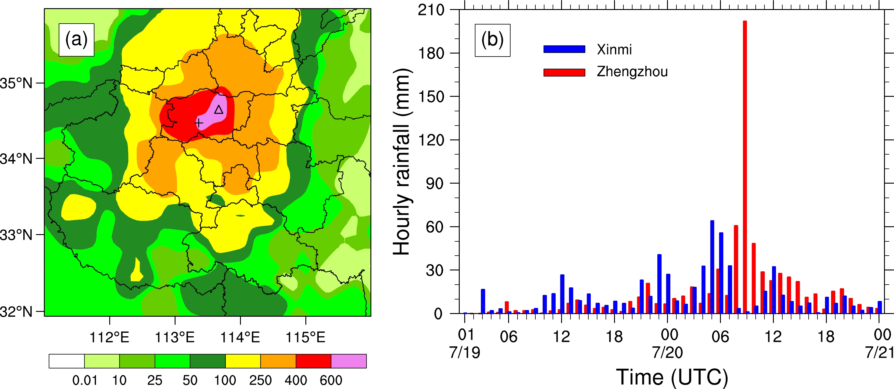
On 17–22 July 2021, an extremely heavy rainfall event occurred in Henan province. Figure 1a shows the accumulative precipitation from 0000 UTC 18 July to 0000 UTC 21 July. It can be seen that a large area of Henan province experienced total accumulated precipitation over 100 mm, and most regions of Zhengzhou experienced heavy rainfall with 72-h cumulative precipitation exceeding 400 mm. The maximum cumulative precipitation was up to 985.2 mm in Xinmi at the Baizhai meteorological station. The hourly rainfall at Zhengzhou station reached 201.9 mm from 0800 UTC to 0900 UTC 20 July, which broke the record of hourly precipitation for the Chinese mainland (Fig. 1b).

Figure 1. (a) The observed accumulative precipitation (units: mm) from 0000 UTC 18 July to 0000 UTC 21 July 2021, “△” and “+” denote the locations of Zhengzhou and Xinmi station, respectively; (b) Time series of hourly rainfall at Zhengzhou and Xinmi station.
The heavy rainstorm brought severe urban waterlogging and landslides in the mountainous areas and caused great damages to Zhengzhou’s road infrastructure, underground railway tunnels, and power grid. It left 292 people dead and 1.88 million people affected, and the direct economic loss was 53.2 billion Yuan (Su et al., 2021).
-
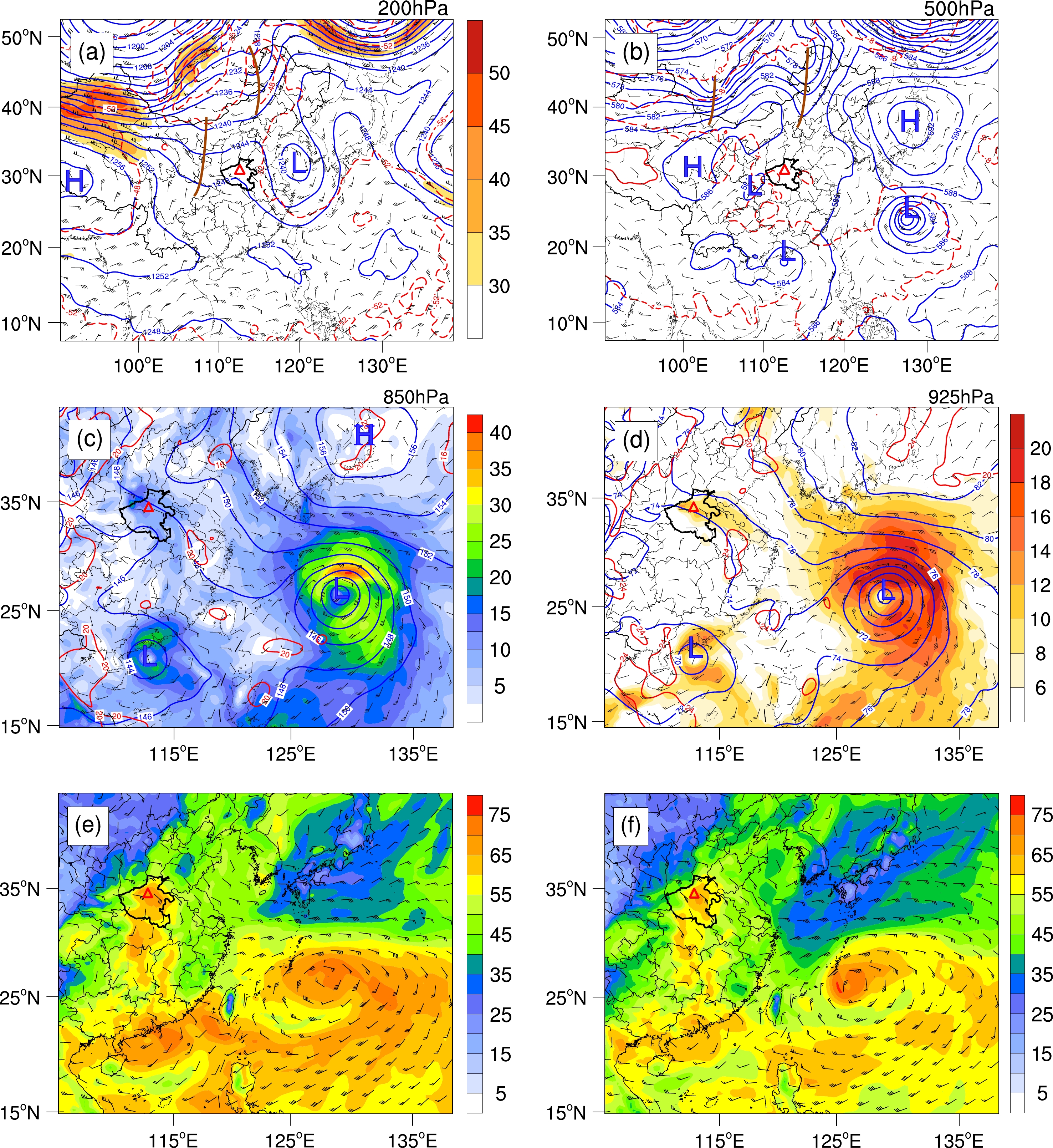
Figure 2 shows the large-scale circulations at 0000 UTC on 19 July 2021 derived from the ERA5 reanalysis data. At 200 hPa (Fig. 2a), the large-scale circulation was characterized by the existence of a South Asian high over the Qinghai–Tibet Plateau, a low pressure center over the East China Sea, and a trough over northern and central China. Henan was under the influence of the high pressure in front of the trough. At 500 hPa (Fig. 2b), the subtropical high jumped northward to 45ºN with the contour of 588 dagpm extending to the east of Jilin province. The continental high dominated over northwest China, and Typhoon In-Fa (2021) and Typhoon Cempaka (2021) were over the East China Sea and the South China Sea, respectively. Henan was on the east side of a low vortex (Huang-huai cyclone). At 850 hPa (Fig. 2c), Henan was located in the typhoon inverted trough on the west side of the subtropical high and experienced prevailing southeasterly air flow owing to the cyclonic circulation of Typhoon In-Fa (2021) and anticyclonic flow of the subtropical high. Abundant water vapor was transported from the ocean to Henan province. At 925 hPa (Fig. 2d), there was a southeast jet extending from the southeast coastal area of China to Henan, which provided necessary dynamic and moisture conditions for the rainstorm.
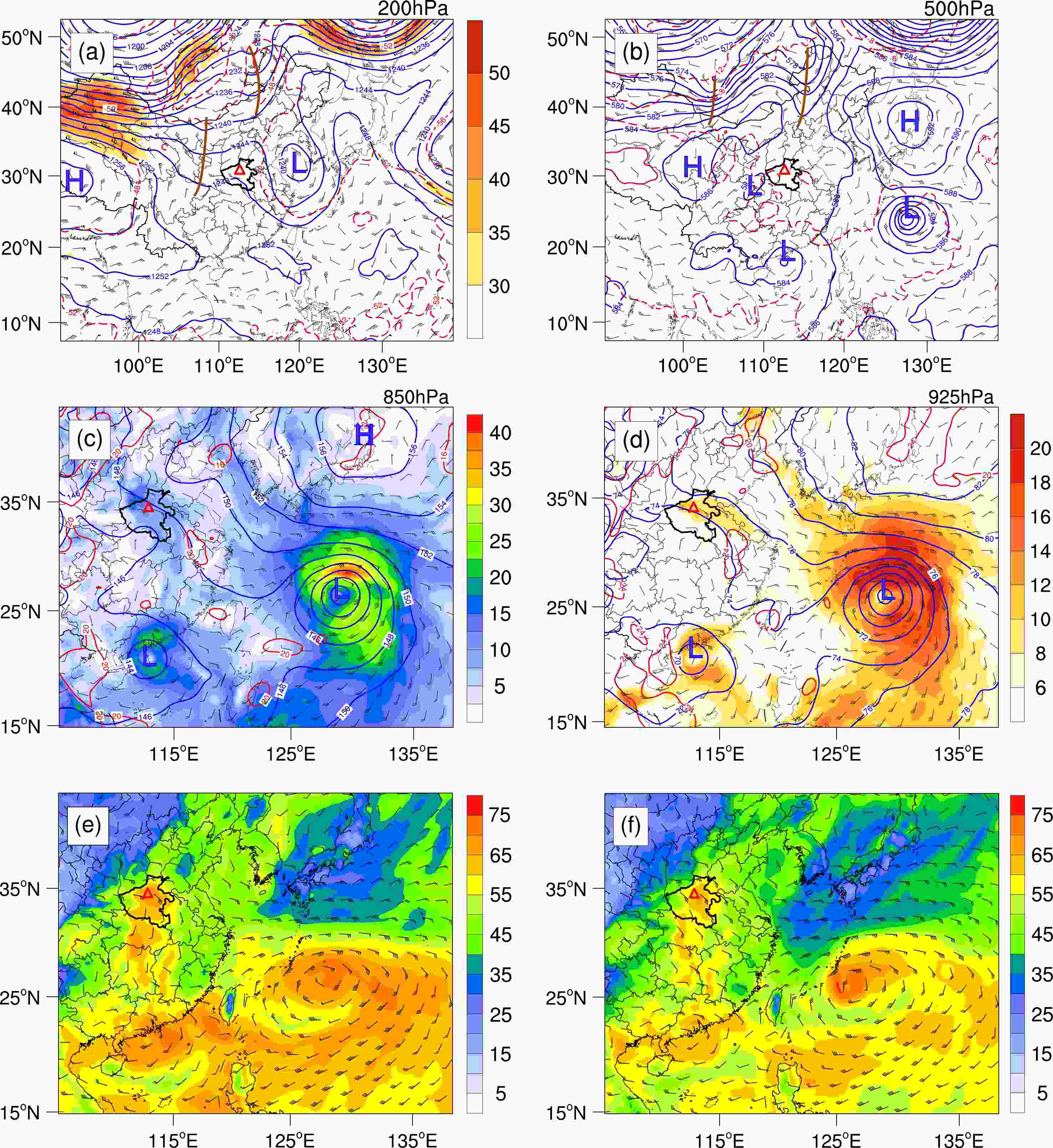
Figure 2. Large-scale circulations at 0000 UTC on 19 July 2021. (a) Geopotential height (blue contours, units: dagpm), wind field (barbs, full barb denotes 4 m s−1), temperature (red contours, units: °C), upper-level jet (shading, units: m s−1) at 200 hPa; (b) Geopotential height, wind field and temperature at 500 hPa; (c) Geopotential height, wind field, temperature and water vapor flux (shading, units: g s−1 hPa−1 cm−1) at 850 hPa; (d) Geopotential height, wind field, temperature and low-level jet (shading, units: m s−1) at 925 hPa; (e–f) Atmospheric precipitable water (shading, units: mm) and wind vector at 850 hPa (barbs). The boundary of Henan province is shown in bold. The red triangle indicates the location of Zhengzhou, and “H” and “L” represent high and low pressure.
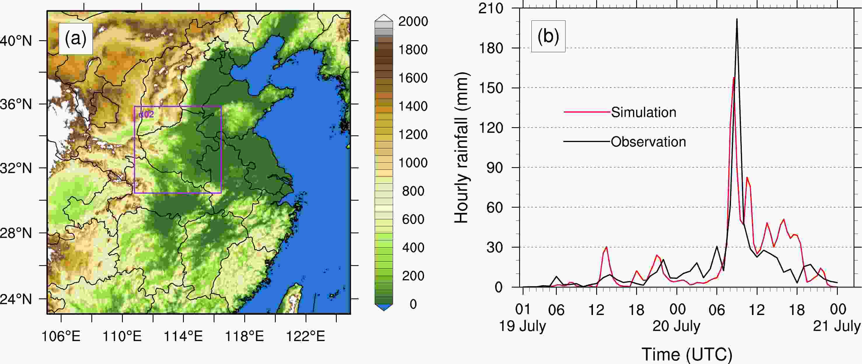
Figure 3. (a) Topography of the simulation domains (units: m); (b) Time series of hourly rainfall rate at the station/location where the maximum hourly rainfall occurred.
In order to further understand the moisture conditions of the rainstorm, we show the atmospheric precipitable water (PW) in Figs. 2e–f. It can be seen that a high PW region extended from the center of Typhoon Cempaka (2021) to the northern part of Henan, passing through Guangdong, Hunan, and Hubei provinces. The southerly air flow crossed the high PW region and transported water vapor to Henan province. Another high PW region with lower intensity was located from the East China Sea to Henan, passing through Zhejiang and Anhui provinces. Water vapor was transported to Henan by the southeasterly flow between Typhoon In-Fa (2021) and the subtropical high. The two moisture transport channels converged in the northern part of Henan, providing sufficient water vapor for the rainstorm (Ran et al., 2021).
-
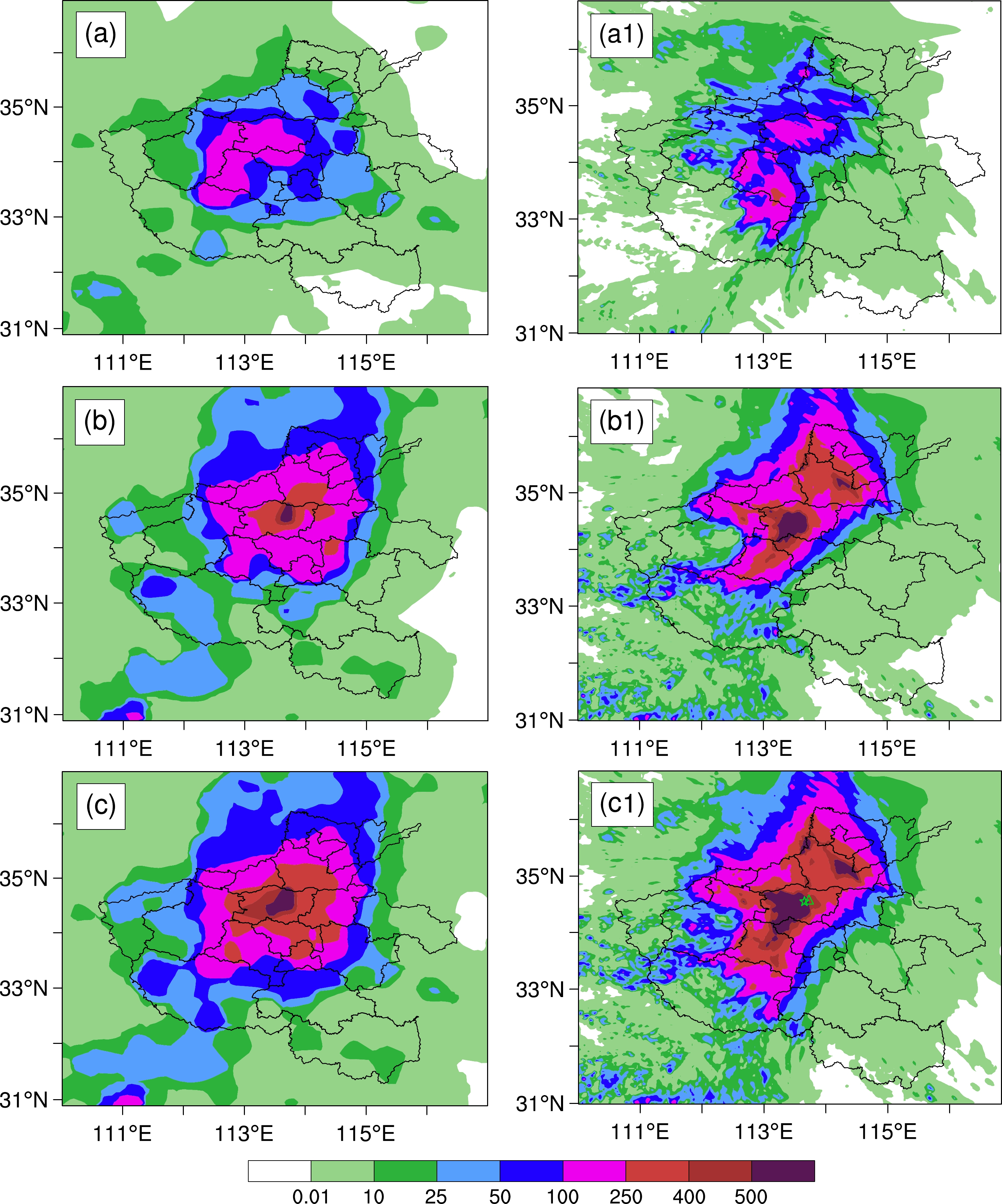
In order to verify the characteristics and evolution of the simulated rainstorm in detail, the simulated surface rainfall was first compared with observations. From 1200 UTC on 19 July to 0000 UTC on 20 July (Figs. 4a, 4a1), the observed precipitation was located in central Henan province, with 12-h precipitation exceeding 100 mm in most parts of Zhengzhou. The model generally reproduced the spatial distribution of the rainband, although the location of rainfall centers slightly deviated from observation (Fig. 4a1). From 0000 UTC on 20 July to 0000 UTC on 21 July (Figs. 4b, b1), the rainband moved northward to northern Henan province and the 24-h cumulative precipitation exceeded 250 mm in most areas of Zhengzhou. The model replicated reasonably well the spatial distribution of the rainband, especially for the rainfall cores over Zhengzhou, although it overestimated the precipitation amount over Xinxiang in the northeastern part of Henan. From 1200 UTC 19 July to 0000 UTC 21 July (Figs. 4c, c1), the distribution patterns of the rainband were similar to those of the 24-h precipitation from 0000 UTC 20 July to 0000 UTC 21 July.
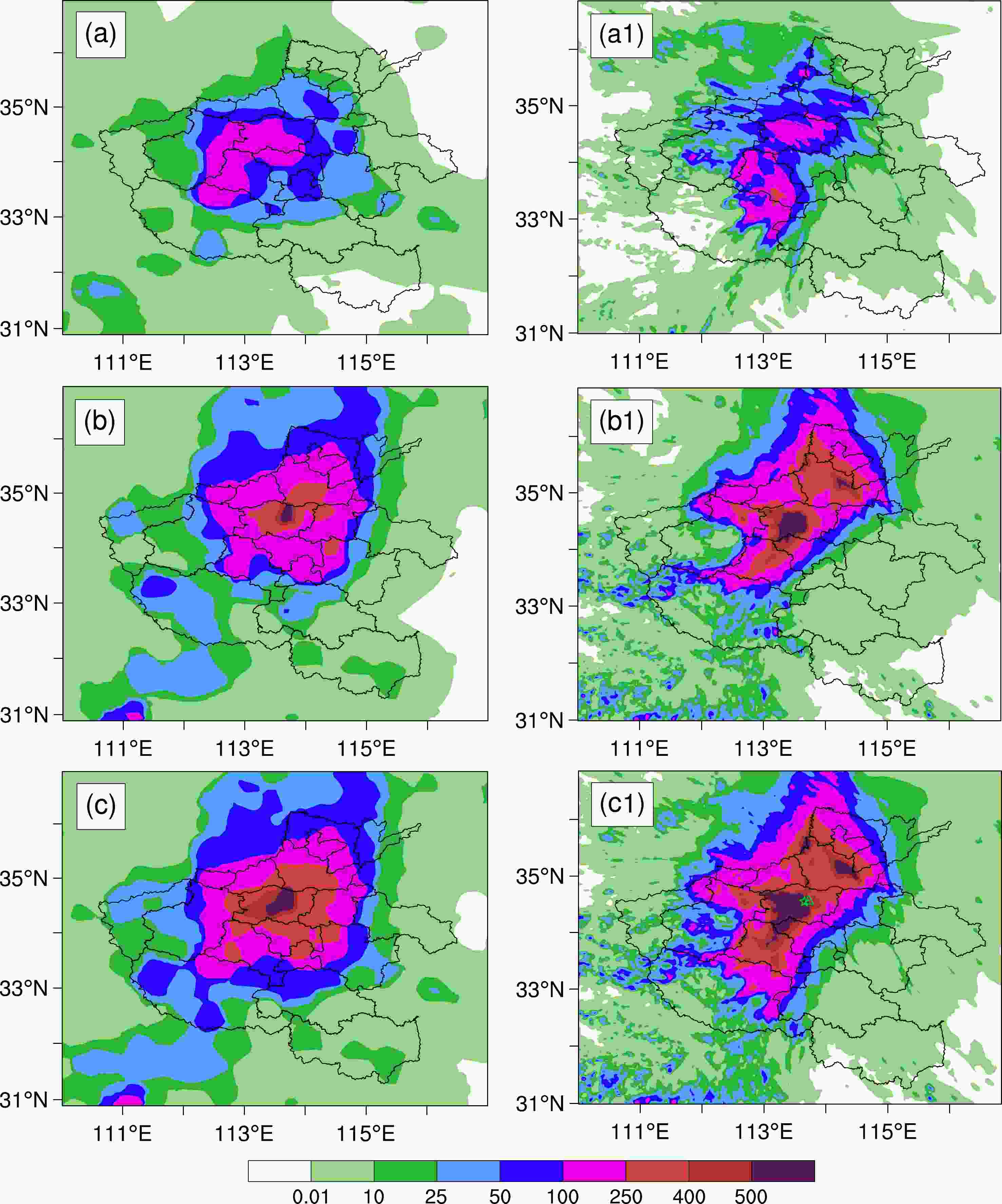
Figure 4. Distribution of (a−c) observed and (a1−c1) simulated cumulative precipitation (units: mm) (a, a1) from 1200 UTC on 19 July to 0000 UTC on 20 July 2021; (b, b1) from 0000 UTC on 20 July to 0000 UTC on 21 July; (c, c1) from 1200 UTC on 19 July to 0000 UTC on 21 July. The green triangle and star in (c1) indicate the locations where maximum hourly rainfall was observed and simulated.
Figure 3b shows the time series of hourly rainfall rates at the station where the maximum hourly rainfall was observed or simulated (indicated by the green triangle and star in Fig. 4c1). From observation, the peak hourly rainfall occurred from 0800 to 0900 UTC on 20 July, with an hourly rainfall rate of 201.9 mm h−1. The corresponding simulated peak value of 157.7 mm h−1 took place from 0730 to 0830 UTC on 20 July, which was 0.5 h earlier than observation. Deviations between the observed and simulated results were obvious in the late period of precipitation. For example, the simulated hourly rainfall rates during 1000–1800 UTC on 20 July were higher than observation. Overall, despite certain deficiencies, the WRF model could basically reproduce the spatial distribution and temporal evolution of the heavy rainstorm, especially the rainfall centers in Zhengzhou.
-
Since the strongest rainfall occurred in Zhengzhou from 0800 to 0900 UTC on 20 July, the evolution of radar reflectivity during the heavy precipitation period was analyzed and verified. At 0700 UTC (Figs. 5a), the observed convective clouds were located in Zhengzhou, with trailing stratiform clouds appearing on their north side. At 0800 UTC and 0900 UTC (Figs. 5b and 5c), the convective cells over Zhengzhou barely moved and stayed quasi-stationary, which may be the reason that extreme precipitation occurred in Zhengzhou during this period. From the simulation results (Figs. 5a1−c1), the model generally replicated the distribution and development of radar echoes, including the quasi-stationary convective cells in Zhengzhou and the trailing stratiform clouds on their north side. The differences are that the simulated convective cells occurred 0.5 h earlier than the observed, which is consistent with the time lag of maximum hourly rainfall in Fig. 3b. In addition, the model overestimated the radar reflectivity in northern Luoyang and eastern Xinxiang, which was also in line with the spatial distribution errors of rainfall in Fig. 4.
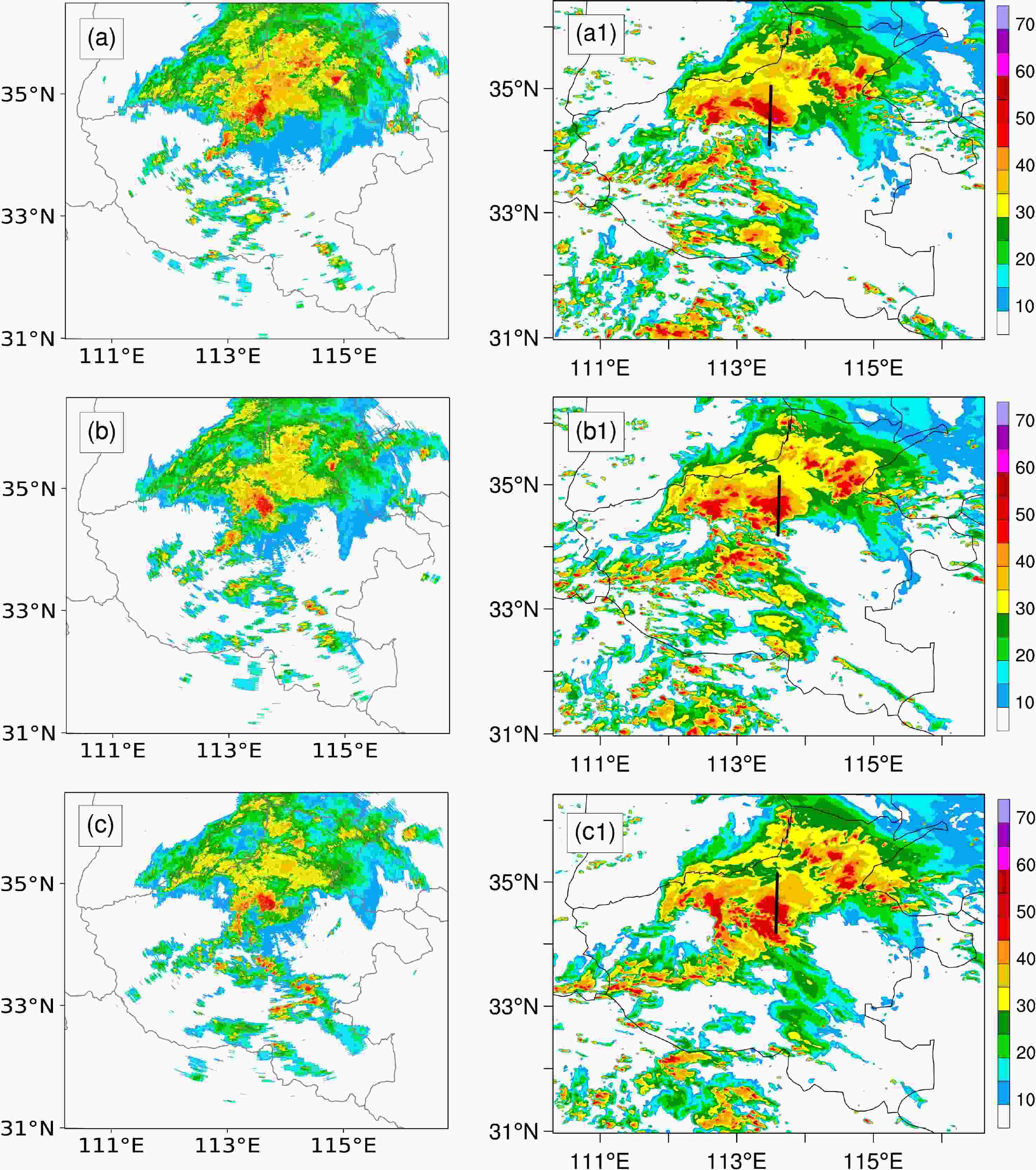
Figure 5. Observed (a−c) and simulated (a1−c1) radar reflectivity (units: dBZ) at (a) 0700 UTC, (b) 0800 UTC, and (c) 0900 UTC on 20 July 2021. The simulated data was 0.5 h earlier than observation. The black lines denote the locations of cross sections in Fig. 6.
The corresponding vertical structures of radar reflectivity are shown in Fig. 6. The observed radar reflectivity was missing in upper levels because the convective cells were too close to the radar. It can be seen that the model basically captured the structural characteristics of the observed convective cells, including the echo height and the intensity. The echoes with reflectivity greater than 45 dBZ extended to the height of 14 km, and the maximum reflectivity reached 55 dBZ at 0800 UTC on 20 July, which was consistent with the peak hourly rainfall at Zhengzhou during this period.
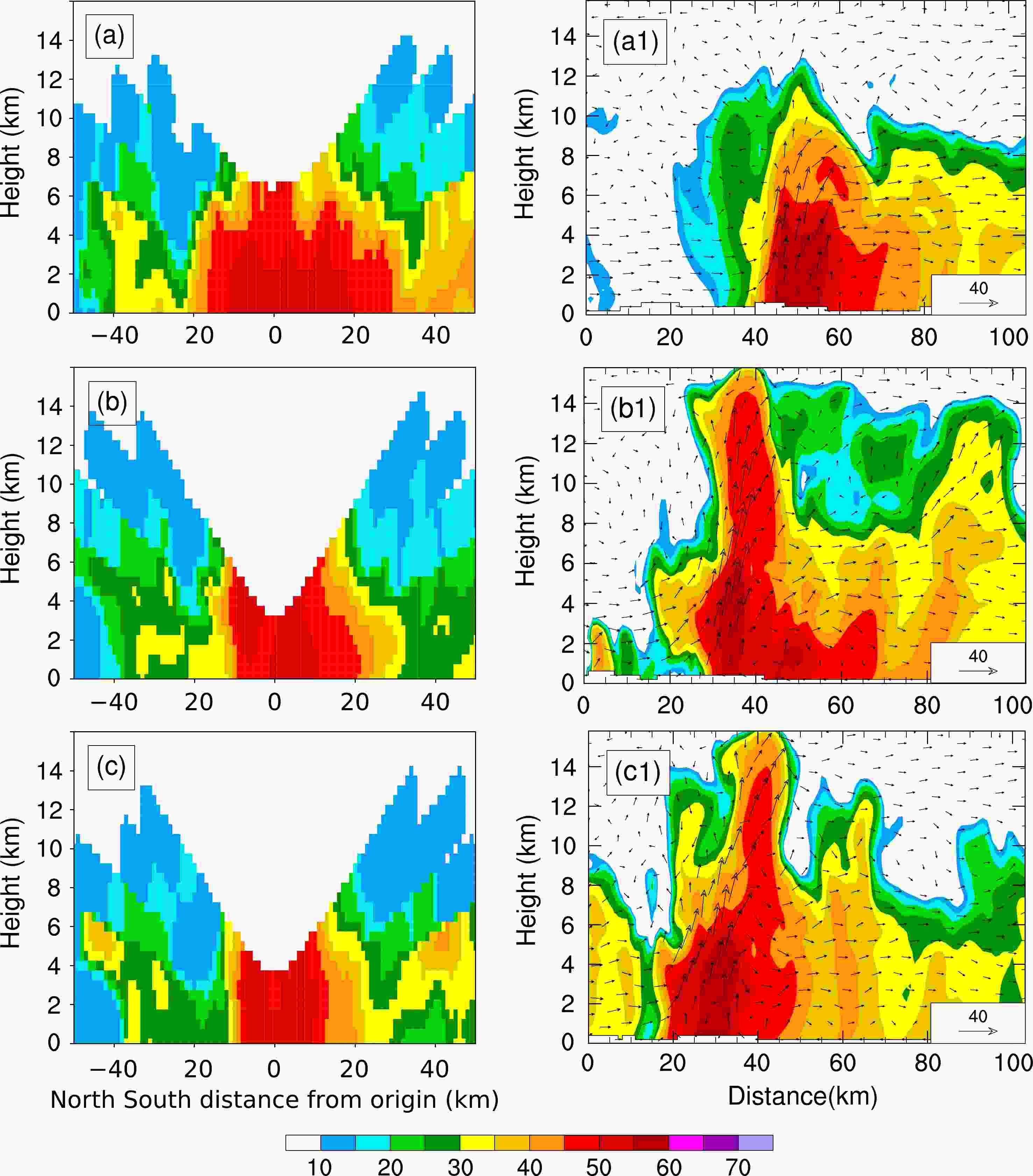
Figure 6. Vertical cross sections of observed (a−c) and simulated (a1−c1) radar reflectivity (shaded, units: dBZ) and wind field (vectors, units: m s−1) at (a) 0700 UTC, (b) 0800 UTC, and (c) 0900 UTC on 20 July 2021. The simulated data was 0.5 h earlier than observation. The radar station is located at x = 0 km in (a–c).
-
In addition to precipitation and radar reflectivity, the simulated mesoscale environmental conditions, including dynamical and thermodynamic fields, were also verified with the ERA5 reanalysis data. Generally, the occurrence of heavy rainfall in Henan was closely related to the establishment and slow northward movement of a vortex at 700 hPa. At 0000 UTC on 19 July (Fig. 7a), the vortex was located in the south of Henan, and Henan was dominated by the southeasterly air flow with moisture convergence centers in the western mountainous areas. At 0000 UTC on 20 July (Fig. 7b), the vortex moved northward to central Henan province, and strong moisture convergence existed near Zhengzhou. At 0000 UTC on 21 July (Fig. 7c), both the vortex and moisture convergence centers continued to move northward, and Henan was dominated by southerly to southwesterly winds. The location and northward movement of the vortex at 700 hPa were reproduced well by the model, and the centers of moisture convergence were also consistent with the reanalysis data, indicating that the simulation can capture the mesoscale dynamic and thermodynamic environment of the rainstorm.
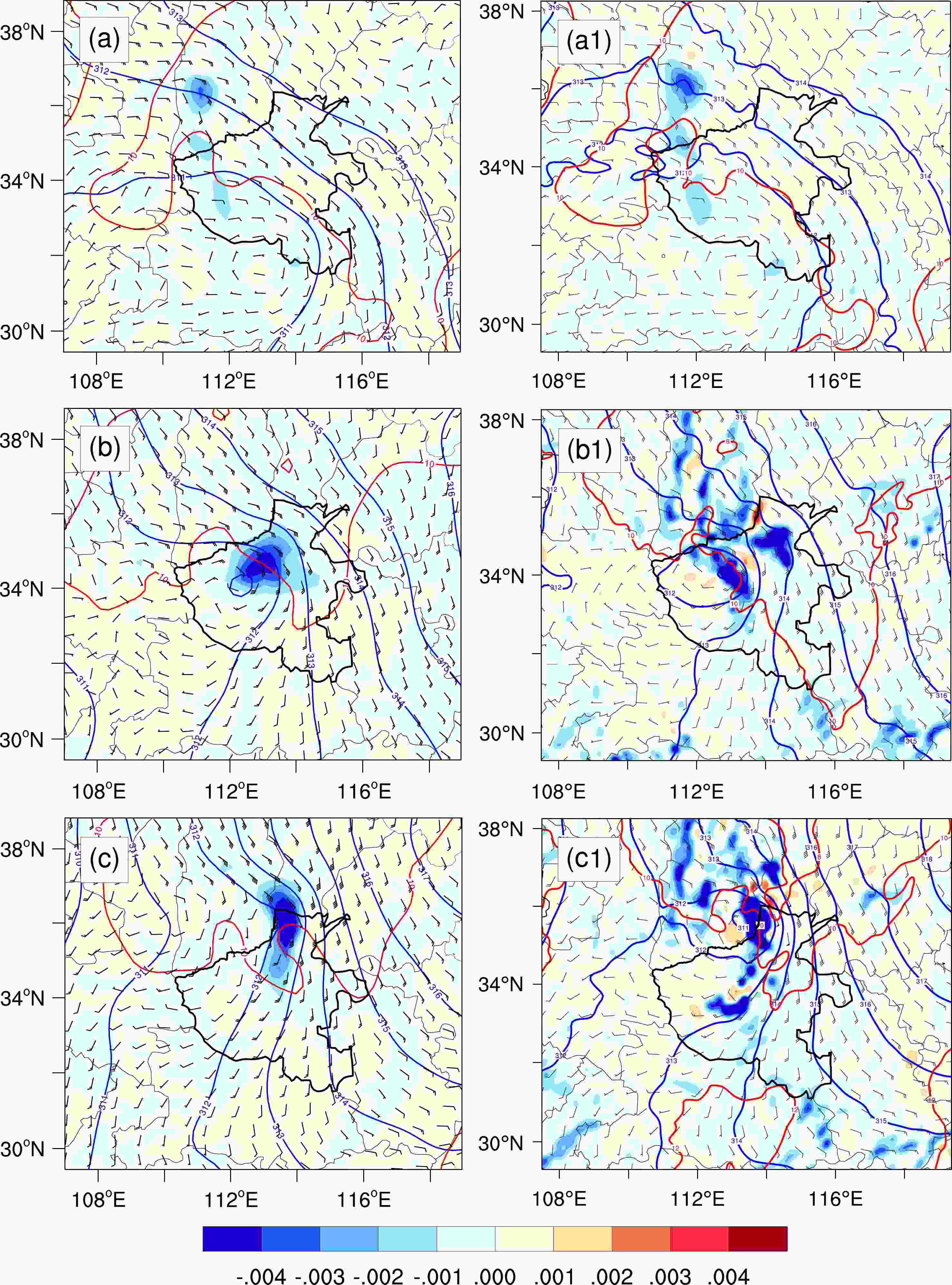
Figure 7. Mesoscale environmental fields derived from (a–c) ERA5 data and (a1–c1) simulation, with geopotential height (blue contours, units: dagpm), temperature (red contours, units: °C), wind field (barbs, full bar denotes 4 m s−1) at 700 hPa, and vertical integral of divergence of water vapor flux (shading, units: kg m−2 s−1) at (a, a1) 0000 UTC on 19 July, (b, b1) 0000 UTC on 20 July, and (c, c1) 0000 UTC on 21 July, respectively.
-
From the analysis above, the model generally reproduced the spatial and temporal distribution of the precipitation, the convective systems producing the rainstorm, and the mesoscale dynamical and thermodynamic environment. Therefore, the simulation data could be used to analyze the PE of the heavy rainfall in the following subsections.
-
Figure 8 shows the spatial distribution of surface rainfall rate, LSPE, and CMPE during the different stages of precipitation. In general, the regions with high LSPE and CMPE corresponded to the regions of heavy precipitation. For example, at 1200 UTC on 19 July (Figs. 8a−c), rainfall mainly occurred in the south of Zhengzhou and Shangqiu, showing a northwest–southeast zonal distribution. The distributions of LSPE and CMPE showed similar patterns to surface rainfall, and CMPE was greater than LSPE. At 2100 UTC on 19 July (Figs. 8a1−c1), as the rainband moved to the central Henan province, the corresponding LSPE and CMPE also showed similar distribution patterns. It should be noted that the relationship between PE and rainfall rate was not linear with one-to-one correspondence. Based on the formulas of LSPE and CMPE, the regions of weak precipitation may have weak moisture convergence and surface evaporation, which may lead to relatively high LSPE to some extent.

Figure 8. Distribution of (a–a2) hourly rainfall (units: mm), (b–b2) LSPE, and (c–c2) CMPE at (a–c)1200 UTC on 19 July; (a1–c1) 2100 UTC on 19 July; (a2–c2) 1000 UTC on 20 July, respectively. The black box indicates the area of regional average
-
Figure 9 shows the time series of the area-averaged (34.3º–34.8ºN, 113º–114.1ºE) hourly rainfall rate, LSPE, and CMPE. As seen from Fig. 9a, the observed hourly rainfall rate (black line) showed a fluctuating upward trend staring from 0000 UTC 19 July, with a peak of 29 mm h−1 at 0900 UTC on 20 July, which was similar to the trend of hourly precipitation seen at Zhengzhou station in Fig. 3b. The corresponding simulations (red line) showed similar variation trends, with a maximum value of 27 mm h−1 at 1000 UTC on 20 July. Thus, the simulation generally replicated the evolution and magnitude of the observed precipitation from the perspective of regional average and could be used to calculate LSPE and CMPE. From Fig. 9b, it was found that CMPE was always greater than LSPE, and the average LSPE and CMPE were about 33.34% and 58.13%, respectively. According to the studies by Mao et al. (2018), the average LSPE and CMPE for the “7.21” rainstorm in Beijing were 36.09% and 60.66% in the warm sector precipitation stage and were 32.12% and 54.02% in the cold frontal precipitation stage, respectively. The average LSPE and CMPE of the “21.7” Henan rainstorm were between the values of warm-sector and cold frontal precipitation during the “7.21” rainstorm. It was noteworthy that the highest LSPE and CMPE were 58.26% and 88.54%, respectively, at 0300 UTC on 20 July, although the strongest hourly rainfall occurred at 0900 UTC 20 July.
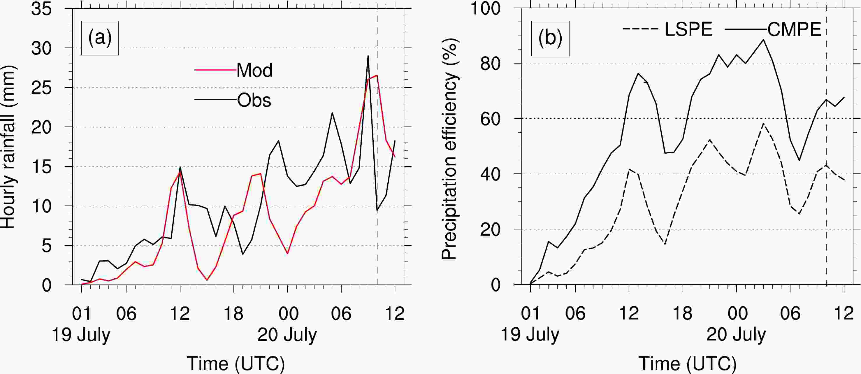
Figure 9. (a) Time series of average hourly precipitation (units: mm h−1); (b) Time series of LSPE and CMPE (units: %). Area average is over the range of the black box in Fig. 8.
-
To determine the key physical factors influencing LSPE, the numerator and denominator terms of LSPE were analyzed (Figs. 10a, 10c). In general, the
$ {Q}_{\mathrm{W}\mathrm{V}\mathrm{F}} $ was the main positive contributor to$ {P}_{\mathrm{s}} $ , accounting for 86.75%. The contribution rates of the other terms were relatively small (Table 3). Therefore,$ {Q}_{\mathrm{W}\mathrm{V}\mathrm{F}} $ had a significant impact on the surface rainfall. From the denominator term of LSPE (Fig. 10c), the water vapor flux convergence$H\left({Q}_{\mathrm{W}\mathrm{V}\mathrm{F}}\right)$ ${Q}_{\mathrm{W}\mathrm{V}\mathrm{F}} $ played a key role in the supply of water vapor, accounting for 48.19%, followed by the local atmospheric drying$H\left({Q}_{\mathrm{W}\mathrm{V}\mathrm{T}}\right)$ ${Q}_{\mathrm{W}\mathrm{V}\mathrm{T}} $ , contributing 36.49%.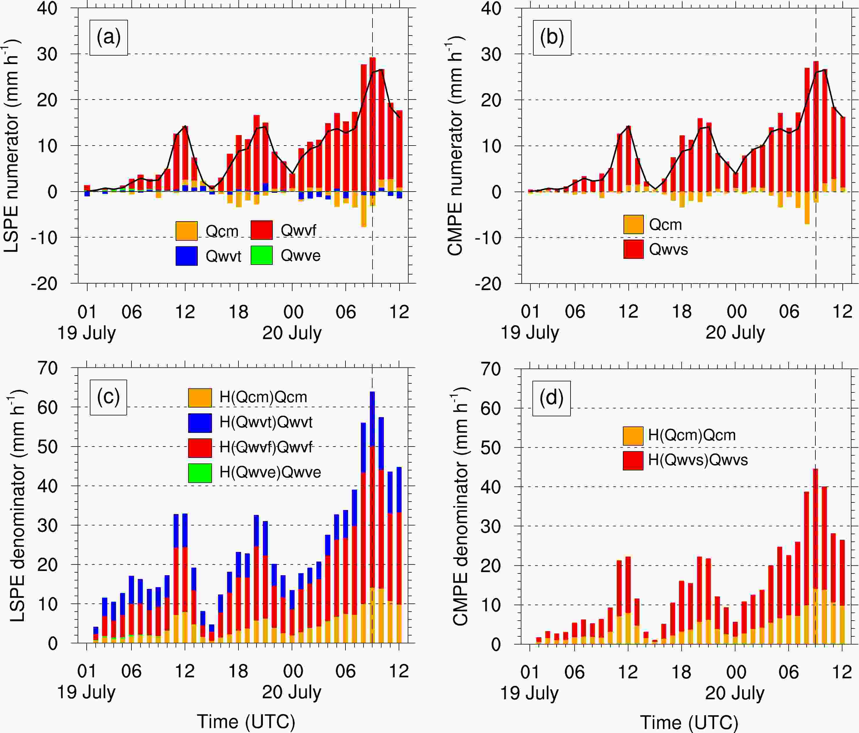
Figure 10. Time series of area-averaged numerator terms (units: mm h−1) of (a) LSPE and (b) CMPE; Time series of area-averaged denominator terms (units: mm h−1) of (c) LSPE and (d) CMPE. The black lines in (a) and (b) denote the surface rainfall rate. Area average is over the range of the black box in Fig. 8.
Terms Contribution rates (%) LSPE numerator CMPE numerator LSPE denominator CMPE denominator $ {Q}_{\mathrm{W}\mathrm{V}\mathrm{F}} $ 86.75 − 48.19 − $ {Q}_{\mathrm{W}\mathrm{V}\mathrm{T}} $ 7.30 − 36.49 − $ {Q}_{\mathrm{C}\mathrm{M}} $ –3.31 –3.31 13.51 34.28 $ {Q}_{\mathrm{W}\mathrm{V}\mathrm{E}} $ 9.26 − 1.81 − $ {Q}_{\mathrm{W}\mathrm{V}\mathrm{S}} $ − 103.31 − 65.72 Table 3. Contribution rates of different terms in LSPE and CMPE.
To understand the influence of
$ {Q}_{\mathrm{W}\mathrm{V}\mathrm{F}} $ on LSPE,$ {Q}_{\mathrm{W}\mathrm{V}\mathrm{F}} $ can be further decomposed into (a) the water vapor convergence ($ \mathrm{Q}\mathrm{G}\mathrm{R}\mathrm{A}\mathrm{D}\mathrm{V} $ ) and (b) the water vapor advection ($ \mathrm{V}\mathrm{G}\mathrm{R}\mathrm{A}\mathrm{D}\mathrm{Q} $ ):It is clear from Fig. 11a that
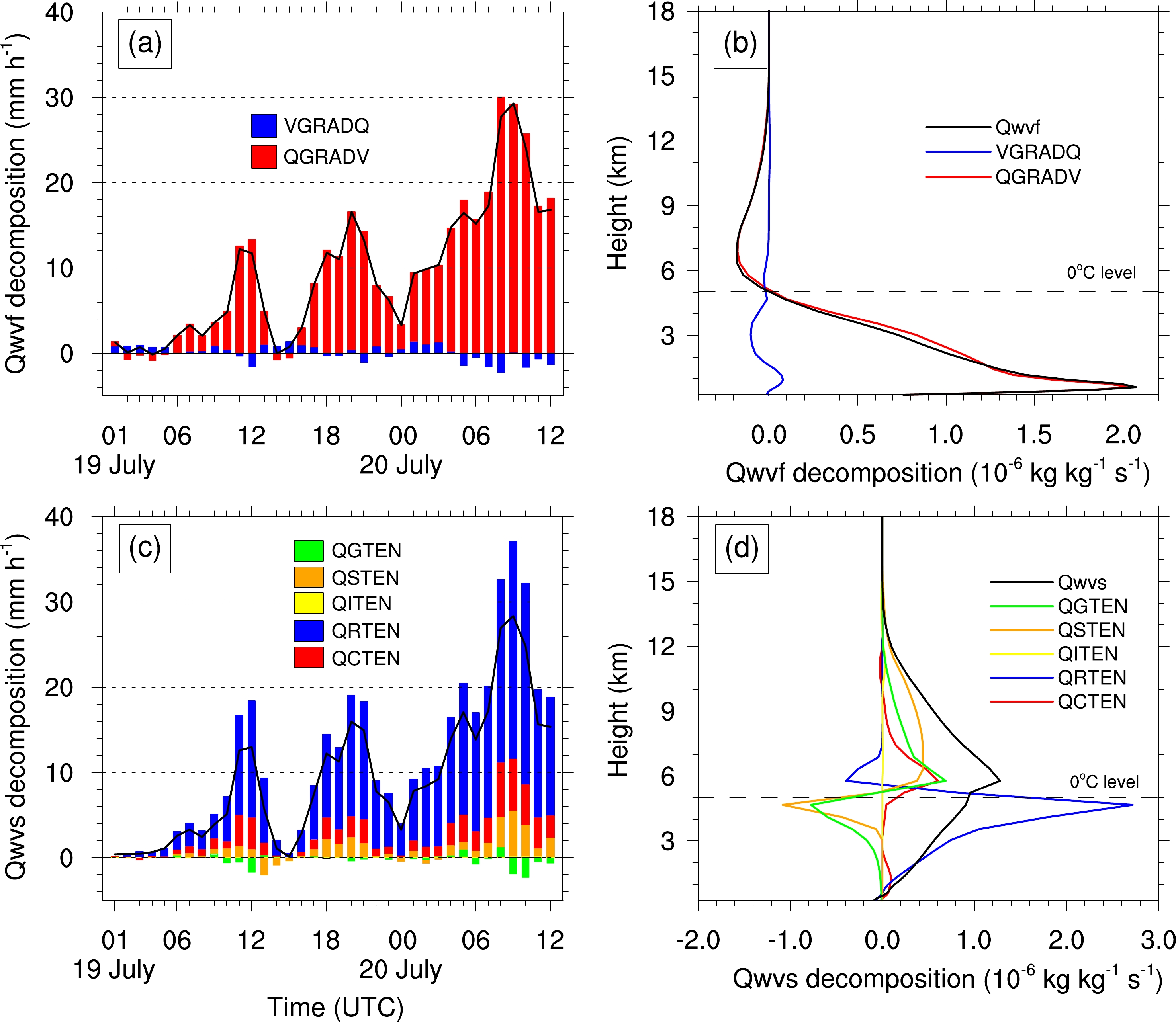
$ {Q}_{\mathrm{W}\mathrm{V}\mathrm{F}} $ was almost completely contributed by$ \mathrm{Q}\mathrm{G}\mathrm{R}\mathrm{A}\mathrm{D}\mathrm{V} $ , and the contribution of$ \mathrm{V}\mathrm{G}\mathrm{R}\mathrm{A}\mathrm{D}\mathrm{Q} $ was very small.$ \mathrm{Q}\mathrm{G}\mathrm{R}\mathrm{A}\mathrm{D}\mathrm{V} $ reached a maximum value at 0800 UTC, when heavy precipitation happened, indicating that strong convergence of water vapor ($ \mathrm{Q}\mathrm{G}\mathrm{R}\mathrm{A}\mathrm{D}\mathrm{V} $ > 0) played a significant role in the formation of heavy rainfall. Furthermore, the vertical profiles of the non-integral$ \mathrm{Q}\mathrm{G}\mathrm{R}\mathrm{A}\mathrm{D}\mathrm{V} $ and$ \mathrm{V}\mathrm{G}\mathrm{R}\mathrm{A}\mathrm{D}\mathrm{Q} $ are given in Fig. 11b. Water vapor convergence ($ \mathrm{Q}\mathrm{G}\mathrm{R}\mathrm{A}\mathrm{D}\mathrm{V} $ > 0) occurred below the 0°C layer, with the strongest convergence near the surface, while moisture divergence ($ \mathrm{Q}\mathrm{G}\mathrm{R}\mathrm{A}\mathrm{D}\mathrm{V} $ < 0) occurred above the 0°C layer, with its peak between the heights of 6−7 km. The advection of water vapor ($ \mathrm{V}\mathrm{G}\mathrm{R}\mathrm{A}\mathrm{D}\mathrm{Q} $ ) mainly occurred below 6 km, with moist advection ($ \mathrm{V}\mathrm{G}\mathrm{R}\mathrm{A}\mathrm{D}\mathrm{Q} $ > 0) extending from the ground to 1.5 km and dry advection ($ \mathrm{V}\mathrm{G}\mathrm{R}\mathrm{A}\mathrm{D}\mathrm{Q} $ < 0) between 1.5−6 km, indicating that there was intrusion of dry and cold air in the lower and middle troposphere.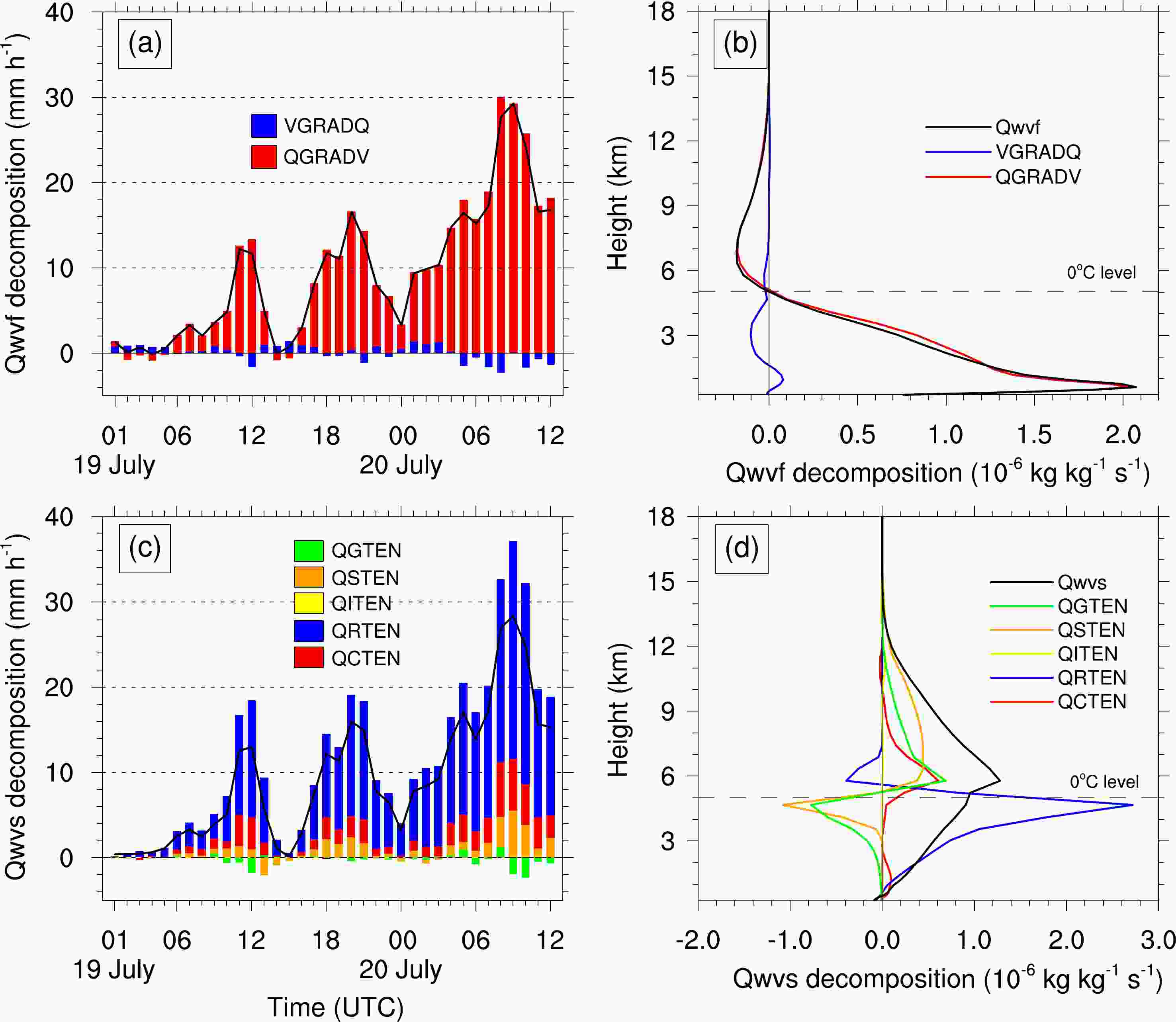
Figure 11. (a) Time series and (b) vertical profiles of area-averaged
$ \mathrm{Q}\mathrm{G}\mathrm{R}\mathrm{A}\mathrm{D}\mathrm{V} $ (red bar and line),$ \mathrm{V}\mathrm{G}\mathrm{R}\mathrm{A}\mathrm{D}\mathrm{Q} $ (blue bar and line), and$ {Q}_{\mathrm{W}\mathrm{V}\mathrm{F}} $ (black line); (c) Time series and (d) vertical profiles of area-averaged tendency of hydrometeors, including cloud water ($ \mathrm{Q}\mathrm{C}\mathrm{T}\mathrm{E}\mathrm{N} $ , red bar and line), rainwater ($ \mathrm{Q}\mathrm{R}\mathrm{T}\mathrm{E}\mathrm{N} $ , blue bar and line), ice crystal ($ \mathrm{Q}\mathrm{I}\mathrm{T}\mathrm{E}\mathrm{N} $ , yellow bar and line), snow ($ \mathrm{Q}\mathrm{S}\mathrm{T}\mathrm{E}\mathrm{N} $ , orange bar and line), graupel ($ \mathrm{Q}\mathrm{G}\mathrm{T}\mathrm{E}\mathrm{N} $ , green bar and line), and$ {Q}_{\mathrm{W}\mathrm{V}\mathrm{S}} $ (black line) . The black dotted line represents the height of the 0°C layer. Area average is over the range of the black box in Fig. 8. -
The impacts of physical factors on CMPE are represented in Figs. 10b and d. It can be found that the mean contribution rates of
$ {Q}_{\mathrm{W}\mathrm{V}\mathrm{S}} $ and$ {Q}_{\mathrm{C}\mathrm{M}} $ to$ {P}_{\mathrm{s}} $ were 103.31% and –3.31%, respectively, while$ H\left({Q}_{\mathrm{W}\mathrm{V}\mathrm{S}}\right){Q}_{\mathrm{W}\mathrm{V}\mathrm{S}} $ and$ {H(Q}_{\mathrm{C}\mathrm{M}}){Q}_{\mathrm{C}\mathrm{M}} $ accounted for 65.72% and 34.28%, respectively, in the denominator terms of CMPE (Fig. 10d). Clearly,$ {Q}_{\mathrm{W}\mathrm{V}\mathrm{S}} $ was the key physical factor that influenced CMPE.The net consumption of water vapor by microphysical processes (
$ {Q}_{\mathrm{W}\mathrm{V}\mathrm{S}} $ ) is equal to the sum of the net increase in hydrometeors ($ \mathrm{Q}\mathrm{C}\mathrm{T}\mathrm{E}\mathrm{N} $ ,$ \mathrm{Q}\mathrm{R}\mathrm{T}\mathrm{E}\mathrm{N} $ ,$ \mathrm{Q}\mathrm{I}\mathrm{T}\mathrm{E}\mathrm{N} $ ,$ \mathrm{Q}\mathrm{S}\mathrm{T}\mathrm{E}\mathrm{N} $ ,$ \mathrm{Q}\mathrm{G}\mathrm{T}\mathrm{E}\mathrm{N} $ ), so we analyzed the tendency of hydrometeors to indirectly study the impacts of$ {Q}_{\mathrm{W}\mathrm{V}\mathrm{S}} $ on CMPE. In terms of magnitude, the$ \mathrm{Q}\mathrm{R}\mathrm{T}\mathrm{E}\mathrm{N} $ term had the greatest influence on$ {Q}_{\mathrm{W}\mathrm{V}\mathrm{S}} $ , followed by$ \mathrm{Q}\mathrm{C}\mathrm{T}\mathrm{E}\mathrm{N} $ and$ \mathrm{Q}\mathrm{S}\mathrm{T}\mathrm{E}\mathrm{N} $ (Fig. 11c), revealing that most of the consumed water vapor was transformed to cloud water between 5–7 km and snow and graupel between 5–10 km, and then converted to raindrops near the 0°C layer through melting and collision-coalescence (Fig. 11d).Furthermore, we decompose
$ \mathrm{Q}\mathrm{R}\mathrm{T}\mathrm{E}\mathrm{N} $ to study the impact of rain-related microphysical processes on CMPE. The calculation of$ \mathrm{Q}\mathrm{R}\mathrm{T}\mathrm{E}\mathrm{N} $ is as follows:As seen from Fig. 12a, rainwater was mainly formed through the accretion of cloud water (
$ \mathrm{P}\mathrm{R}\mathrm{A} $ ), followed by melting of snow ($ \mathrm{P}\mathrm{S}\mathrm{M}\mathrm{L}\mathrm{T} $ ) and graupel ($ \mathrm{P}\mathrm{G}\mathrm{M}\mathrm{L}\mathrm{T} $ ). The primary sink of rainwater was evaporation ($ \mathrm{P}\mathrm{R}\mathrm{E} $ ). From the vertical profiles, during 0000–0100 UTC on 20 July (Fig. 12b), rain mixing ratio was mainly contributed by$ \mathrm{P}\mathrm{S}\mathrm{M}\mathrm{L}\mathrm{T} $ at about 4–5 km, followed by$ \mathrm{P}\mathrm{R}\mathrm{A} $ below the melting level. During 0800–0900 UTC, when the heavy rainfall occurred (Fig. 12b1), the conversion rates of$ \mathrm{P}\mathrm{G}\mathrm{M}\mathrm{L}\mathrm{T} $ and$ \mathrm{P}\mathrm{R}\mathrm{A} $ increased significantly and became the main contributors to rain mass. The budget of rain number concentration showed similar results (Figs. 12c–c1). During the heavy precipitation period, a great number of raindrops were produced by auto-conversion from cloud droplets ($ \mathrm{N}\mathrm{P}\mathrm{R}\mathrm{C}1 $ ) between 5–8 km and between 2–3 km. Near the melting layer, rain number concentration was mainly contributed by$ \mathrm{P}\mathrm{G}\mathrm{M}\mathrm{L}\mathrm{T} $ . The number concentration of rain decreased rapidly between 4–5 km through self-collection ($ \mathrm{N}\mathrm{R}\mathrm{A}\mathrm{G}\mathrm{G} $ ). The budget analysis suggested that$ \mathrm{P}\mathrm{R}\mathrm{A} $ and$ \mathrm{P}\mathrm{G}\mathrm{M}\mathrm{L}\mathrm{T} $ were the main contributors to rain mixing ratio and number concentration during the heavy precipitation stage. In the Morrison microphysical scheme,$ \mathrm{P}\mathrm{R}\mathrm{A} $ was proportional to the mixing ratios of cloud water and rainwater. During the heavy precipitation period, both cloud water and rainwater mixing ratios increased significantly, thus the production rate of$ \mathrm{P}\mathrm{R}\mathrm{A} $ also increased.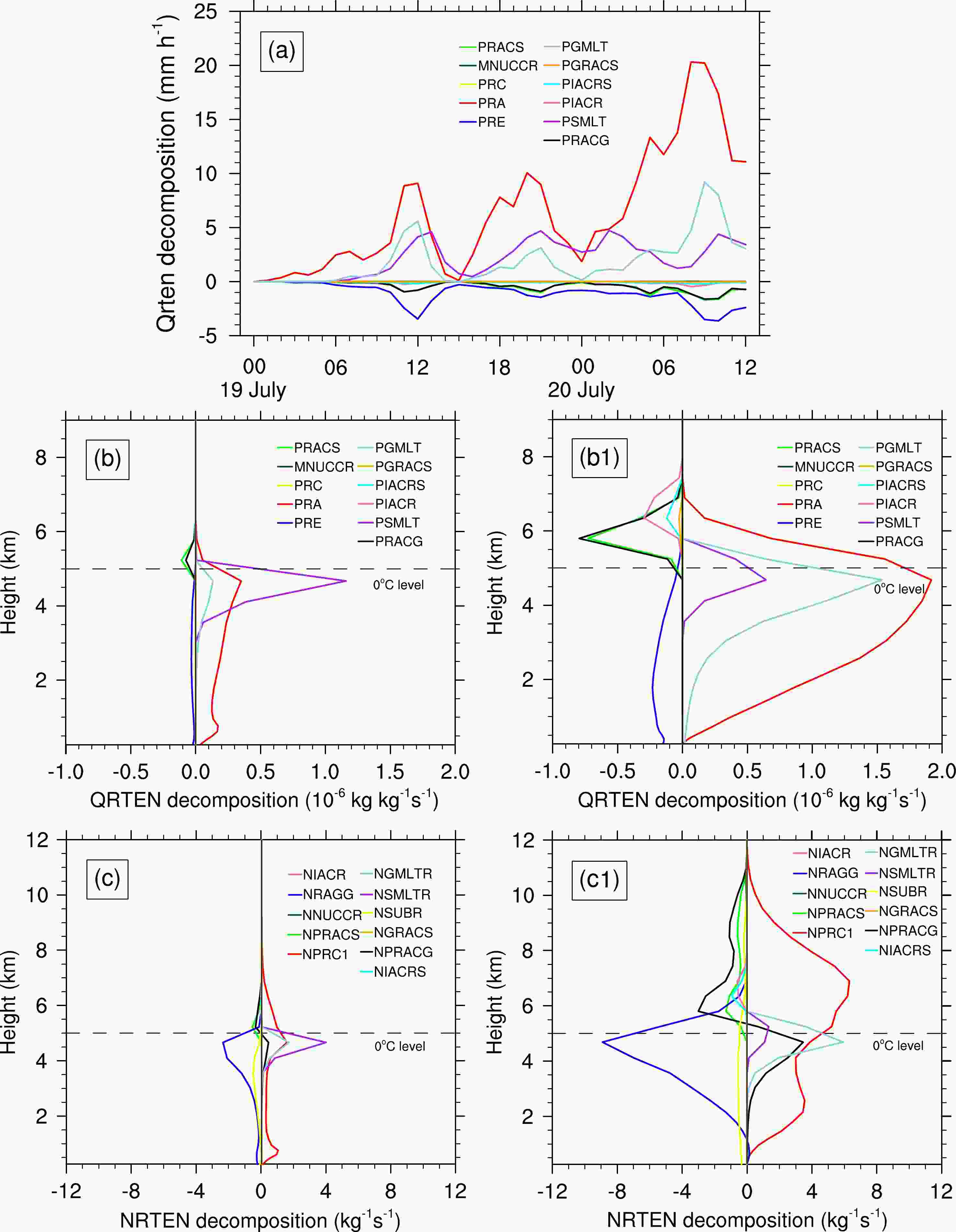
Figure 12. (a) Time series and vertical profiles of source and sink terms of (b, b1) rain mixing ratio (
$ \mathrm{Q}\mathrm{R}\mathrm{T}\mathrm{E}\mathrm{N} $ ) and (c, c1) rain number concentration ($ \mathrm{N}\mathrm{R}\mathrm{T}\mathrm{E}\mathrm{N} $ ). (b, c) are averaged during 0000–0100 UTC on 20 July, (b1, c1) are averaged during 0800–0900 UTC on 20 July. -
From the analysis above, it was found that water vapor convergence was the key physical factor in LSPE, and the rain-related source terms were crucial in CMPE. In this section, the possible mechanisms of LSPE and CMPE are further explored.
-
Figure 13 shows the horizontal and vertical distributions of water vapor flux divergence derived from ERA5 data. Figure 2 illustrates that water vapor was transported by a strong southeasterly air flow from the East China Sea to Henan under the influence of the subtropical high and Typhoon In-Fa (2021). Meanwhile, the southerly air flow of Typhoon Cempaka (2021) also transported water vapor to Henan. The two water vapor transport channels converged in Zhengzhou, providing sufficient moisture for the heavy rainstorm. From Fig. 13, it can be seen that water vapor was blocked by the Taihang and Funiu Mountains in western Henan province, and strong moisture convergence formed on the windward slope in front of the mountain. From the vertical cross section, it can be seen that at 0000 UTC on 20 July the moisture convergence extended from near the ground to the level of 500 hPa, with the strongest convergence located at 925 hPa.

Figure 13. Vertical integral of divergence of moisture flux (blue shading, units: kg m−2 s−1), wind field at 850 hPa (barbs, full barb denotes 4 m s−1), and terrain height (gray shading, units: m) at (a) 0000 UTC and (b) 1200 UTC on 20 July 2021; Zonal–vertical distribution of divergence of moisture flux (shading, units: 10−7 kg m−2 s−1 hPa−1) and wind field (arrows, units: m s−1) along 34.6°N at (c) 0000 UTC and (d) 1200 UTC. The red line indicates the location of cross sections.
A sensitivity experiment was performed to further examine the blocking of moisture by the Funiu and Taihang Mountains. In the sensitivity experiment, the terrain height of the mountainous area (32.5°–36.0°N, 110.5°–114.0°E) in western Henan province was modified to half of the original height. The simulation results showed that the rainfall center in the sensitivity experiment moved northward to Jiaozuo city and the maximum accumulated precipitation was about 756 mm, which was much lower than that simulated in the control experiment (about 1041 mm, figure omitted). It was found that the moisture convergence over Zhengzhou in the sensitivity experiment was slightly weaker than that in the control experiment, suggesting the topographic blocking of the Taihang and Funiu Mountains enhanced moisture convergence in Zhengzhou and prompted heavy rainfall. The blocking effect of mountains and its role in the convective initiation in the southwest of Zhengzhou are fully discussed by Yin et al. (2022).
-
To understand the probable mechanism of CMPE, a diagnostic study of environmental and microphysical variables was performed. It is shown in Fig. 14a that there was a high relative humidity (RH) layer between 4–8 km over Zhengzhou, which may be the results of large-scale vapor transport and updrafts induced by local topography. RH deceased significantly at about 0800–0900 UTC on 20 July when heavy rainfall happened. In terms of dynamic fields, both the updrafts and downdrafts reached their peaks at 0900−1000 UTC 20 July, and so did the mass contents of liquid water (sum of cloud water and rainwater) and ice phase particles (sum of cloud ice, snow, and graupel). From the thermodynamic fields, we found there was a negative potential temperature perturbation between 3–5 km starting from 1200 UTC on 19 July and reaching its maximum at 0000 UTC on 20 July, which may be associated with the diabatic cooling of evaporation and melting processes.

Figure 14. Time–height distribution of (a) relative humidity (units: %); (b) updraft (units: m s−1); (c) downdraft (units: m s−1); (d) mass content of liquid water (units: g kg−1); (e) mass content of ice phase particles (units: g kg−1); (f) potential temperature perturbation (units: K). The black solid line is the hourly precipitation, and the red solid lines are the 0°C and −20°C isotherms.
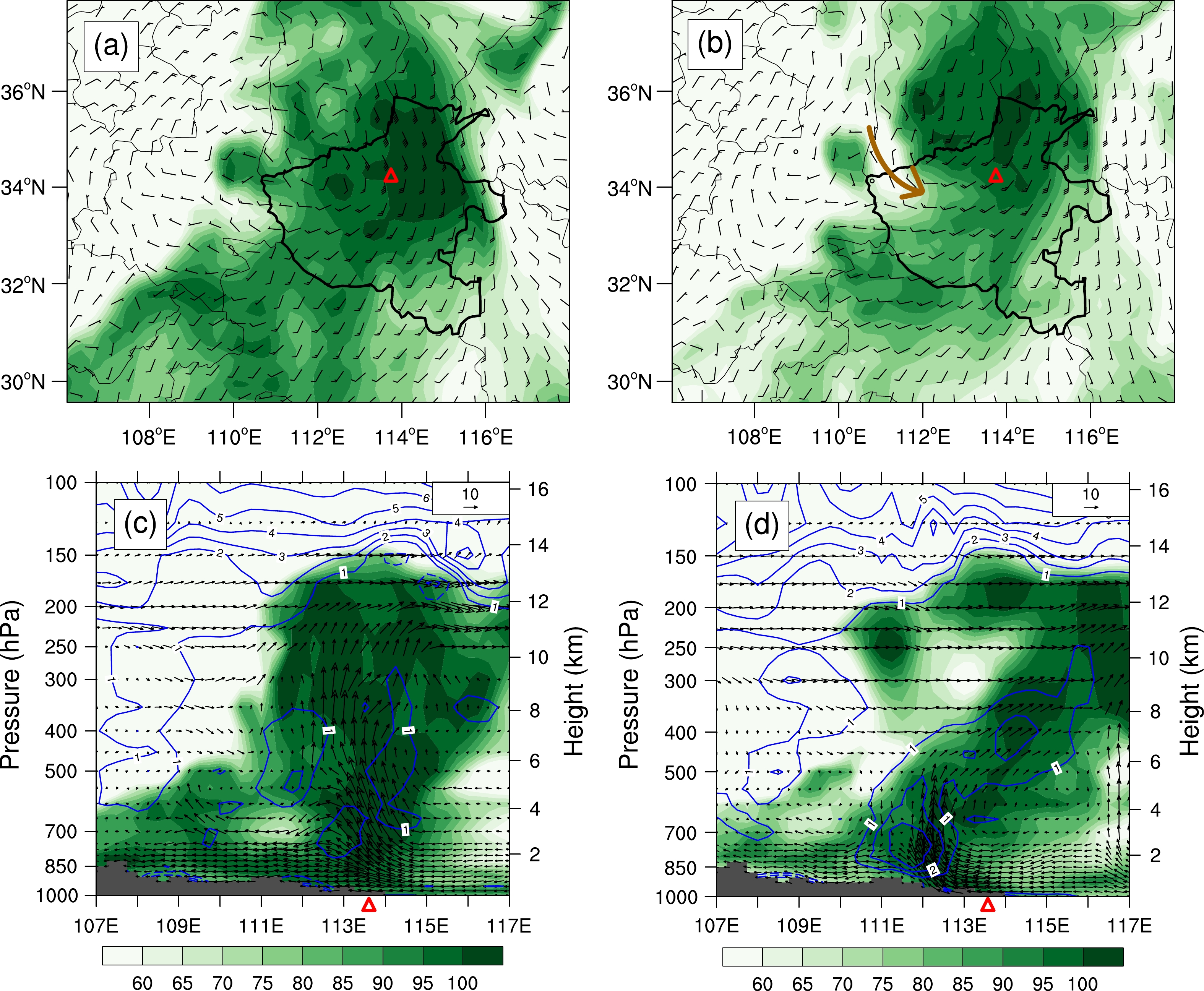
According to the studies by Browning and Golding (1995) and Browning (1997), dry intrusion is a coherent region of air descending from near-tropopause level. The dry intrusion is characterized by high potential vorticity and relatively low wet-bulb potential temperature and can lead to convective instability where it overruns the warm air. In our study, dry intrusion air is defined as the air with RH less than 60% (Yao et al., 2007). Figure 15 shows the wind field and RH at 500 hPa derived from ERA5 reanalysis data. At 0000 UTC on 20 July (Fig. 15a), the low vortex at 500 hPa was located in western Henan province and Zhengzhou is controlled by the southwesterly flow with RH greater than 100%. At 0800 UTC, when the strong precipitation occurred (Fig. 15b), dry air (RH less than 60%) intruded from the northwestern part of the vortex into Zhengzhou (indicated by the brown arrow), and the RH over Zhengzhou decreased to 90%. The dry intrusion was also significant at 300 hPa (figure omitted). Figures 15c–d depict the zonal–vertical cross sections of RH and potential vorticity (PV) along Zhengzhou. At 0000 UTC, the low levels over Henan were dominated by easterly winds, and strong updrafts were induced by orographic lifting. The air over Zhengzhou was very moist, with RH over 100% extending from the surface to upper troposphere. Regions of high PV were mainly located above 12 km and in the middle-to-upper levels between 107°–111°E, which was a result of downward movement of high PV from the upper levels. At 0800 UTC, there was dry air intrusion in the middle and upper levels of Zhengzhou. The dry and cold air was superimposed on the warm and moist air in the lower levels, which enhanced the convective instability in Zhengzhou. Moreover, the descending of high PV from the upper troposphere interacted with the high PV in the lower levels, which promoted the development of a low vortex and also enhanced precipitation (Yao et al., 2007). The intrusion of cold and dry air also resulted in the supersaturation and condensation of water vapor, which contributed to rainfall through
$ \mathrm{P}\mathrm{R}\mathrm{A} $ .
Figure 15. (a–b) Relative humidity (shading, units: %) and wind field (barbs, full barb denotes 4 m s−1) at 500 hPa derived from ERA5 data; (c–d) Zonal–vertical distribution of relative humidity (shading, units: %), potential vorticity (blue contours, units: PUV) and wind field (vectors) along 34.9°N at (a, c) 0000 UTC and (b, d) 0800 UTC on 20 July. The red triangles denote the location of Zhengzhou.
-
An extremely heavy rainfall event that occurred in Zhengzhou, Henan province on 19−21 July 2021, was simulated using the WRF model. The LSPE and CMPE of the heavy rainfall were analyzed based on the simulation results. Then, the key physical factors that influenced LSPE and CMPE and the possible mechanisms for the heavy rainfall were explored. The main conclusions are as follows:
(1) The favorable synoptic-scale conditions of the extreme rainfall in Zhengzhou included an exceptionally northward subtropical high over Northeast Asia, a deep South Asia high over the Qinghai–Tibet Plateau, Typhoon In-Fa (2021) over the East China Sea, Typhoon Cempaka (2021) over the South China Sea, and a slow northward moving low vortex over western Henan province.
(2) Quantitative analysis of LSPE showed that water vapor flux convergence/divergence (
$ {Q}_{\mathrm{W}\mathrm{V}\mathrm{F}} $ ) played a key role in LSPE; in particular, the water vapor convergence ($ \mathrm{Q}\mathrm{G}\mathrm{R}\mathrm{A}\mathrm{D}\mathrm{V} $ > 0) was the greatest contributor to$ {Q}_{\mathrm{W}\mathrm{V}\mathrm{F}} $ , with the strongest moisture convergence occurring at 0.5 km. By analyzing the large-scale environmental conditions of the rainstorm, it was revealed that water vapor was transported by the southeasterly flow between Typhoon In-Fa (2021) and the subtropical high and the southerly wind of Typhoon Cempaka (2021). The two water vapor channels converged in Zhengzhou due to the blocking by the Taihang and Funiu Mountains in northwest Henan province, causing strong moisture convergence on the windward slope in front of the mountain, which led to high LSPE in Zhengzhou.(3) The net consumption of water vapor by microphysical processes (
$ {Q}_{\mathrm{W}\mathrm{V}\mathrm{S}} $ ) was the key factor that influenced CMPE. Budget analysis of the microphysical processes suggested that water vapor was mainly consumed to produce cloud water and ice-phase particles and then transformed to raindrops through melting of graupel and accretion of cloud water by rainwater. Analyzing the dynamic and thermodynamic environment revealed that there was dry air intrusion in the middle and upper levels over Zhengzhou during the heavy precipitation stage. The dry and cold air was superimposed on the warm and moist air in lower levels, which enhanced the convective instability. Moreover, the descent of high PV from the upper troposphere interacted with the high PV in the lower levels, which also promoted the development of a low vortex and enhanced precipitation. The intrusion of cold and dry air also resulted in the supersaturation of water vapor and prompted the condensation process, which contributed to rainfall through$ \mathrm{P}\mathrm{R}\mathrm{A} $ . The aforementioned processes are summarized in a conceptual model given in Fig. 16.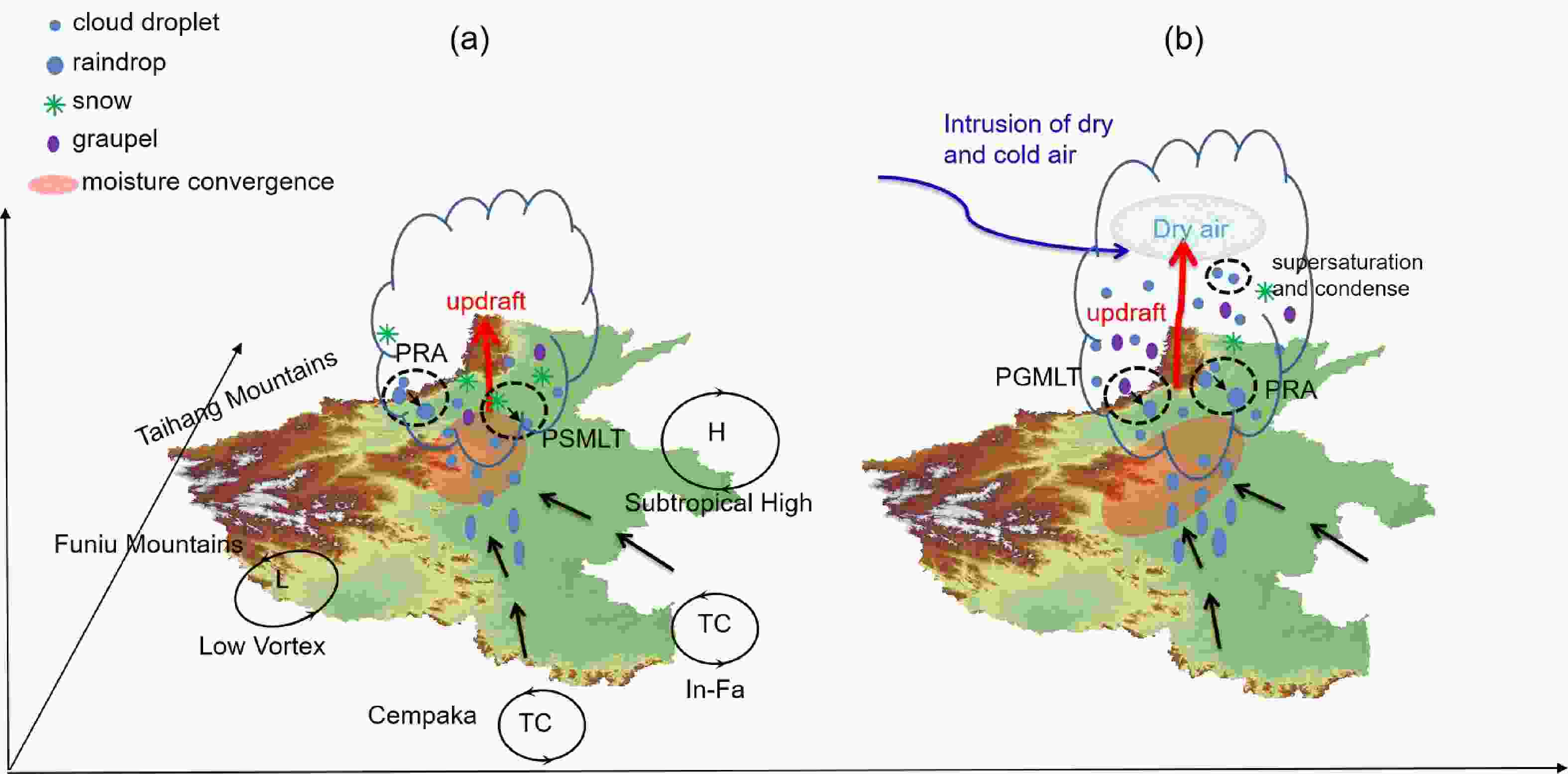
Figure 16. Conceptual model of the “21.7” Henan extremely heavy rainfall event (a) before and (b) when the heavy precipitation occurred.
In this paper, the key influencing factors of LSPE and CMPE and possible mechanisms of the “21.7” Henan extremely heavy rainfall event were explored, but our conclusions need to be confirmed through analyses of more cases. Besides, it is important to highlight that, in recent years, the theories and methods associated with polarization radar have made great progress. Thus, there is an expectation that the structures and evolution of cloud microphysical processes can be obtained in more detail via polarization radar observation.
Acknowledgements. This work is supported by the National Key Research and Development Program of China (Grant Nos. 2018YFC1506801 and 2018YFF0300102) and the National Natural Science Foundation of China (NSFC) (Grant No. 42105013). This research used computing resources at the Beijing super cloud computing center. The authors are thankful to the Editor and two anonymous reviewers for their help improving the manuscript.
| Parameter | Description |
| Model | WRF V4.2 |
| Horizontal grid spacing | Domain 1: 3 km Domain 2: 1 km |
| Nesting | Two−way nesting |
| Grid points | Domain 1: 700×700×51 Domain 2: 601×601×51 |
| Model top pressure | 50 hPa |
| Cloud microphysical scheme | Morrison 2−mom |
| Cumulus convective scheme | No |
| Planetary boundary layer scheme | YSU |
| Land surface scheme | Noah land−surface model |
| Longwave radiation scheme | RRTMG |
| Shortwave radiation scheme | RRTMG |


 AAS Website
 AAS WeChat